Theoretical Investigation into the Ripple Source of External Gear Pumps


1
School of Mechanical Engineering, Purdue University, West Lafayette, IN 47907, USA
2
Maha Fluid Power Research Center, Purdue University, Lafayette, IN 47905, USA
*
Author to whom correspondence should be addressed.
Energies 2019, 12(3), 535; https://doi.org/10.3390/en12030535
Submission received: 31 December 2018
/
Revised: 3 February 2019
/
Accepted: 4 February 2019
/
Published: 8 February 2019
(This article belongs to the Special Issue Energy Efficiency and Controllability of Fluid Power Systems 2018)
Abstract
:External gear pumps are among the most popular fluid power positive displacement pumps, however they often suffer of excessive flow pulsation transmitted to the downstream circuit. To meet the increasing demand of quiet operation for modern fluid power system, a better understanding of the ripple source of gear pumps is desirable. This paper presents a novel approach for the analysis of the ripple source of gear pumps based on decomposition into a kinematic component and a pressurization component. The pump ripple can be regarded as the superposition of the displacement solution and the pressurization solution. The displacement solution is driven by the kinematic flow, and it can be derived from the kinematic flow theory; instead, the pressurization solution can be approximated by overlapping the pressurization flow for a single displacement chamber. Furthermore, in this way the changes of these two components with modification of the delivery circuit are determined in both analytical and numerical ways. The result of this analysis provides a good interpretation of the pulsation simulated by a detailed lumped-parameter simulation model, thus showing its validity. The result also indicates that the response of two ripple sources to the change of the loading in the downstream hydraulic circuit is very different. These findings reveal the limitation of the traditional experimental method for determining the pump ripple, that new experimental methods which are more physics-based can be potentially formulated based on this work.
1. Introduction
External gear pumps (EGPs) are very successful in applications that require robust and inexpensive fixed displacement machines. Presently, EGPs have widespread applications in many engineering fields, such as hydraulic control systems, fuel injection, automotive lubrication and transmission systems, high pressure washings and several fluid transport systems.
Like other positive displacement machines, the operation of EGPs is characterized by port flow fluctuations. These flow fluctuations reflect into pressure fluctuations in the downstream system, which also generate undesired vibrations and audible noise. For many years, researchers and industry R&D have worked to formulate EGP designs capable of low flow fluctuations. The demand for quieter EGPs for high pressure applications is becoming even more stringent with the recent electrification trends that involves many engineering fields such as mobile hydraulic systems. In these applications, the noisy internal thermal combustion engine is significantly downsized, when not entirely removed; this makes more evident the noise generated by the hydraulic system.
As shown in Figure 1, the typical design of an EGP consists of two gears with identical number of teeth; one of them is connected to the prime mover (driver gear, gear 1) and drives the other one (driven gear, gear 2). The fluid displacing action of the machine is described by the volume variation of the internal chambers—which are confined by the tooth spaces—with rotation of the gears. Each chamber with decreasing volume is typically connected to the outlet port, while chambers with increasing volume are connected to the inlet port. Typically, because of the presence of volumes trapped between points of contact, recesses are presents on the elements facing the lateral sides of the gears (the gear case or the end cover, or—in high pressure EGP—floating pressure plates or bearing blocks [1]). These recesses provide an axial passage for the fluid in the trapped volumes. The trace of these recesses are indicated respectively with “delivery groove” and “suction groove” in Figure 1.
For studying the pressure ripple introduced by a hydraulic pump in a hydraulic system, one of the most rigorous approaches is the experimental method derived from the “secondary-source” method introduced by Edge and Johnston [2]. In this approach, the hydraulic pump is modeled as a flow source “source flow ripple” in parallel with a pump impedance, “source impedance”. Source flow ripple and source impedance are two important characteristic parameters defining the fluid-borne noise of a hydraulic pump, which can be measured with the help with a secondary pulsation source [3]. Other authors derived similar experimental method for characterizing hydraulic pump, examples are the methods proposed by Kojima et al. and by O’Neal et al. [4,5,6,7]. Although these experimental methods were first introduced decades ago, they are still under investigation by several researchers; for example, Nakagawa et al. [8,9] recently investigated the influence of oil temperature and effective bulk modulus and volume of hydraulic pumps. The secondary source method is also the reference for pump characterization according to International Standard ISO 10767-1: 2015 [10].
During recent decades, there has been significant effort towards the development of fluid dynamic models for the study of hydraulic pumps. A multitude of these models are based on the lumped parameter flow assumption, allowing for an easy analysis of the entire system connected to the EGP. However, the relation between a full lumped-parameter circuit and the highly simplified source flow ripple and impedance circuit cannot be found in the available literature. It is common knowledge that for a positive displacement pump, the source ripple is mainly comprised of two components: a kinematic component caused by the non-uniform pumping (i.e., volume change) of the displacement chambers, and a dynamic component induced mainly from the pressurization of the fluid inside the displacement chamber. However, how these two components relate to either the measured flow pulsations and each of the two sources is not clearly understood. There has been significant amount of research published on the formulation of the kinematic flow ripple of positive displacement machines [1,11,12,13], but also the correlation between the kinematic ripple and the resulting pressure ripple is not well addressed in literature, and it is often done in a qualitative way.
Specifically, on the simulation of EGPs delivery flow, during the last decade there has been extensive research effort, on both CFD-based approaches as well as lumped parameter dynamic models. As pertains to CFD approaches, significant are the works by Yoon et al. [14], which performed a full CFD analysis for a spur EGP using immersed boundary method with the commercial software CFX; Qi et al. [15] simulated a helical EGP with the commercial software Simerics MP+, Castilla et al. published several studies on 3D CFD model for EGP pumps developed based on opensource library OpenFOAM [16,17]. The most significant works on dynamic lumped parameter models are represented by the contributions by Vacca and Guidetti [18], Mucchi et al. [19] and their subsequent works [20,21].
Both mentioned approaches were validated on the basis of experimental results, but it is important to notice their different emphasis: the CFD model provides information for local fluid flow phenomena, but the successful simulation of EGP requires high mesh density and consequently a high computational cost. Some important dynamic behaviors are coupled into a CFD model with difficulty, such as the micro-motion and the micro-deformation of the moving parts (such as the lateral bushings and the gears). These aspects often imply a non-uniform distribution of the leakage gap geometries, which has been recognized to be sometimes crucial for gear pump performance [18,19]. In contrast, lumped-parameter models, which are orders of magnitude faster than CFD methods, are suitable to capture those dynamic behaviors of EGPs. However, they only reflect the macro-scale features and they necessitate more tuning of some empirical constants (such as discharge coefficients), which are more case-to-case dependent. However, most of the simulation methods mentioned above (both CFD based or lumped parameter) are still too complicated for an analysis involving an entire system that include the pump and its delivery apparatus. This leads to the purpose of this paper, which is to propose a simplified approach to provide a basic interpretation of the pressure ripple sources and to provide a simplified method for a system modeling. The approach used in this paper is inspired to the lumped parameter pump modelling approach similar to the one discussed in [18,19,20,21]. In this way, the assumption of the commonly used source flow-ripple and impedance representation will be examined in a physical manner. The discussion will focus on the for two major sources of flow ripple, separately. Namely, they are kinematic flow sources and the pressurization sources. Before that, the theoretical basis for decoupling these two sources will be explained by presenting two decoupled lumped parameter hydraulic circuits.
Most of the illustrations of this paper, as well as the results that will be discussed, are based on a reference EGP whose specifications are in Table 1. The unit is a spur EGP with 18 teeth, which uses asymmetric tooth profile and a large profile contact ratio as shown in Figure 1. However, the method proposed in this paper is suitable for generic types of EGPs, regardless of their tooth profile (symmetric or asymmetric), gear contact condition, spur or helical gear type. Without further mentioning, the lumped parameter simulation model for EGPs used for comparison is based on HYGESim model developed by the authors’ research team. More details on the model implementation and assumptions can be found in [18,20].
2. Ripple Source of External Gear Pumps
2.1. Theoretical Description of Outlet Flow Ripple and Outlet Pressure Ripple
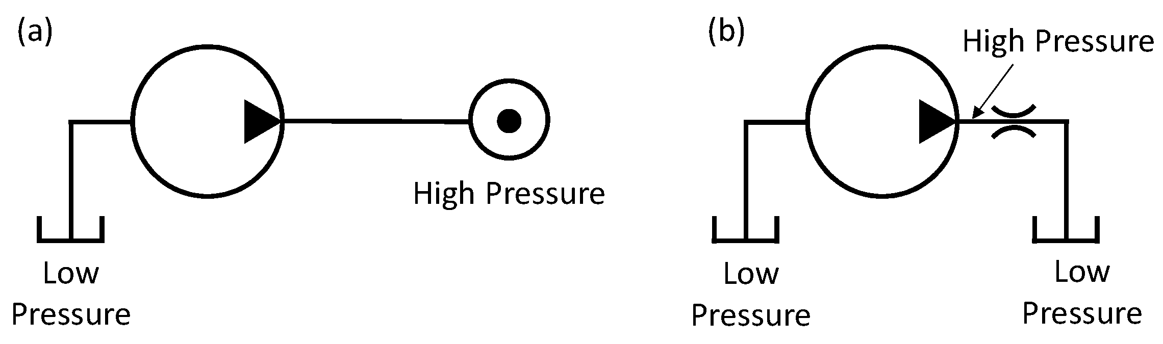
There are two idealized hydraulic circuits which are frequently taken as reference in pump testing and simulation: their conceptual schematic is shown in Figure 2. The first circuit is a volume-termination circuit (VT), which ideally connects the pump outlet directly to an infinitely large capacity at high pressure, which behaves as a high-pressure source. The second circuit is a restriction-termination circuit (RT), which uses a restriction to create the pressure loading at the pump outlet.
The same positive displacement pump provides delivery flow- and pressure-ripples which varies with the nature of the circuit: the VT circuit results in a small pressure ripple and a large flow ripple, while the RT circuit results in relatively large pressure ripple and negligible flow ripple (A small resistance effect, represented by the pump port restriction, is always present and might not be negligible. This small effect is also shown in Figure 3).
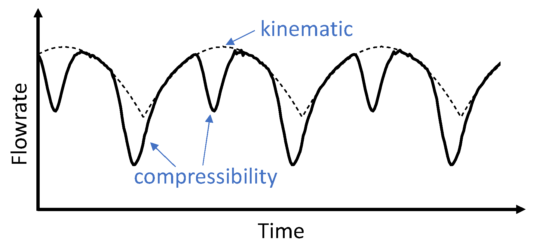
In this paper, the analysis of the outlet flow ripple of an EGP follows a two-step method. The first one being a separated analysis of the VT condition. In such conditions, the resistance from the circuit is zero, so that the flow ripple can be viewed as a flow source. The second step consists in the analysis of the influence of the load on the flow. Figure 4 shows a typical flow-ripple given by an EGP working under high pressure with the VT circuit. In the figure, the deviation from the kinematic ripple is caused by the backflows, which are the instantaneous flows from the delivery port that pressurize the internal displacement chambers (DCs) from the inlet pressure to the outlet pressure.
The above-mentioned pressurization component of the flow ripple for an EGP can be described with the help of Figure 5. When a tooth-space travels from the suction chamber and starts to get exposed to the high-pressure, the fluids contained in this tooth space is pressurized by an instantaneous flow rate that comes from the delivery port. The geometric location at which the DC pressurizes depends on the pump geometry and on the operating conditions, and it is a delicate aspect of the EGP design which is related to the radial balancing of the gears [18]. Figure 5 shows the case of the presence of backflow grooves connecting at the outer circumferential locations of the gears to the outlet port, which is common in several EGPs for high-pressure operation. This design usually implies a sudden exposure of the DC to the high-pressure ports. However, also with EGP designs where such groove is not present, the DC pressurization usually still occurs in a well concentrated region due to the non-uniformity of the sealing gap at the tooth tip of the gears. This non-uniformity results from the radial micro-motion of the gears under the pressure loading of the outlet [18]. In this case the starting point of the pressurization can be considered as the position where the tooth space starts to get exposed to large tooth-tip gaps. All these factors, in addition to other parameters of the EGP design affect the sharpness of the pressurization flow pulses qualitatively in shown in Figure 4. The sharper is the pressurization flow, the higher will be the deviation of the actual flow ripple with respect to the theoretical kinematic one.
While, the kinematic component of ripple source does not depend on the operating pressure of the EGP, it is clear that the magnitude of the ripple source given by the pressurization depends primarily on the pressure differential at the EGP ports. If this differential is minimum (close to zero), the influence of the pressurization ripple source vanishes. Instead, at high pressure condition the pressurization ripple source might become prominent compared to the kinematic ripple. This concept is depicted in Figure 6.
2.2. Simplified EGP Circuit
The most common lumped parameter approach to simulate flow through an EGP is to model the dynamic of its internal hydraulic circuit. In the past decade, a lot of models using this approach to simulate positive displacement pumps, such as [4,18,19,20], have been published and validated. This approach is also called lumped-element approach, in which each DC is modeled as a lumped element, and the physical quantities with each DC is assumed to be uniform, such as pressure, density, bulk modulus, etc. The fluid flow in between is represented by different models, such as turbulent orifices or laminar flows, depending on the geometry of the flow connection. For the reference pump, for a particular angular position of the gears, the hydraulic circuit to represent the fluid dynamics can be represented in Figure 7.
The fluid dynamics that describes the displacing action of an EGP (Figure 5) can be fully represented by the hydraulic circuit shown in Figure 7 (simplified as Figure 8 left), in which tooth spaces and the discharge chambers are modeled as displacement chambers with variable volumes, and the fluid flow between chambers are modeled as hydrodynamic flow connections. Obviously, the variable volume of each DC has to be considered to model the meshing region of the gears. In Figure 8 left, chambers with changing volumes are represented as equivalent piston-cylinder devices, with same laws for the volume variations. For EGPs with same number of teeth, the multiple DC system can be modelled as a sequence of pairs of DCs that always mesh together.
Based on the reasoning presented in Section 2.1, the flow ripple given by EGPs can be treated as the superposition of its fluid displacement component and pressurization ripple component.
The hydraulic circuits that represent each of these two components of ripple are shown in Figure 8 middle and right. The displacement circuit can be obtained by removing the pressure differential from the full EGP hydraulic circuit; the pressurization circuit can be obtained by disabling the volume changes (i.e., displacement chamber variations) from the full circuit.
The idea of superposition of solutions is based on the circuit with linear elements. Some hydraulic elements are non-linear; however, they can be linearized at specific operating condition under certain assumptions. For example, the displacement chamber volume can be written as linear capacitor assuming the bulk modulus of the oil is constant:
where capacitance given by a displacement chamber is written as
For orifice restrictors, the flow rate is written as:
which is not a linear relationship between pressure differential and resulting flowrate. However, by assuming the flowrate variation is small compared to the mean flowrate , the resistance of an orifice restrictor can be written as
With these linearized assumptions, the superposition can be applied. The superposition can be numerically validated by solving the flow ripple given by each of the two decoupled circuits shown in Figure 8 right and compared to the flow ripple solved from the full EGP circuit. Figure 9 qualitatively shows the overall flow ripple solution can be separated and superposing two decoupled solutions. It is necessary to clarify that in the displacement circuit shown in Figure 8, the low pressure in the delivery discharge chamber can be realized by setting the pressure of the outlet pressure source to be:
with the help of the linearized elements.
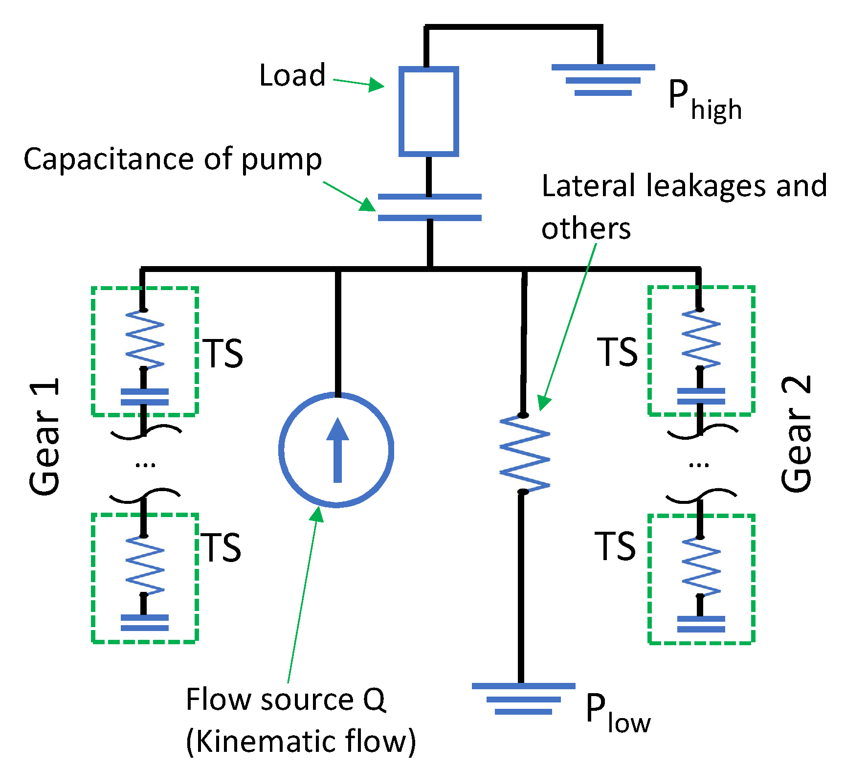
Based on their respective physics, the two decoupled circuits can be analyzed separately. The full circuit (Figure 7) can be further simplified into the circuit shown in Figure 10, in which the displacement source is in parallel with the pressurization source. For an EGP, the pressurization of the driver gear and driven gear occurs independently, therefore, the pressurization circuit of the driver gear and the one of the driven gear can be put in parallel. It has to be mentioned that the internal leakages (also shown in Figure 10), such as the leakages through the axial lubrication gaps at the gear’s lateral sides, will reduce the volumetric efficiency. However, they typically introduce little contribution to the ripple, since their effect on the instantaneous DC pressure is gradual and not localized as the tooth tip leakages that were examined in detail in the previous section. For this reason, this contribution is in this work neglected. As a consequence, in Figure 10 the lateral leakages are modeled as a single linear resistance in parallel to the ripple circuits.
It needs to clarify that, differently from the approaches discussed in past papers on the same topics [2,3,4,5,6,7,8,9], in which the capacitance and the impedance of a pump are discussed separately, this paper follows an approach where impedance effects associated with the displacement ripple source and the pressurization ripple source are evaluated separately. For each source, both capacitance and impedance (primarily resistance) effects are present. In the following sections, the analysis of the displacement solution and pressurization solution will be presented one after the other, with their respective sub-circuit representations.
3. Model of the Displacement Ripple Source
This section presents the analysis of the displacement ripple source mainly based on an analytical approach. For EGPs, the displacement ripple source is driven by the kinematic flow. The kinematic displacement given by a pair of gears has been discussed extensively in the past research [1,11,12,13,23,24]. However, due to the presence of contact points between the gears that involve trapped DCs, the fluid displacement will be achieved only when the position of relief groove is properly designed. A deviation from an optimum groove design results in an output kinematic flow that is different from the gear theoretical one. This section explains the flow coming out of displacement circuit (S1) in Figure 8, so that the relief groove positioning is a factor to be considered. The analysis of the influence of the relief groove positioning can be developed based on the volume curves that represent the fluid displacing action of a single DC, as it is explained in the rest of this section. For simplicity, the discussion of this section is based on EGPs with single-flank contact. Also, viscous effect, and the loading from the circuit will also influence the flow solution delivered by the displacement circuit, and they will be explained in this section as well.
3.1. Explanation Based on Volume Curves
The analysis based on the DC volume variation provides useful information about: (i) how to design the timing window of the relief groove for an EGP, and (ii) how the kinematic flowrate changes with the porting design.
The overall flow displacing action of an EGP can be studied observing the volume variation of a DC formed by one of more tooth spaces. The DC is first connected to the inlet port, and as the gear rotates it gets connected to the delivery and eventually back to the inlet region after passing through the meshing region. The meshing region determines the volume variation curve of the EGP. The reference arrangement of pump system and rotational direction was shown in Figure 1. On the volume curve, the zero angular position ( = 0) is defined to be the minimum volume position of the volume curve. As it moves to the left, the volume enters the coverage of delivery port; as it moves to the right at some point, the volume enters the coverage of suction port. Here three types of possible porting conditions are defined (Figure 11).
- (a)
- Connected porting: after getting out of the coverage of delivery port, the DC enters the suction port immediately, two porting coverages are connected.
- (b)
- Open-porting: there is a gap between the coverages of delivery and suction port, where the DC connects to neither delivery or suction port.
- (c)
- Overlapping porting: there is an angular interval of overlap: in this interval the DC is connected to both the delivery and the suction port.
Among these three porting designs, only the connected porting is the only meaningful porting condition for the kinematic analysis. In the open interval for the open-porting condition, the fluids in the DC will be fully trapped. With DC volume change, there will be a relevant pressure build up or cavitation which is likely to cause damages to the EGP. Eventually, as the gears rotate, the fluid will eventually go to the suction side. From the delivery flow standpoint, this case is equivalent to the connected-porting condition with a switching point at the end of the delivery window. Instead, the overlapping porting will result in a large bypass directly from high-pressure (outlet port) to low pressure (inlet port), which will result in large drop in the volumetric efficiency of the pump. In practice, a small overlapping-porting is often used to release internal DC pressure overshot. However, the kinematic analysis serves just as a macroscale description of the displacing action, and these small overlaps can be neglected and treated as connected porting condition. For this reason, in the rest of this paper, only the case of connected-porting design (Case A of Figure 11) is considered.
3.2. Analytical Expression of The Kinematic Flowrate Given by the Positioning of the Groove
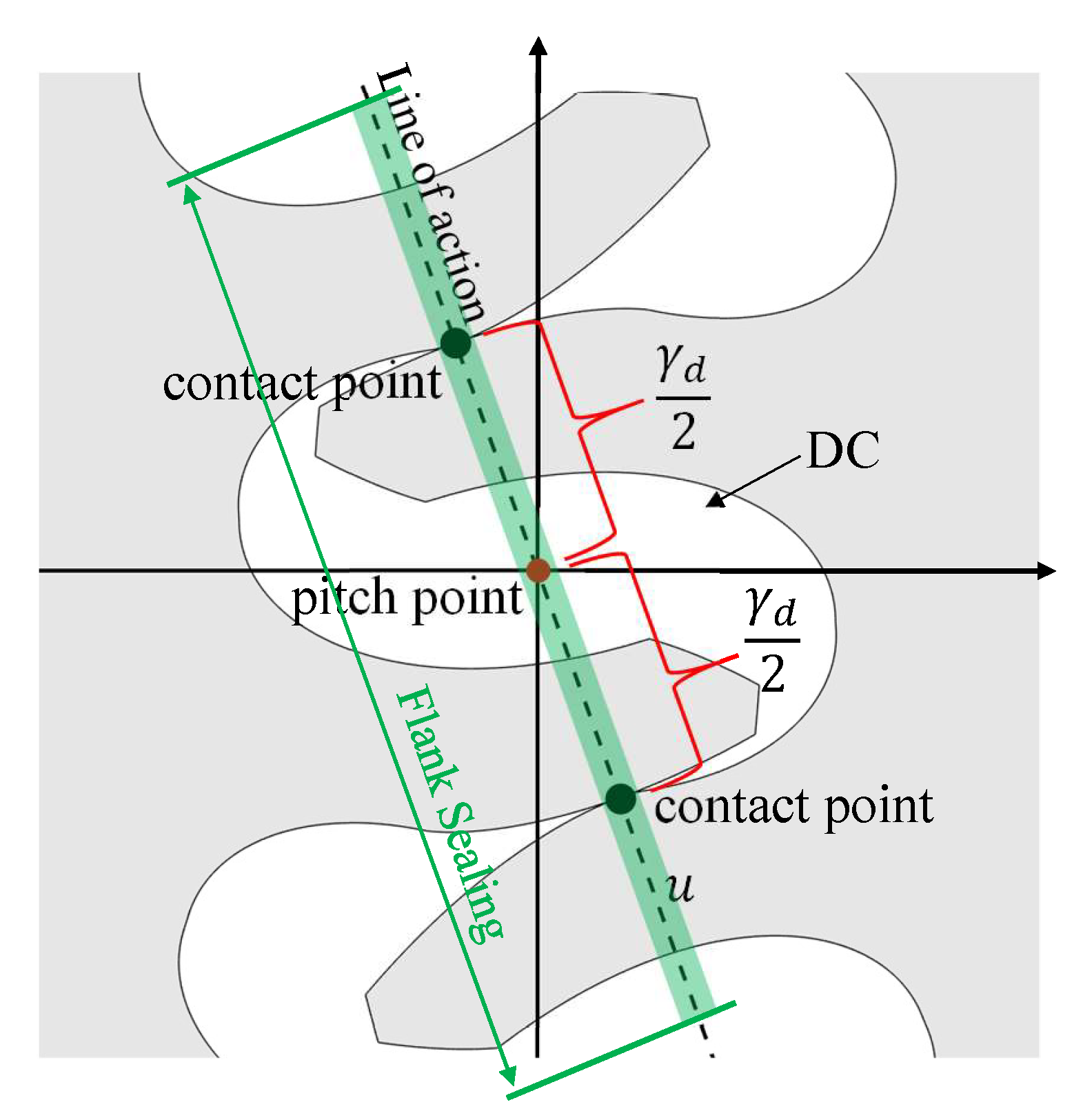
For common designs of EGPs, there is a geometric sealing region on the volume curve confined by the contact points of each gear. Out of this region, because of loss of tooth sealing, the DC will get exposed to the ports through a gap opening between teeth. Based on the convention of Figure 12, to the left and to the right of this region, the DC will get exposed to the delivery and the suction port, respectively. For single-flank EGP with profile contact ratio greater than one, this tooth-flank contact sealing region will be naturally formed, which belongs to the category of open porting condition defined in Section 3.1. Therefore, a single-flank EGP cannot operate purely relying on the radial flow connection, and relief grooves are required to establish the axial flow connection to connect two ports. The angular position at which the two windows connect will affect the kinematic flow and therefore the displacement ripple. In this paper, the angular positions at which the DC gets exposed to the delivery port and to the suction port between tooth flanks are defined as and , respectively.
For the derivation of kinematic flow, the lumped-parameter approximation was not considered, instead the classic analytical approach, which is based on conservation law first introduced by Bonacini [22], is used. The kinematic flowrate of external spur gear pump can be expressed as:
where H is the gear axial length, is the addendum radius of gears, i is the center distance between two gears. The only variable is u, which is distance between the delimiting contact point and the pitch point. This section will explain the definition of u at different gear-contact conditions and placement of grooves.
A more detailed geometry of a single-flank combined tooth-space is shown in Figure 13. Figure 13 also shows the position defined to be the zero-angle () position of the volume-curve, where the combined tooth-space (i.e., V1 + V2) reaches its minimum. Here Vi represents the volume of DCi illustrated in Figure 13. At this condition, the combined tooth-space is delimited by two contact points on the drive flank with equal distance to the pitch point.
The porting condition for involute EGP at the maximum delivery condition is shown in Figure 14 left, which means the combined displacement chamber switch from delivery port to suction port at its maximum volume position, which is the position. Assuming the gear pump is running at constant speed, the instantaneous position of the delimiting point u of an external spur gear pump at single-flank contact and maximum-delivery grooving settings can be written as:
where
defines the initial position. For the reference position define in Figure 13, . From now on, will be omitted by assuming it is zero without further specification. As both delimiting contact points of the combined tooth-space is on the primary line of action, the tooth-flank sealing is defined by the contact ratio on the primary line of action . The length of the tooth-flank sealed region on the primary line of action is , with its center point located at the pitch point. is the base pitch for the drive flank
Considering the condition without any relief groove, the tooth-flank sealing interval (see Figure 12) is:
and the position of and can be located as
For involute gear pumps to drive itself, its primary contact ratio should be greater than 1, i.e.,
Therefore, there will be , which means that without relief groove there will be open-porting condition, and indicates that the design of relief groove is necessary for this type of EGP.
The groove position with minimum delivery will be the connected-porting design with port-switching angle at either or (shown in Figure 14). Because of symmetry, these two options will have the same effect on kinematic mean flowrate or flow non-uniformity, with difference only in a flipped ripple shape for each cycle. For the porting design that port-switching angle is at , the resulting active delimiting point position can be written as:
where
The comparison between the groove geometry for maximum-delivery and minimum-delivery is shown in Figure 15. To achieve the same porting on the volume-curve, there are an infinite number of possible designs, Figure 15 just shows two examples with the simplest rectangular groove designs.
If the volume-curve porting is made such that the port-switching angle is between the maximum-delivery and the minimum-delivery, the kinematic mean flowrate and flow non-uniformity will also fall in between these two conditions. A parameter ‘relief groove coefficient’ is defined to quantify the porting condition given by a groove design: when , it is the maximum-delivery relief groove design; when , it gives the minimum-delivery groove design.
At an intermediate porting condition with , the active delimiting point position can be written as:
where
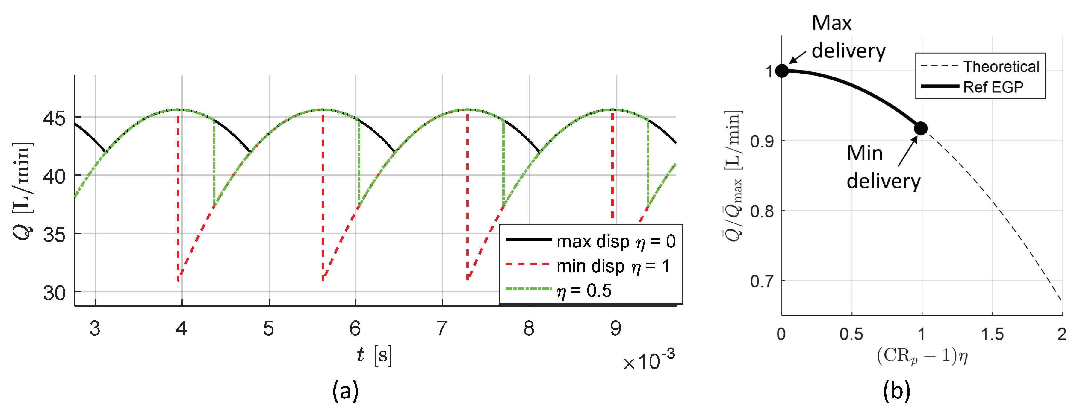
The kinematic flow ripple given by the same pair of gears but different groove positionings are shown and compared in Figure 16a. Three different grooves compared are (maximum delivery), (minimum delivery) and . The mean flowrate can be integrated as
Figure 16b shows the drop of mean flowrate for a reference pump with respect to the change of .
3.3. Viscous Effects
The fluid-dynamic effects (such as viscous effect) can be considered as an additive effect to the kinematic flow. As a consequence, being the displacement ripple solution defined as the output from the circuit shown in Figure 8 (middle schematic, S1), the fluid-dynamic effect is also part of the displacement solution.
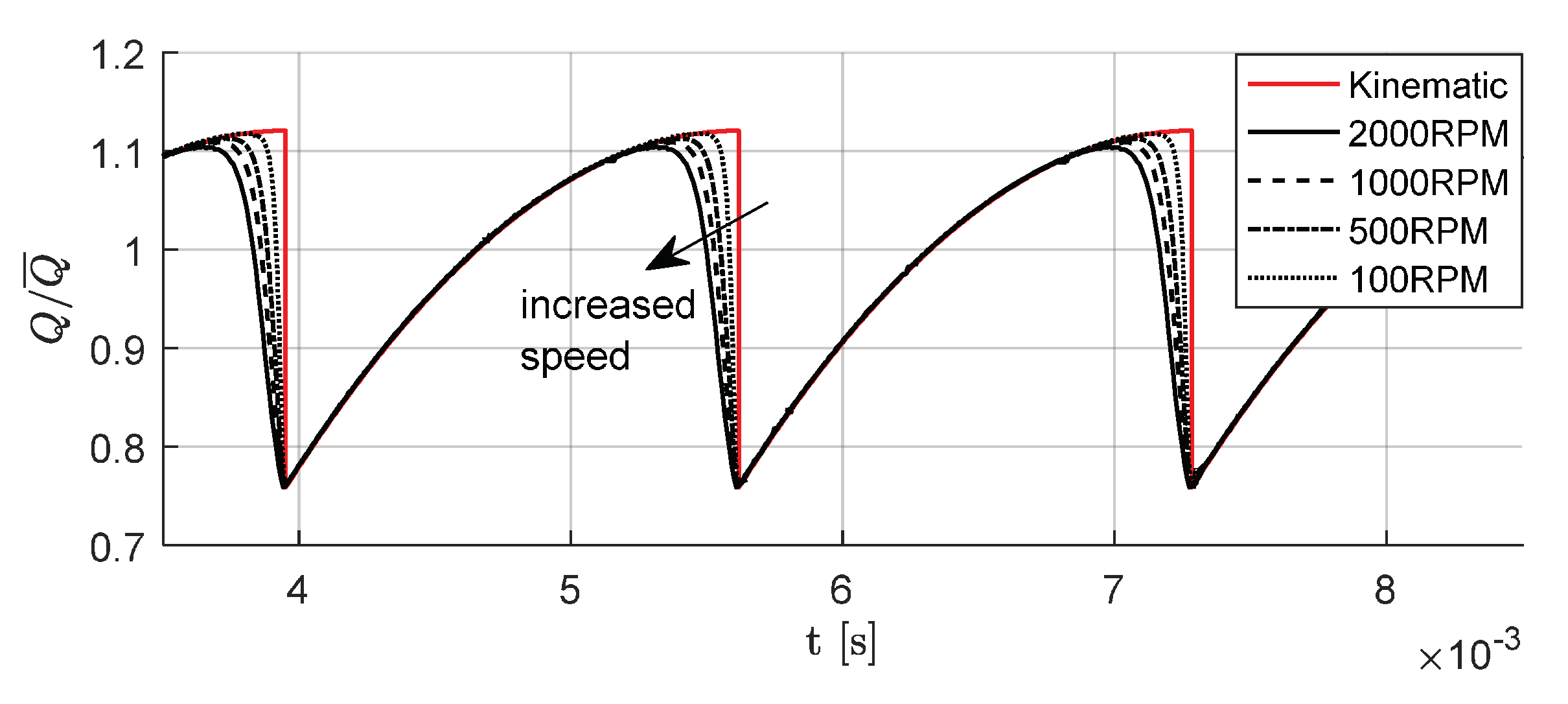
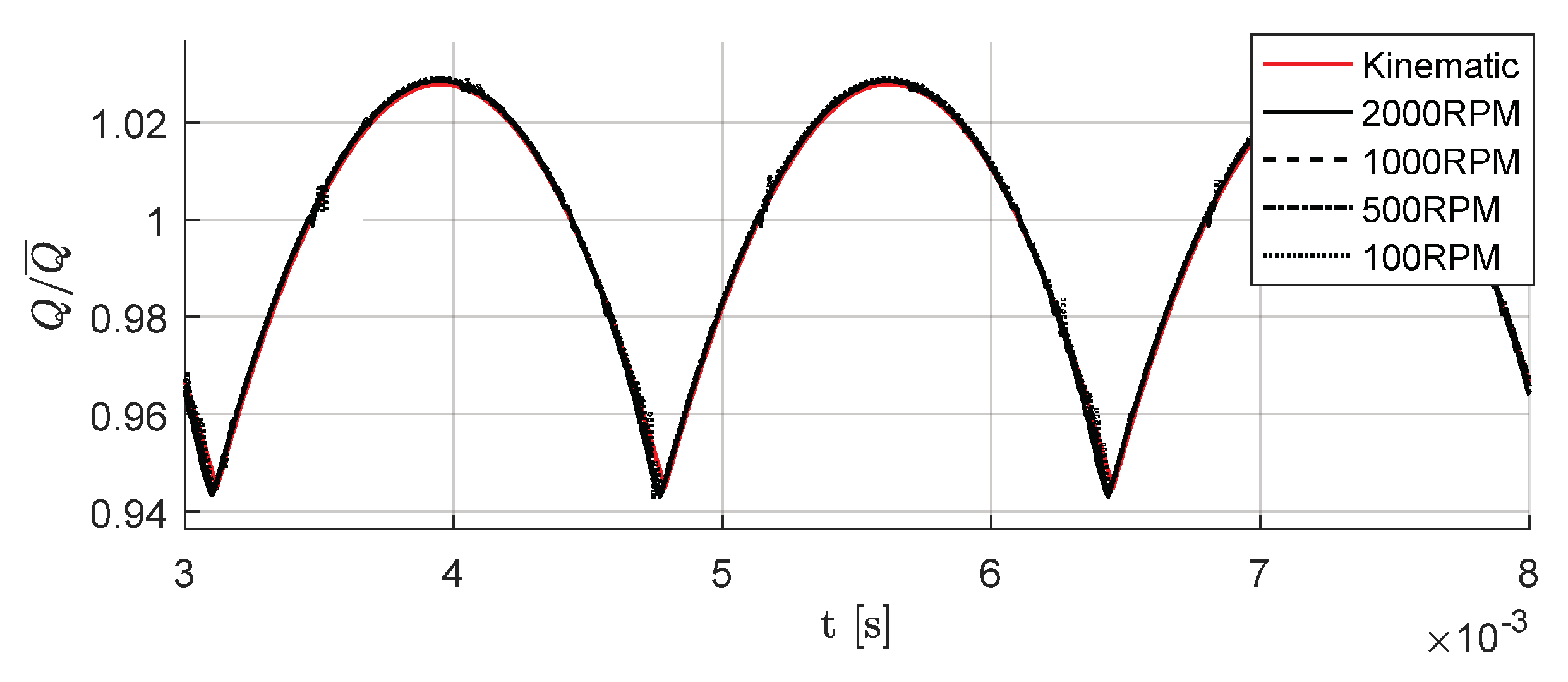
The difference between the fluid-dynamic flow ripple and the kinematic flow ripple is given primarily by the viscosity effects. Moreover, the port configuration will also influence the difference between kinematic and fluid-dynamic flow ripple. Figure 17 and Figure 18 show the fluid-dynamic ripple for the reference pump at minimum and maximum delivery porting condition, respectively. These results are simulated with the VT circuit using a zero pressure differential, with a large variation of shaft speed, from 100 RPM to 2000 RPM. This is the condition where the loading is infinitely small, and the fluid-dynamic flow at outlet al.most recovers to its kinematic ripple at the maximum-delivery porting condition (Figure 18). The flow pattern is consistent almost regardless of the changes in shaft speed. However, for the minimum-delivery porting condition, the speed-dependent effects appear, and the discrepancy gets larger as the speed is increased. A similar effect can be observed for variations of the fluid viscosity: higher viscosity will lead to larger discrepancy at non-maximum-delivery porting condition. This effect can be explained as follows: if the groove porting switches from the outlet to inlet during a DC volume change (either a compression or expansion), at the switching point the opening connection is so small that the viscous effect will stop the fluids from being pumped out or sucked in. The results in Figure 17 and Figure 18 further indicate that with zero pressure differential, dynamic flow and kinematic flow can still be different, which is given by different fluid-dynamic effects.
3.4. Effect of the Delivery Circuit
As pertains to the delivery circuit, this paper considers the simplistic case in which the pump load consists of a capacitance and a resistor, so that the inductance of the delivery line is neglected. This case is representative of situations where the pump operates with short delivery lines, compared to the speed of sound, so that wave propagation effects are negligible. For the kinematic solution (S1), the stand-along hydraulic circuit connection is shown in Figure 19, which simply connects the kinematic flow source in series with the pump capacitance C and a loading resistance R. It is worth mentioning that the volume used for defining the pump capacitance represents all the volumes of both the delivery discharge groove and the backflow groove. More details about the assumptions related to the backflow grooves are discussed in the next Section 4.
Based on the linearized capacitance and resistance model from Equation (1) to Equation (4) for displacement chamber and orifice, the differential equation for this simple circuit can be written as:
By solving this equation, the outlet flow ripple can be solved as:
where
Next, the influence given by the loading on the flow source can be determined. For the flow sources, the transfer function can be determined as the ratio of the flow without loading (i.e., the flow source itself) to the flow under loading. For the simple circuit considered here, the loading to the flow source is a pump capacitance and a resistance given by the restrictor.
The influence of the circuit can be measured as a transfer function h, which is defined as the ratio between the flow ripple with no load (i.e., ) and that under load (), i.e.,
By definition , therefore, the transfer function of the restrictor in the RT circuit can be written as
In this case, it can be re-written as
The transfer function given by the load is
The analytical results of the kinematic ripple source presented in this section (by substituting Equations (7), (13) and (15) into Equation (6)) can be written in the form of Fourier Cosine Series. After that, the transfer function of Equation (25) can be super-imposed to yield the resulting delivery flow ripple under different loading level. Figure 20 shows the change of the kinematic ripple under different loading condition by comparing the kinematic solution for the VT circuit and the RT circuit of Figure 2.
4. Model of the Pressurization Ripple
The hydraulic circuit representation of the pressurization ripple source was shown by the circuit S2 in Figure 8. This circuit can be further simplified on the basis of some physical considerations. The pressurization of the DCs in a EGP happens only at the outer circumference, where each DC carries the from the suction chamber to the delivery environments. During this path, the fluid volume inside the DC is pressurized (Figure 5). The phenomena that occur in the meshing zone contributes mainly to the kinematic part of the delivery flow ripple and they can be isolated from the pressurization ripple source. This is a spatial separation which makes the analysis of the pressurization ripple independent from the analysis of the displacement solution.
Under the assumption explained above, the analysis of the pressurization ripple source can be made with the simplified circuit shown in Figure 21, where the DCs are in series to be pressurized. Each DC is modeled by a linear capacitor for modeling the pressure build-up in each tooth space, together with a linear resistance for modeling the fluid flow connection between adjacent tooth spaces. It is necessary to clarify that, the pressurization ripple source discussed in this paper, is a source term that generates a net flowrate over time. Although it is essentially driven by the capacitance of pump DCs, it has to be considered as a source instead of a capacitive element in a hydraulic circuit, as considered in most of the past papers.
4.1. Single-DC Pressurization Problem
First, the simple case of the pressurization of an EGP without backflow grooves and a perfect DC sealing (zero tooth tip leakage and lateral leakage) is considered. In this case, the tooth space volumes are pressurized when they reach the delivery chamber one by one. When one is being pressurized, the rest of tooth spaces remain unaffected. Therefore, for the representation of Figure 21, only one tooth space instead of a series of tooth spaces is included. The kinematics considered in this problem and the corresponding hydraulic circuit is shown in Figure 22. For this single-DC pressurization linearized system, the differential equation is written as:
where
Thus, the linear system for a characteristic solution can be normalized as
with initial condition
where , , , , are the normalized parameters given by:
The normalized time constants of this linear system are:
The time constant represents a solution that depressurizes the DCs. The time scale of the single-DC pressurization solution is determined by . For the volume-termination circuit, , while for the restrictor-termination circuit, . As the total amount of the pressurization fluids, i.e., the integral of the pressurization flow for the DCs, is the same, the magnitude of the pressurization ripple is scaled with time constant:
The influence of the change of and on the solution as well as an illustration of the time constants are shown in Figure 23, where is the mean flow required to pressurize a single tooth space:
where n is the shaft speed, V is the volume of tooth space, K is the bulk modulus, and is the working pressure difference between the outlet port and the inlet port.
The resulting flow ripple given by the single-DC pressurization is . Therefore, the flow ripple given by the pressurization of one gear is:
The total pressurization ripple is given by the combined effect of the two gears of the EGP. Because of the meshing of two gears, there is a phase delay in the gear profile angle, therefore:
where . For the reference gear pump at the particular gear center distance 33.36 mm, the phase delay between two gears is , which involves geometric calculation according to the gear pump design.
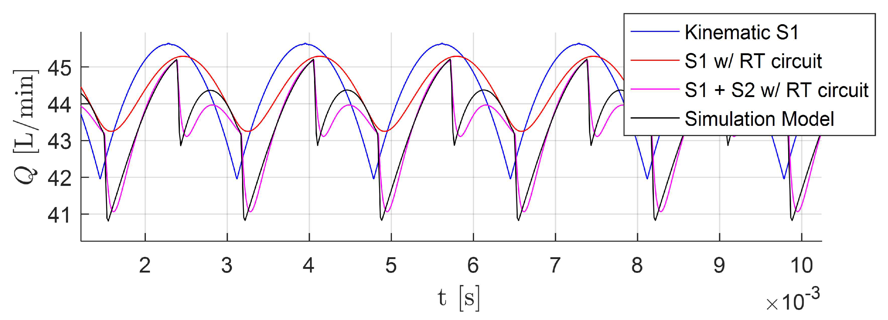
The recovery of the flow ripple is simulated by superposing the analytical kinematic solution and the pressurization solution from the linearized analysis presented in this section. For the single-DC pressurization problem with the reference gear pump at a restriction-termination circuit, at 2000 RPM and 200 bar operating condition, the comparison to the flow ripple from the simulation model [18] is shown in Figure 24. It is shown that the superposition of the S1 and S2 solutions based on the analysis above successfully reproduced the flow ripple from the simulation model under the RT circuit.
Although the single-DC pressurization problem discussed above is for a simplified configuration, the single-DC pressurization approach can be generalized to a more realistic configuration: the overall pressurization solution can always be regarded as the superposition of repeating single-DC pressurization solution. For linearized considerations, for any realistic condition (Figure 21), a linearized effective resistance (R1 in the circuit in Figure 22) can be used as a replacement to all the hydraulic elements in Figure 21 between the first DC and the circuit load, to quantify the smoothness of the pressurization for each DC.
4.2. Results of Pressurization Ripple Solution
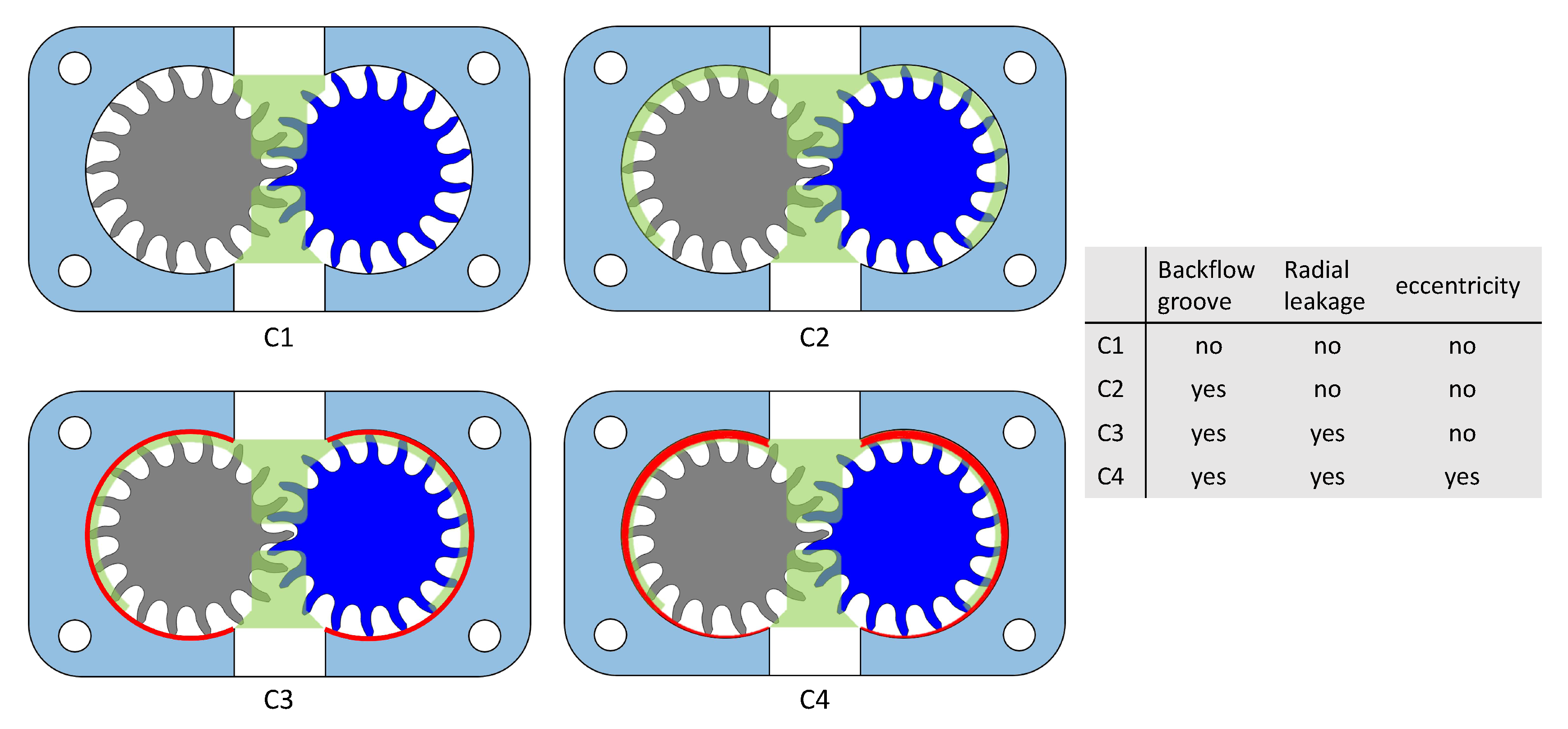
From the considerations made in the previous sections, the pressurization solution can be analyzed separately. This section presents the pressurization solution (S2) produced by the reference pump under VT and RT circuit connections. All the results are produced by the lumped-parameter simulation model [18], simulated under the operating condition of 2000 RPM and 200 bar. For each circuit, four different configurations are considered: the first configuration C1 does not have backflow groove, and is assumed to have perfect radial tooth-tip sealing, which is the same as the single-DC pressurization problem presented in Section 4.1. The second configuration C2 adds the backflow groove to C1, with perfect radial sealing still assumed; instead, C3 adds a uniform 0.015 mm tooth-tip gap to C2, where the gear is concentric to the casing. Finally, C4 uses the same nominal radial clearance as C3, while the gear is eccentric towards the suction by 0.015 mm. These four testing conditions are also illustrated in Figure 25.
The pressurization solutions for VT and RT circuits are shown in Figure 26 and Figure 27, respectively. For each circuit, C1 gives the steepest pressurization, and also the largest flow ripples. In this case, the pressurization flow goes only though the radial passage between a gear tooth and the edge of the casing. In general, the radial passage opens suddenly as the gear tooth moves out of the casing at high speed. In C2, the DCs are pressurized via the small passage on the lateral sides in the backflow groove, therefore the pressurization is smoother. In C3, the uniform distribution of tooth tip gap creates a high leakage under 200 bar high-pressure operating condition. However, this circumferential leakage further smoothens the pressurization solution. The configuration C4, which is more representative of the actual EGP operation under high pressure (because it considers the eccentric gear position), the radial gap on the suction side approaches zero, preventing high tooth tip leakages to the suction. However, the eccentric position of the gears also creates a rapid increase of the tooth tip gap after its minimum position, creating a steep pressurization effect on the DC. From one side, this eccentric position creates a high volumetric efficiency, but on the other hand it results with a higher delivery flow ripple. This results in a close comparison between C2 and C4, the existence of a radial gap increases the connection area for the region covered by the backflow groove, and it provides a small opening reaching out of the coverage of backflow groove. This makes an earlier the pressurization of the DC fluids. However, the overall effect compared to C2 based on the simulation result is quite small.
The frequency analysis of the same flow ripples better highlights these trends. For the steep pressurization in C1, high frequency components for almost all harmonics can be observed; while for other cases, only the first few harmonics are prominent. The trend is consistent for both the VT and the RT circuits, only the magnitude of each harmonic is smaller for the RT circuit.
4.3. Numerical Analysis for the Transfer Function of the Circuit
It is clear that the displacement ripple solution can be viewed as a flow source, as it is driven by the kinematic flow source, as explained in Section 3. However, based on the analysis in Section 4.1, the behavior of the pressurization solution S2 is substantially different from a flow source. Therefore, it cannot be assumed that the transfer function given by the circuit load to S2 is the same as the kinematic solution S1 without further verification. This section presents a study on the transfer function of the circuit load in a numerical way, as the nature of the pressurization source is non-linear, and an analytical solution is not easy to derive. This is made with the simple circuit that has the pump connected to a single restrictor before a pressure source with short pipe (pressurization solution S2). The transfer function is defined the same way as for the displacement ripple solution S1, that is the ratio between the outcoming flowrates from VT circuit and RT circuit, Equation (23).
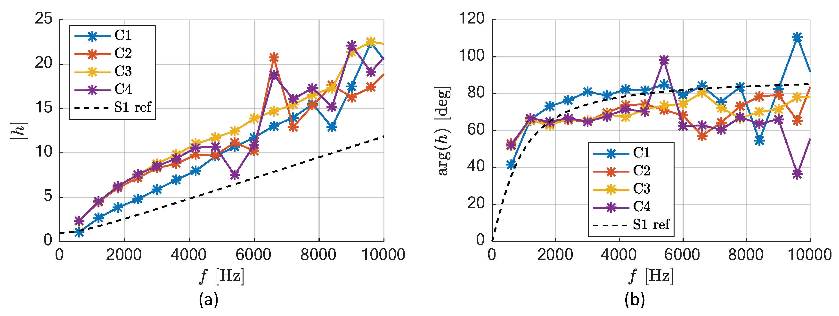
The transfer function for the S2 solution for the VT and RT circuits can shown in Figure 28 and Figure 29, for two different pressure conditions (respectively 100 bar and 200 bar). The transfer function is calculated for all four configurations (from C1 to C4), and it is shown that the effect from the circuit are consistent for both selected operating conditions.
Compared to the transfer function for the kinematic solution (the dashed line in Figure 28 and Figure 29), the result shows that at 200 bar, the phase delay is similar, while the magnitude of the transfer function h is about twice for S2 than for S1. This means that as the resistance in the circuit increases, the reduction of the magnitude of S2 solution is about twice of that for the kinematic solution S1. However, when the same pump is working at the reduced pressure (100 bar condition), the magnitude of the transfer function is similar for S1 and S2, and phase delay is slightly smaller than that at 200 bar condition. It can be shown that the transfer function for the pressurization ripple is strongly pressure-dependent. On the other hand, the displacement ripple is independent to the pressure condition. Although this numerical study is exploratory and made for simple circuit connection, it shows that two sources of the pump ripple react to the load of the hydraulic circuit very differently.
The result presented above indicates that the pressurization ripple source cannot be merged with the displacement ripple source, as a single flow source in the circuit. This because the two components have quite different physical behavior, and therefore they should be modeled in a different way. At least for an external gear pump, this is in contrast with what can be deducted from the general literature that suggests modeling the pump as a flow source with an impedance.
5. Conclusions
This paper presented a theoretical analysis for the source of the delivery flow pulsations for external gear pumps. First, the linearization approach for the fluid dynamics of an EGP is described, providing the basis for separation of analysis and superposition of two ripple sources. The following two sections give the analysis and the derivation of the characteristic solutions for two ripple sources, namely, the displacement source and the pressurization source.
The main discovery of this paper can be summarized in the following. The ripple produced by an external gear pump can be considered as the superposition of two ripple solutions: the displacement solution, and the pressurization solution. The displacement solution is given by the volume change of the displacement chambers, which happens in the meshing zone. The displacement solution takes the kinematic flow of the gears as input, and evaluate an actual delivery flow considering the position of the relief (or timing) grooves, the viscosity of the fluid and the features of the delivery system used as pump load. On the other hand, the pressurization solution is given by the pressure differential, and it develops at the outer circumference of gear rotation. The overall pressurization solution can be analyzed by the superposition of the single-DC pressurization solution.
Under the assumption of linearized hydraulic elements (DCs as linear capacitors and restrictors as linear resistors), the response of both solutions to the load in the hydraulic circuit can be studied analytically or numerically. For the displacement solution, the circuit is driven by a flow source, which is the kinematic flow given by the gear rotation modified by the position of the relief groove. With the geometric analysis based on the volume curve presented in Section 3 of the paper, the flow source term is derived analytically for single-flank spur gear pumps. The same can be done for other types of gear pumps, such as dual-flank gear pumps, or helical gear pumps, with slight modification of the presented procedure. A Fourier analysis of the source term is performed to obtain the influences on different frequency content of the solution, given by the change of a circuit load. For the pressurization solution, firstly a characteristic solution for a single DC pressurization problem is derived to represent the physics for the source of pressurization ripple. This single-DC pressurization problem can be viewed as a linearization of the pressurization of a DC in an actual gear pump. In this way, two time constants can be used for characterizing the sharpness of the pressurization pulsation. The frequency response to the circuit loading and the resulting transfer function can be obtained numerically by taking the ratio between the solutions from restriction-terminated circuit and the volume-terminated circuit.
The results presented in the paper illustrate an exploratory study for a simple hydraulic circuit where the EGP pressure loading is represented by a restriction. The result shows that the restriction in the circuit causes different transfer-function effects (relation between the source flow and the actual flow ripple) for two ripple sources. For example, at 2000 RPM and 200 bar condition, it is found that the transfer function given by the restriction gives about twice in magnitude to the pressurization solution than to the kinematic solution. This result indicates that an EGP cannot be assumed as a single flow source, as the two components of its ripple source have very different behaviors in a circuit with respect to circuit loadings. This indication is against the method that has been traditionally used by many researchers, such as “secondary-source” method. Especially for high-pressure application, where the pressurization ripple source is strong, the error can be large. Based on the analysis presented in this paper, potentially a new experimental method can be formulated, to determine the kinematic source and the pressurization source separately: kinematic source can be obtained from analyzing the gear geometry and the groove position, while the pressurization source can be determined by experimentally determining the linearized resistance for the single-DC pressurization problem.
Author Contributions
Conceptualization, X.Z. and A.V.; methodology, X.Z. and A.V.; validation, X.Z.; formal analysis, X.Z.; investigation, X.Z.; writing—original draft preparation, X.Z.; writing—review and editing, X.Z. and A.V.; visualization, X.Z.; supervision, A.V.
Funding
This research received no external funding.
Conflicts of Interest
The authors declare no conflicts of interest.
Nomenclature
| Latin Symbols | |
| A | area (m) |
| C | capacitance (m/Pa) |
| discharge coefficient | |
| CR | contact ratio |
| f | frequency (Hz) |
| h | transfer function |
| H | axial length of a gear (mm) |
| i | center distance (mm) |
| K | bulk modulus (bar) |
| m | module of a gear (mm) |
| M | arbitrary integer |
| N | number of teeth |
| p | pressure (bar) |
| initial pressure (bar) | |
| Q | flowrate (L/min) |
| mean flowrate (L/min) | |
| R | resistance (Pa/m-s) |
| addendum radius (mm) | |
| t | time (s) |
| initial time (s) | |
| T | constant to define a time interval (s) |
| u | position of the contact point on the line of action (mm) |
| V | volume (m) |
| Greek Symbols | |
| Tool pressure angle of a gear (degree) | |
| Base pitch of a gear (mm) | |
| Magnitude of the flow ripple (L/min) | |
| Relief groove coefficient | |
| Density (kg/m) | |
| Time constant (s) | |
| Angular position (degree) | |
| Phase shift (degree) | |
| Angular velocity (degree/s) | |
| Subscript | |
| a | Addendum |
| crit | Critical |
| d | Driver gear |
| del | Delivery |
| k | Kinematic |
| p | Profile (profile contact ratio) |
| S1 | Displacement ripple solution |
| S2 | Pressurization ripple solution |
| suc | Suction |
Abbreviations
| DC | Displacement chamber |
| EGP | External gear pump |
| RT | Restriction-termination |
| VT | Volume-termination |
References
- Ivantysyn, J.; Ivantysynova, M. Hydrostatic Pumps and Motors; Akademia Books International: New Delhi, India, 2001. [Google Scholar]
- Edge, K.; Johnston, D. The “secondary source” method for the measurement of pump pressure ripple characteristics Part 1: Description of method. Proc. Inst. Mech. Eng. Part A J. Power Energy 1990, 204, 33–40. [Google Scholar] [CrossRef]
- Edge, K. “Secondary source” method for the measurement of pump pressure ripple characteristics Part 2: Experimental results. Proc. Inst. Mech. Eng. Part A J. Power Energy 1990, 204, 41–46. [Google Scholar] [CrossRef]
- Kojima, E.; Yu, J.; Ichiyanagi, T. Experimental determining and theoretical predicting of source flow ripple generated by fluid power piston pumps. SAE Trans. 2000, 109, 348–357. [Google Scholar]
- O’Neal, D.; Maroney, G. Measuring pump fluid-borne noise generation potential. BFPR J. 1978, 11, 235–241. [Google Scholar]
- Kojima, E.; Shinada, M. Characteristics of fluidborne noise generated by fluid power pump: 3rd report, discharge pressure pulsation of external gear pump. Bull. JSME 1984, 27, 2188–2195. [Google Scholar] [CrossRef]
- Edge, K.; Wing, T. The measurement of the fluid borne pressure ripple characteristics of hydraulic components. Proc. Ins. Mech. Eng. Part B Manag. Eng. Manuf. 1983, 197, 247–254. [Google Scholar] [CrossRef]
- Nakagawa, S.; Ichiyanagi, T.; Nishiumi, T. A consideration on the behavior of hydraulic pressure ripples in relation to hydraulic oil temperature. In ASME/BATH 2015 Symposium on Fluid Power and Motion Control; American Society of Mechanical Engineers: New York, NY, USA, 2015. [Google Scholar]
- Nakagawa, S.; Ichiyanagi, T.; Nishiumi, T. Experimental investigation on effective bulk modulus and effective volume in an external gear pump. In BATH/ASME 2016 Symposium on Fluid Power and Motion Control; American Society of Mechanical Engineers: New York, NY, USA, 2016. [Google Scholar]
- Hydraulic Fluid Power—Determination of Pressure Ripple Levels Generated in Systems and Components— Part 1: Method for Determining Source Flow Ripple and Source Impedance of Pumps; International Standard ISO 10767-1; ISO: Geneva, Switzerland, 2015.
- Manring, N.D.; Kasaragadda, S.B. The theoretical flow ripple of an external gear pump. J. Dyn. Syst. Meas. Control Trans. Asme 2003, 125, 396–404. [Google Scholar] [CrossRef]
- Zhao, X.R.; Vacca, A. Numerical analysis of theoretical flow in external gear machines. Mech. Mach. Theory 2017, 108, 41–56. [Google Scholar] [CrossRef]
- Zhao, X.; Vacca, A. Formulation and optimization of involute spur gear in external gear pump. Mech. Mach. Theory 2017, 117, 114–132. [Google Scholar] [CrossRef]
- Yoon, Y.; Park, B.H.; Shim, J.; Han, Y.O.; Hong, B.J.; Yun, S.H. Numerical simulation of three-dimensional external gear pump using immersed solid method. Appl. Therm. Eng. 2017, 118, 539–550. [Google Scholar] [CrossRef]
- Qi, F.; Dhar, S.; Nichani, V.H.; Srinivasan, C.; Wang, D.M.; Yang, L.; Bing, Z.; Yang, J.J. A CFD study of an electronic hydraulic power steering helical external gear pump: Model development, validation and application. SAE Int. J. Passen. Car Mech. Syst. 2016, 9, 346–352. [Google Scholar] [CrossRef]
- Castilla, R.; Gamez-Montero, P.J.; Ertürk, N.; Vernet, A.; Coussirat, M.; Codina, E. Numerical simulation of turbulent flow in the suction chamber of a gearpump using deforming mesh and mesh replacement. Int. J. Mech. Sci. 2010, 52, 1334–1342. [Google Scholar] [CrossRef]
- Castilla, R.; Gamez-Montero, P.J.; Del Campo, D.; Raush, G.; Garcia-Vilchez, M.; Codina, E. Three-dimensional numerical simulation of an external gear pump with decompression slot and meshing contact point. J. Fluid Eng. 2015, 137, 041105. [Google Scholar] [CrossRef]
- Vacca, A.; Guidetti, M. Modelling and experimental validation of external spur gear machines for fluid power applications. Simul. Modelling Pract. Theory 2011, 19, 2007–2031. [Google Scholar] [CrossRef]
- Mucchi, E.; Dalpiaz, G.; del Rincon, A.F. Elastodynamic analysis of a gear pump. Part I: Pressure distribution and gear eccentricity. Mech. Syst. Signal Process. 2010, 24, 2160–2179. [Google Scholar] [CrossRef]
- Zhao, X.; Vacca, A. Analysis of continuous-contact helical gear pumps through numerical modeling and experimental validation. Mech. Syst. Signal Process. 2018, 109, 352–378. [Google Scholar] [CrossRef]
- Mucchi, E.; D’Elia, G.; Dalpiaz, G. Simulation of the running in process in external gear pumps and experimental verification. Meccanica 2012, 47, 621–637. [Google Scholar] [CrossRef]
- Battarra, M.; Mucchi, E. A method for variable pressure load estimation in spur and helical gear pumps. Mech. Syst. Signal Process. 2016, 76, 265–282. [Google Scholar] [CrossRef]
- Bonacini, C. Sulla Portata delle Pompe ad Ingranaggi; L’Ingegnere: Milan, Italy, 1961. (In Italian) [Google Scholar]
- Kasaragadda, S.D.; Manring, N.D. The theoretical flow ripple of an external gear pump. In ASME 2002 International Mechanical Engineering Congress and Exposition; American Society of Mechanical Engineers: New York, NY, USA, 2002. [Google Scholar]
Figure 1.
Cross sectional view of an EGP. The tooth space volumes are colored according to their pressure during a typical operation.
Figure 1.
Cross sectional view of an EGP. The tooth space volumes are colored according to their pressure during a typical operation.

Figure 2.
Two different methods of analysis of the pump outlet flow fluctuations: (a) volume-termination (VT) (b) restriction-termination (RT).
Figure 2.
Two different methods of analysis of the pump outlet flow fluctuations: (a) volume-termination (VT) (b) restriction-termination (RT).

Figure 3.
Comparison of (a) the flow ripple and (b) the pressure ripple for the reference pump working at 2000 RPM, 200 bar operating condition at VT and RT circuits.
Figure 3.
Comparison of (a) the flow ripple and (b) the pressure ripple for the reference pump working at 2000 RPM, 200 bar operating condition at VT and RT circuits.

Figure 4.
Two major components of the ripple sources: compressibility, and the kinematic flow (dashed line). Produced with the reference pump at 2000 RPM, 200 bar operating condition and VT circuit.
Figure 4.
Two major components of the ripple sources: compressibility, and the kinematic flow (dashed line). Produced with the reference pump at 2000 RPM, 200 bar operating condition and VT circuit.

Figure 5.
A gear pump with a tooth-space being pressurized by the backflow groove.

Figure 6.
Flow-ripple compared to the kinematic flow at 200 bar and 20 bar (simulated based on the reference EGP with 2000 RPM and VT circuit).
Figure 6.
Flow-ripple compared to the kinematic flow at 200 bar and 20 bar (simulated based on the reference EGP with 2000 RPM and VT circuit).

Figure 7.
The hydraulic circuit used in the HYGESim simulation tool for modeling the displacing action of and EGP. The representation for the hydraulic circuit of an EGP is similar to [22].
Figure 7.
The hydraulic circuit used in the HYGESim simulation tool for modeling the displacing action of and EGP. The representation for the hydraulic circuit of an EGP is similar to [22].

Figure 8.
The overall lumped-parameter model circuit and two decoupled circuits. The decoupled circuits can reproduce the displacement solution (S1) and the pressurization solution (S2) respectively.
Figure 8.
The overall lumped-parameter model circuit and two decoupled circuits. The decoupled circuits can reproduce the displacement solution (S1) and the pressurization solution (S2) respectively.
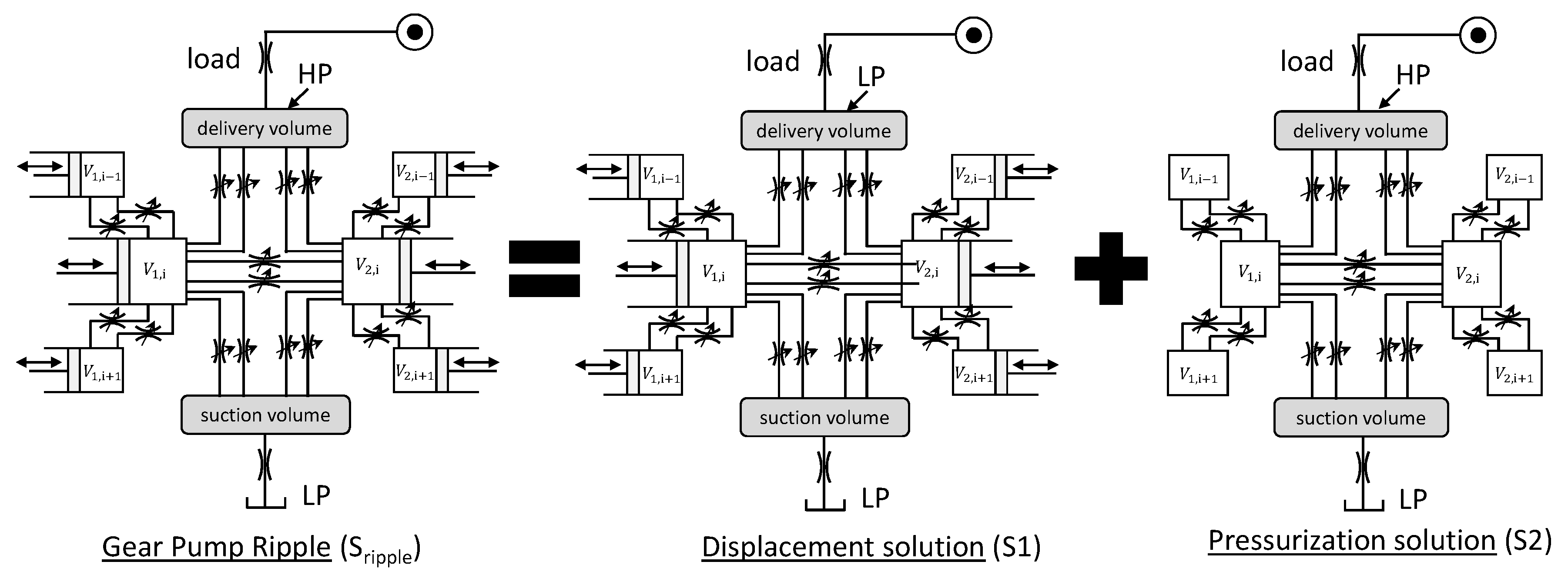
Figure 9.
Solution of the decoupled solution and their superposition.

Figure 10.
Simplified circuit representing the flow delivery of an EGP.

Figure 11.
Three porting conditions based on volume curve: (a) connected porting (b) open porting (c) overlapping porting.
Figure 11.
Three porting conditions based on volume curve: (a) connected porting (b) open porting (c) overlapping porting.

Figure 12.
Tooth-flank contact sealing for EGPs without relief groove.
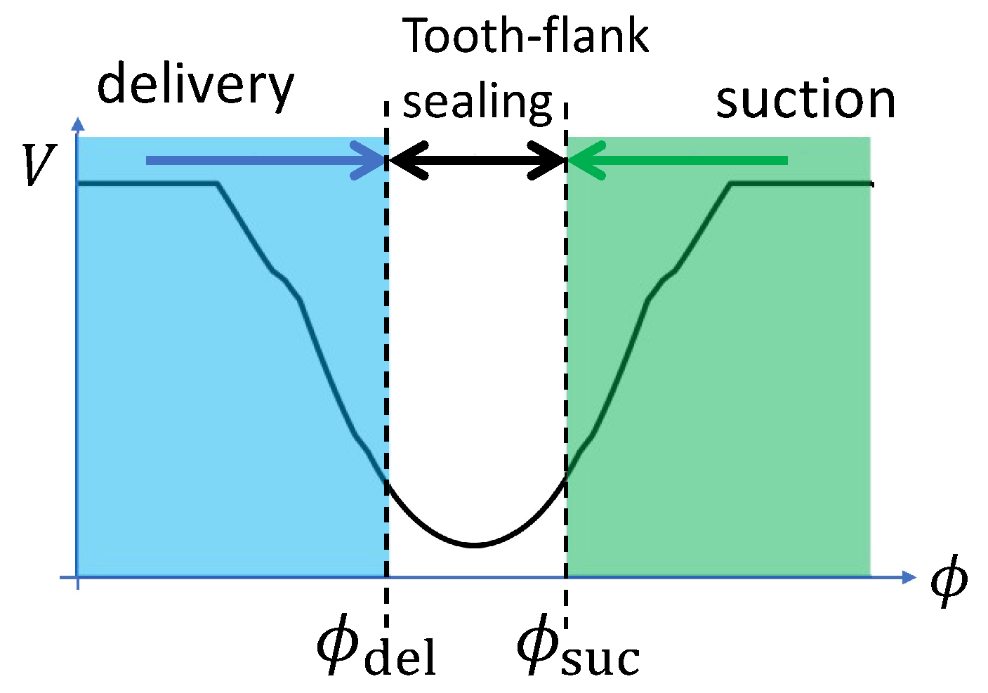
Figure 13.
Zero angle ( = 0) position for a DC of an EGP, where two delimiting contact points have equal distance to the pitch point. The tooth-flank sealing region on the primary line of action is shaded by green.
Figure 13.
Zero angle ( = 0) position for a DC of an EGP, where two delimiting contact points have equal distance to the pitch point. The tooth-flank sealing region on the primary line of action is shaded by green.

Figure 14.
Three volume-curve based porting design: maximum delivery (left), minimum delivery (middle) and intermediate delivery porting design (right).
Figure 14.
Three volume-curve based porting design: maximum delivery (left), minimum delivery (middle) and intermediate delivery porting design (right).

Figure 15.
Examples of groove geometry design for single-flank involute EGPs (a) maximum-delivery (b) minimum-delivery.
Figure 15.
Examples of groove geometry design for single-flank involute EGPs (a) maximum-delivery (b) minimum-delivery.
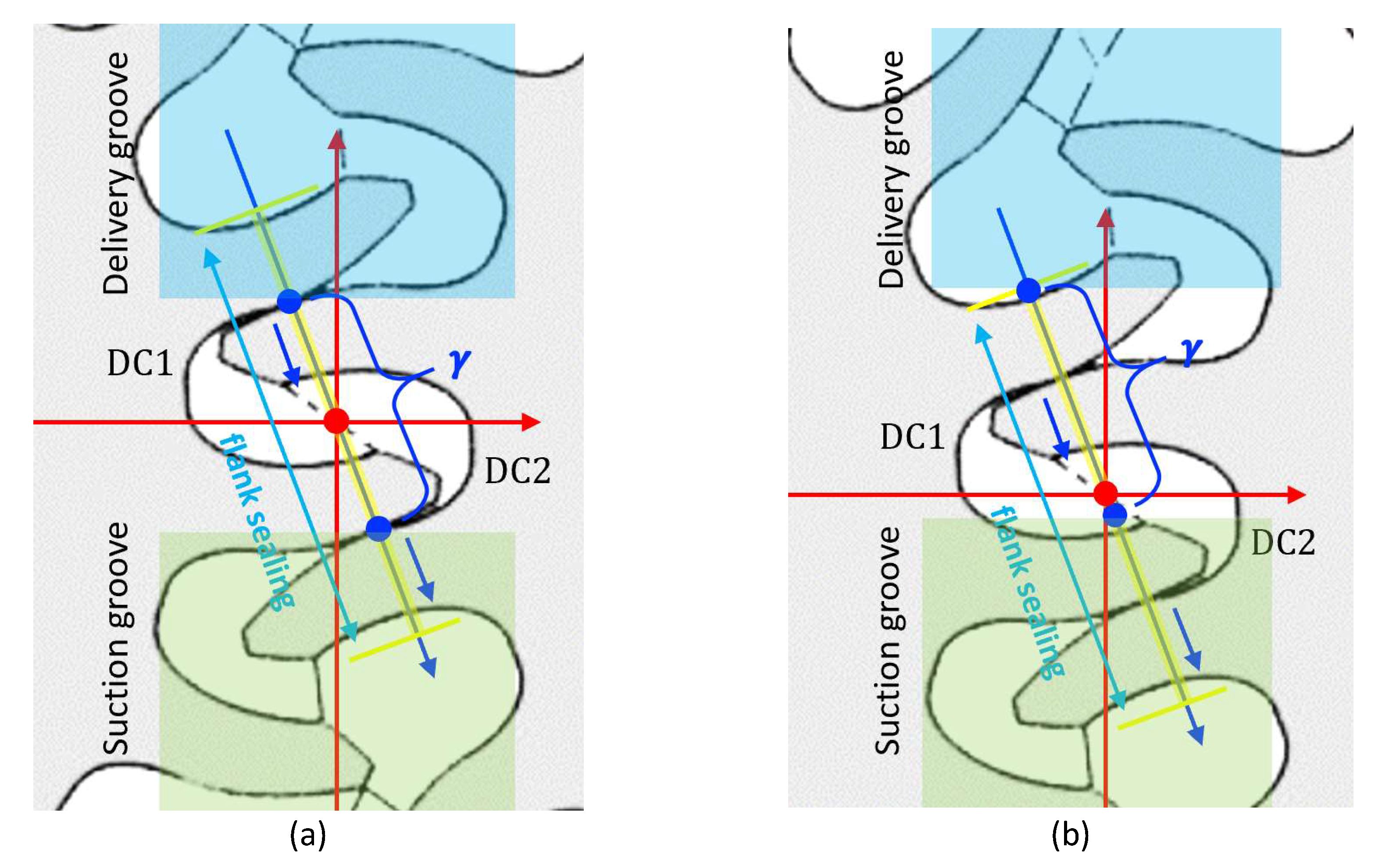
Figure 16.
(a) Kinematic flow ripple (reference design, 2000 RPM) changes with different groove positioning specified by ; (b) the mean flowrate reduction with .
Figure 16.
(a) Kinematic flow ripple (reference design, 2000 RPM) changes with different groove positioning specified by ; (b) the mean flowrate reduction with .

Figure 17.
Fluid dynamic and kinematic flow ripple for the reference pump, assuming the minimum-delivery groove position. The simulation assumes a zero-pressure differential for various shaft speeds.
Figure 17.
Fluid dynamic and kinematic flow ripple for the reference pump, assuming the minimum-delivery groove position. The simulation assumes a zero-pressure differential for various shaft speeds.

Figure 18.
Fluid dynamic and kinematic flow ripple for the reference pump, assuming the maximum-delivery groove position. The simulation assumes a zero-pressure differential for various shaft speeds.
Figure 18.
Fluid dynamic and kinematic flow ripple for the reference pump, assuming the maximum-delivery groove position. The simulation assumes a zero-pressure differential for various shaft speeds.

Figure 19.
Circuit for the displacement solution.

Figure 20.
The change of kinematic ripple under 2000 RPM 200 bar condition for the volume-termination circuit (VT) and for the restriction-termination circuit (RT).
Figure 20.
The change of kinematic ripple under 2000 RPM 200 bar condition for the volume-termination circuit (VT) and for the restriction-termination circuit (RT).

Figure 21.
The hydraulic circuit connection representing the DC pressurization.

Figure 22.
(a) The kinematics of single-DC pressurization problem; (b) Corresponding hydraulic circuit.
Figure 22.
(a) The kinematics of single-DC pressurization problem; (b) Corresponding hydraulic circuit.

Figure 23.
(a) Pressurization solution with = 0.1 and different (b) pressurization solution Q2 with = 5 and different (c) Two time constants and on the pressurization solution at = 0.1 and = 5.
Figure 23.
(a) Pressurization solution with = 0.1 and different (b) pressurization solution Q2 with = 5 and different (c) Two time constants and on the pressurization solution at = 0.1 and = 5.
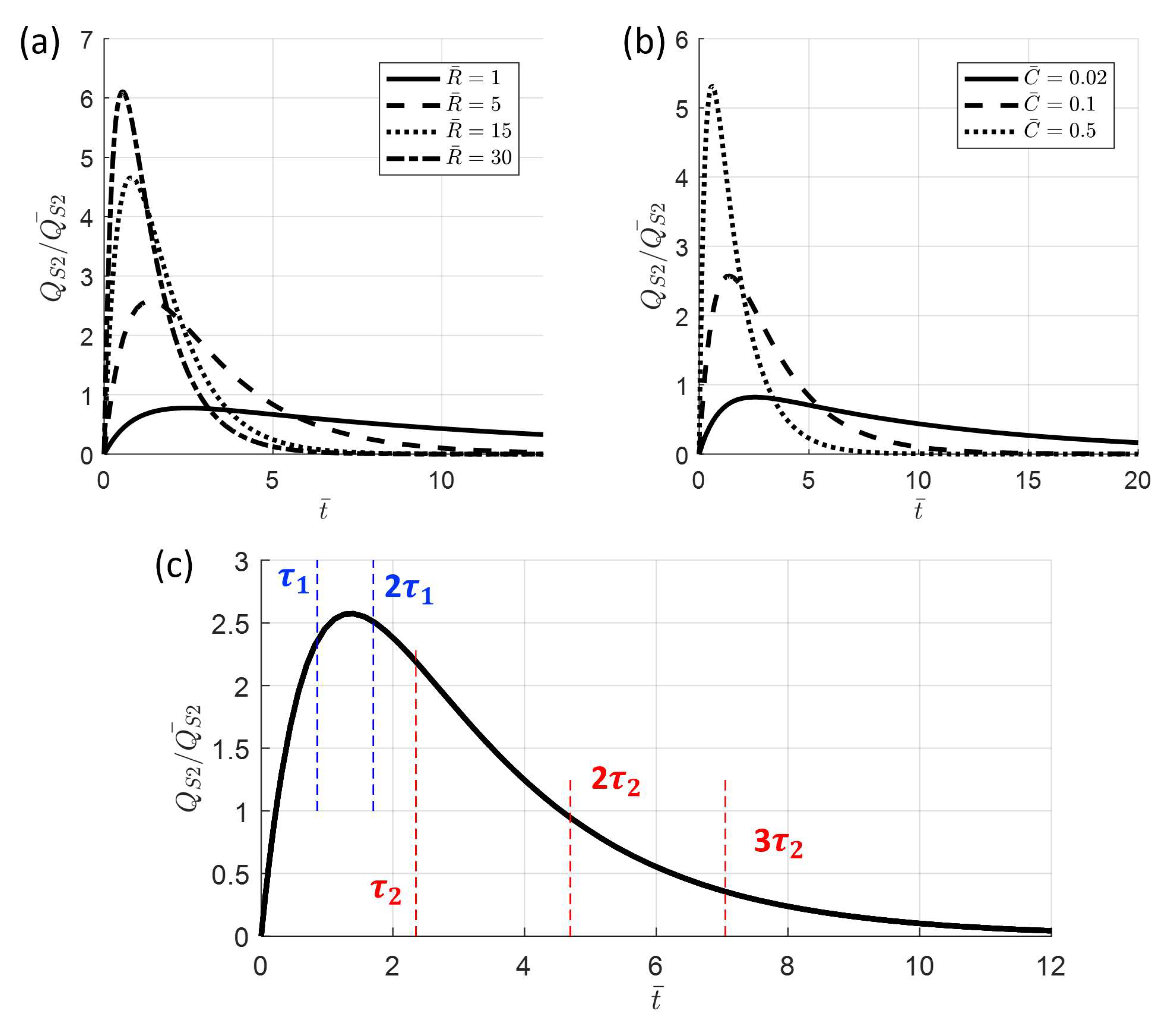
Figure 24.
Recovery of simulated ripple using full hydraulic circuit by adding the kinematic ripple solution and the linearized pressurization ripple solution together for single-DC pressurization problem.
Figure 24.
Recovery of simulated ripple using full hydraulic circuit by adding the kinematic ripple solution and the linearized pressurization ripple solution together for single-DC pressurization problem.

Figure 25.
The four test cases considered for the analysis of the pressurization solution.

Figure 26.
Plots of four pressurization ripple solutions: for the reference gear pump at 2000 RPM, 200 bar. The VT circuit is assumed for four different setups, from C1 to C4. Ripples are plotted in (a) time domain and (b) frequency domain up to 10,000 Hz.
Figure 26.
Plots of four pressurization ripple solutions: for the reference gear pump at 2000 RPM, 200 bar. The VT circuit is assumed for four different setups, from C1 to C4. Ripples are plotted in (a) time domain and (b) frequency domain up to 10,000 Hz.
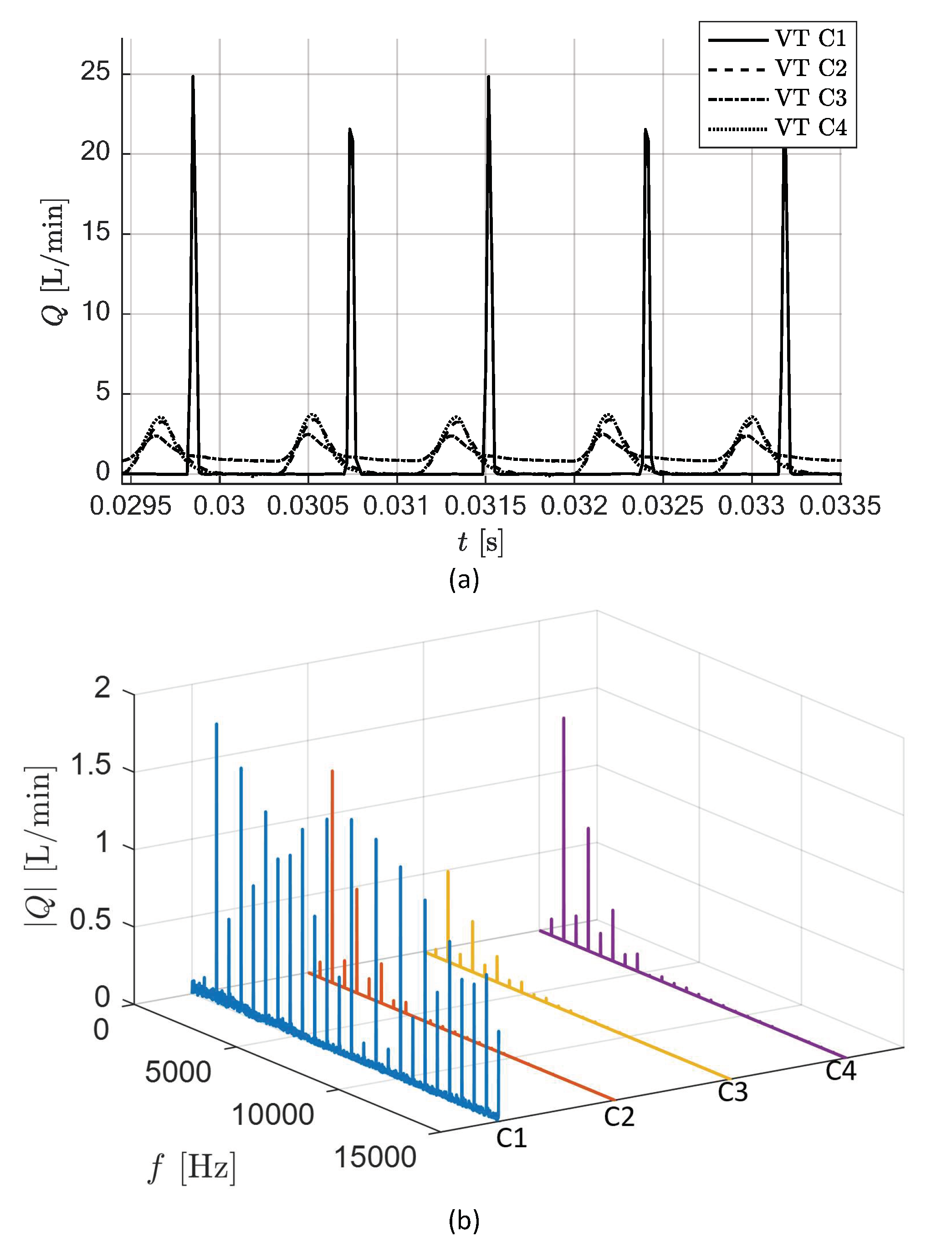
Figure 27.
Plots of four pressurization ripple solutions: for the reference gear pump at 2000 RPM, 200 bar. The RT circuit is assumed for four different setups, from C1 to C4. Ripples are plotted in (a) time domain and (b) frequency domain up to 10,000 Hz.
Figure 27.
Plots of four pressurization ripple solutions: for the reference gear pump at 2000 RPM, 200 bar. The RT circuit is assumed for four different setups, from C1 to C4. Ripples are plotted in (a) time domain and (b) frequency domain up to 10,000 Hz.

Figure 28.
Numerical results of the transfer function for the reference gear pump under four design configurations (from C1 to C4) at 2000 RPM and 200 bar (a) magnitude (b) phase.
Figure 28.
Numerical results of the transfer function for the reference gear pump under four design configurations (from C1 to C4) at 2000 RPM and 200 bar (a) magnitude (b) phase.

Figure 29.
Numerical results of the transfer function for the reference gear pump under four design configurations (from C1 to C4) at 2000 RPM and 100 bar (a) magnitude (b) phase.
Figure 29.
Numerical results of the transfer function for the reference gear pump under four design configurations (from C1 to C4) at 2000 RPM and 100 bar (a) magnitude (b) phase.


Table 1.
Specifications for the gear pump taken as reference in this study.
| Number of teeth | 18 | Drive pressure angle (deg) | 30 |
| Correction factor x | −0.9 | Coast pressure angle (deg) | 15 |
| Addendum radius (mm) | 19.27 | Root radius (mm) | 13.33 |
| Center distance (mm) | 33.36 | Axial length H (mm) | 39 |
| Displacement (cc/rev) | 22.2 | Profile contact ratio | 2.0 |
| Casing opening angle (deg) | 65 | Helical contact ratio | 0 |
| Module (mm) | 2.016 |
© 2019 by the authors. Licensee MDPI, Basel, Switzerland. This article is an open access article distributed under the terms and conditions of the Creative Commons Attribution (CC BY) license (http://creativecommons.org/licenses/by/4.0/).
Share and Cite
MDPI and ACS Style
Zhao, X.; Vacca, A. Theoretical Investigation into the Ripple Source of External Gear Pumps. Energies 2019, 12, 535. https://doi.org/10.3390/en12030535
AMA Style
Zhao X, Vacca A. Theoretical Investigation into the Ripple Source of External Gear Pumps. Energies. 2019; 12(3):535. https://doi.org/10.3390/en12030535
Chicago/Turabian StyleZhao, Xinran, and Andrea Vacca. 2019. "Theoretical Investigation into the Ripple Source of External Gear Pumps" Energies 12, no. 3: 535. https://doi.org/10.3390/en12030535
Note that from the first issue of 2016, this journal uses article numbers instead of page numbers. See further details here.