GA-BP Neural Network-Based Strain Prediction in Full-Scale Static Testing of Wind Turbine Blades

Abstract

This paper proposes a strain prediction method for wind turbine blades using genetic algorithm back propagation neural networks (GA-BPNNs) with applied loads, loading positions, and displacement as inputs, and the study can be used to provide more data for the wind turbine blades’ health assessment and life prediction. Among all parameters to be tested in full-scale static testing of wind turbine blades, strain is very important. The correlation between the blade strain and the applied loads, loading position, displacement, etc., is non-linear, and the number of input variables is too much, thus the calculation and prediction of the blade strain are very complex and difficult. Moreover, the number of measuring points on the blade is limited, so the full-scale blade static test cannot usually provide enough data and information for the improvement of the blade design. As a result of these concerns, this paper studies strain prediction methods for full-scale blade static testing by introducing GA-BPNN. The accuracy and usability of the GA-BPNN prediction model was verified by the comparison with BPNN model and the FEA results. The results show that BPNN can be effectively used to predict the strain of unmeasured points of wind turbine blades.

1. Introduction

Wind turbine blades are one of the core force-bearing components of the wind turbine, and their stability and reliability directly affect the safety of the whole machine. Structural testing is a main way to check the rationality of the design and to verify the safety of manufacturing for turbine blades, and it is also a necessary means to ensure the operational reliability and safety of wind turbines [1]. The purposes of full-scale static testing of wind turbine blades are mainly to obtain two kinds of information from the blade by applying static loads to the blade. One is to verify the blade’s ability under complex design loads, and another is to obtain structural characteristics, such as strain and deformation of the blade. Many studies have been conducted regarding blade structural testing. For example, Fagan et al. [2] presented an experimental testing on a 13-m long wind turbine blade and used the test results to calibrate finite element models, and then the materials used in the blade construction and manufacturing costs were reduced by optimization design using a genetic algorithm. Yang et al. [3] tested the limit loads in full-scale static testing of a wind turbine blade and the deformation situation of the blade under the limit loads. The test results can provide important technical parameters for the blade design. Pan [4] studied the effects of structural non-linearity on the full-scale static testing of wind turbine blades, and analyzed the relationship between bending moment, strain, stiffness, and deflection, and then provided more accurate stiffness data for a numerical model of load calculations for wind turbines. Thus, many achievements have been obtained in the blade load bearing capacity and parameter measurement methods, and some studies have also focused on structural characteristics and damage analysis of the blades [5,6,7,8,9,10,11,12]. Besides, some surrogate models for wind turbine blade stress/strain prediction due to the significant computational burden of physics-based simulation were constructed [13,14]. However, studies on the effects of the applied load, loading positions, and blade displacement on the test results are rare, and in the full-scale static testing of the wind turbine blade, the numbers of measuring points and strain gauges are also limited. Therefore, full-scale static testing only plays a role in the blade certification and has little significance to the blade design [4]. Blade strain is correlated to the applied load, loading position, displacement, etc. If the correlation is neglected, the test environment will have a huge deviation with the actual working conditions and the test result will be unreliable. The relation between blade strain and the applied load, loading position, displacement, etc. is non-linear, and the number of input variables is many, thus, the calculation and prediction of blade train are very complex. Back propagation neural networks (BPNNs) use an error back propagation algorithm to learn and adapt unknown information and has significant advantages in dealing with non-linear fitting and multi-input parameters. Yang et al. [15] showed that BPNNs have a good performance in solving non-linear problems by comparing with other methods in terms of absolute distance as a similarity measure. Moghaddam et al. [16] showed that BPNNs were good at solving non-linear and multi-input parameter problems. The methods of BPNNs were also introduced in the field of wind turbines. Huang et al. [17] applied the BPNN method to vibration fault diagnosis of wind turbine gearboxes and the accurate diagnostic results proved to be effective for analyzing the standard fault samples (training samples) and simulation samples (testing samples). Chen et al. [18] concluded that BPNNs can be effectively utilized to detect the incipient wind turbine faulty condition based on the data collected from wind farm supervisory control and data acquisition. Zhang et al. [19] presents an anomaly identification model for wind turbine state parameters by genetic algorithm back propagation neural network (GA-BPNN). But there are fewer studies about wind turbine blade structures. Liu [20] investigated BPNN control methods for divergent instability based on classical flutter of five degrees of freedom (DOF) wind turbine blade sections driven by pitch adjustment, and the obvious effects of fuzzy control and BPNN control are illustrated by numerical comparisons of vibration suppression from non-linear time response, amplitude of LCO, and frequency spectrum analysis.

Compared with traditional BPNN methods, BPNNs improved by genetic algorithm (GA-BPNNs) can find better initial weight and threshold and avoid falling into local optimal situations, which traditional BPNNs often meet. Moreover, the systems constructed by GA-BPNNs have better robustness and applicability in dealing with complex problems [21]. Therefore, taking the advantages of the neural network in dealing with non-linear fitting and multi-input parameters, a strain-predictive GA-BPNN model for the full-scale wind turbine blades static testing was established, and the strain value prediction of the unmeasured points was realized. The accuracy of the GA-BPNN prediction model was verified by comparison with BPNN model and FE analysis results. The applicability and usability of a neural network prediction model was verified by comparing the prediction results with the ANSYS simulation data. The study can provide the basis for the design and calibration of wind turbine blades.

The remainder of this article is designed as follows. In Section 2, the basic concepts of neural networks and the basic framework and algorithms of GA-BPNNs are introduced. The conditions and test procedures for the full-scale wind turbine blades static testing are introduced in Section 3. In Section 4, firstly, a strain-predictive GA-BPNN model was established for the center and trailing edge of the suction side based on a full-scale static testing. Secondly, the accuracy of the strain–predictive GA-BPNN model was verified by comparison with that of BPNN and FE analysis results. Then, the strain on the positions of the maximum chord length, the gravity center, and the root of the wind turbine blade are predicted. Finally, the reliability and applicability of the proposed model are proved by comparing with the ANSYS simulation result. Ultimately, conclusions are dawn in Section 5.

2. The Method of GA-BPNN

2.1. The Principles of BPNN

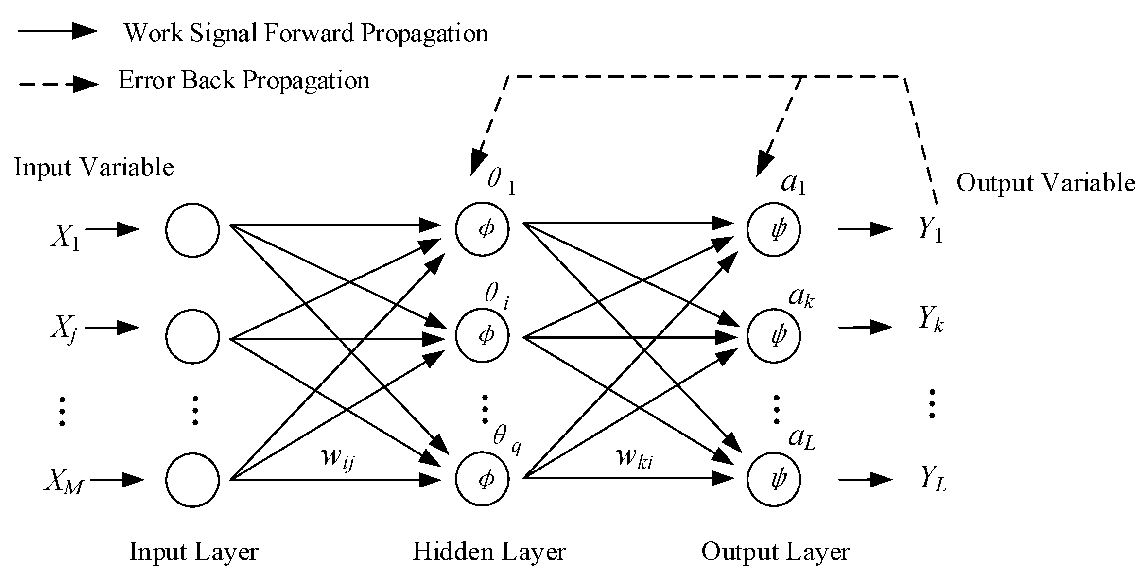
A relational model between the input set {X_j|j = 1,2,…,M} and the dependent variable Y was established using the improved neural network algorithm. Sample X₁,…,X_M was used as the input value and Y₁,…,Y_L was the output value for training the dependent variable prediction model. The BPNN builds the network structure of the strain–prediction model for the full-scale wind turbine blade static testing, as shown in Figure 1.

In Figure 1, $X_i$ represents the input of the j-th node of the input layer, $j=1,2,\cdots ,m$; $w_{ij}$ represents the weight value between the i-th node of the hidden layer and the j-th node of the input layer; and ${\theta }_i$ represents the threshold value of the i-th node of the hidden layer. $\varphi \left(x\right)$ represents the excitation function of the hidden layer; $w_{ki}$ represents the weight between the k-th node of the output layer and the i-th node of the hidden layer, $i=1,2,\cdots ,q$; $a_k$ represents the threshold value of the k-th node of the output layer, $k=1,2,\cdots ,l$; $\psi \left(x\right)$ represents the excitation function of the output layer; $Y_k$ represents the output of the k-th node of the output layer. The data about the location of strain gauge, the loads with different percentage, and the displacement of loading positions were used as input data, and the data about strains and stresses were used as output data.

2.2. The Principles of GA-BPNN

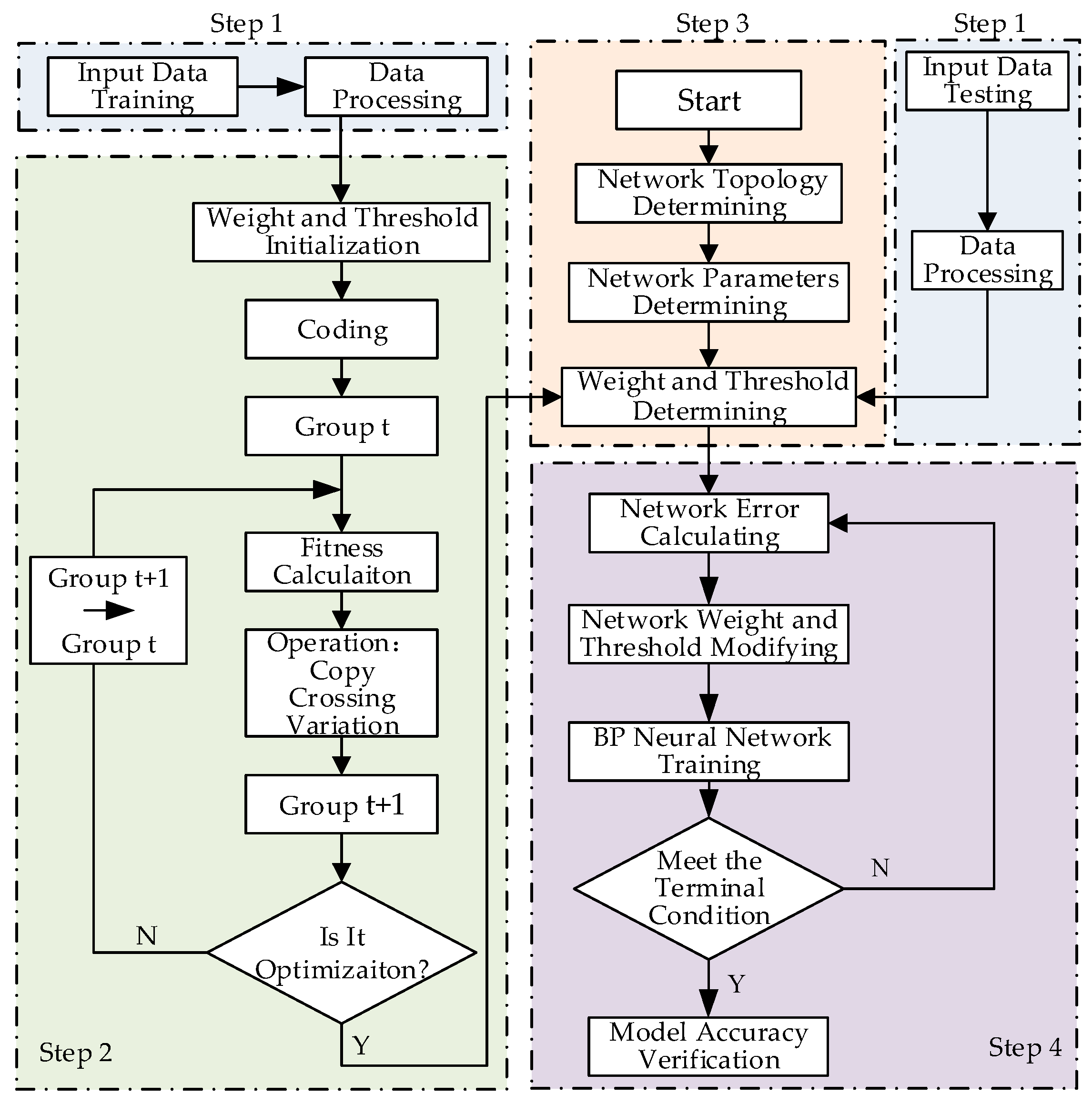
Since the gradient descent method is used by BPNN algorithms, it is easy to fall into a situation of local optimization. Using a genetic algorithm to optimize the weight and threshold of BPNNs, which is improved by the Levenberg–Marquardt formula, can minimize the training error of the neural network, which can effectively avoid the training falling into a local optimization situation [22,23]. The weight and threshold of the BPNN are the chromosomes of the genetic algorithm. Each element of a chromosome is called a gene. The chromosomes with poor fitness values are eliminated, and the best genomes are selected to obtain the optimal solution by calculating the fitness values of each chromosome continuously. The method of BPNN improved on the basis of the genetic algorithm is shown in Figure 2 [24,25].

Step 1: Data processing. The input and output variables are determined. The input data are trained to speed-up network calculating.

Step 2: The weight and threshold are optimized. (1) The evolution numbers, population size, crossover probability, and mutation probability are initialized. (2) The network weight and threshold are encoded, and the fitness function, which is the reciprocal of the sum of errors squared is determined. (3) The selection operation: the chromosome with the fitness value “good” from the current population is selected as the parent. The higher the individual fitness value is, the greater the probability of the chromosome selected. The roulette method is used to select chromosomes. That is, a uniformly distributed random number is generated in [0, 1], and if r ≤ q₁, the chromosome x₁ is selected. If q_k–1 < r ≤ q_k (2 ≤ k ≤ N), the chromosome x_k is selected, and q_i is called the accumulation probability of chromosome x_i (i = 1,2,…,n), and its calculation formula is as shown in Equation (1). (4) Cross: two chromosomes are selected according to a certain probability, one or more points in the two chromosomes are exchanged with each other randomly to obtain two new chromosomes. (5) Variation: according to a certain mutation probability, in the binary coding of chromosomes, 1 becomes 0, and 0 becomes 1. This operation can effectively avoid premature convergence in the evolution process and thus falling into a local optimum. (6) Repeat steps (3), (4), and (5) until the number of evolutions is reached, then the optimal weights as well as the thresholds will be obtained.

Step 3, the BPNN model is built. The optimal initial weights and thresholds are obtained to construct the BPNN [25]. Any non-linear mapping can be realized by the three-layer BPNN in theory. The hidden-layer number, number of times, step size, and target of the BPNN are constructed. A tangent S-type transfer function as Equation (2) is used between the input layer and the hidden layer, while a linear transfer function as Equation (3) is used between the hidden layer and the output layer.

Step 4: the results are obtained by BPNN. The sample data are inputted into the BPNN model to predict the output data and then the output data are obtained if the results meet the terminal condition.

$$q_i={\displaystyle \sum _{j=1}^{i}P(x_j)}$$

(1)

$$f(x)=\frac{1}{1+e^{-x}}$$

(2)

$$f(x)=kx$$

(3)

3. Full-Scale Static Test of Wind Turbine Blades

3.1. The Wind Turbine Blade Specification

The full-scale static testing was conducted in cooperation with a certain blade company, and the testing result was used to verify the safety of the blade prototype, and was also used for further improvement. The testing process followed GB/T 25384-2010 [26].

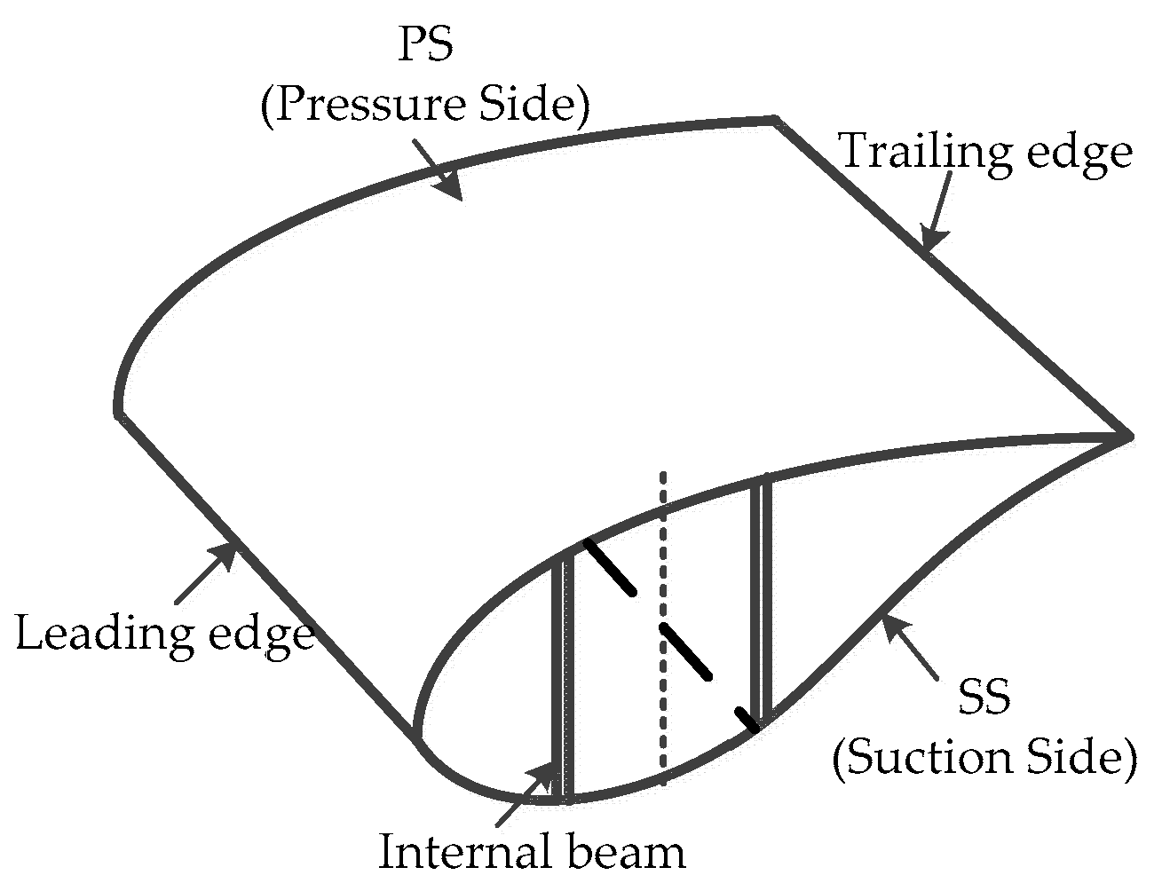
The blade prototype was mainly made of fiber reinforced polymer. The blade had a mass of 15,968 kg and a natural frequency of 1.41 Hz. The maximum chord length was 3.8 m. The main elements of a wind turbine blade are shown in Figure 3.

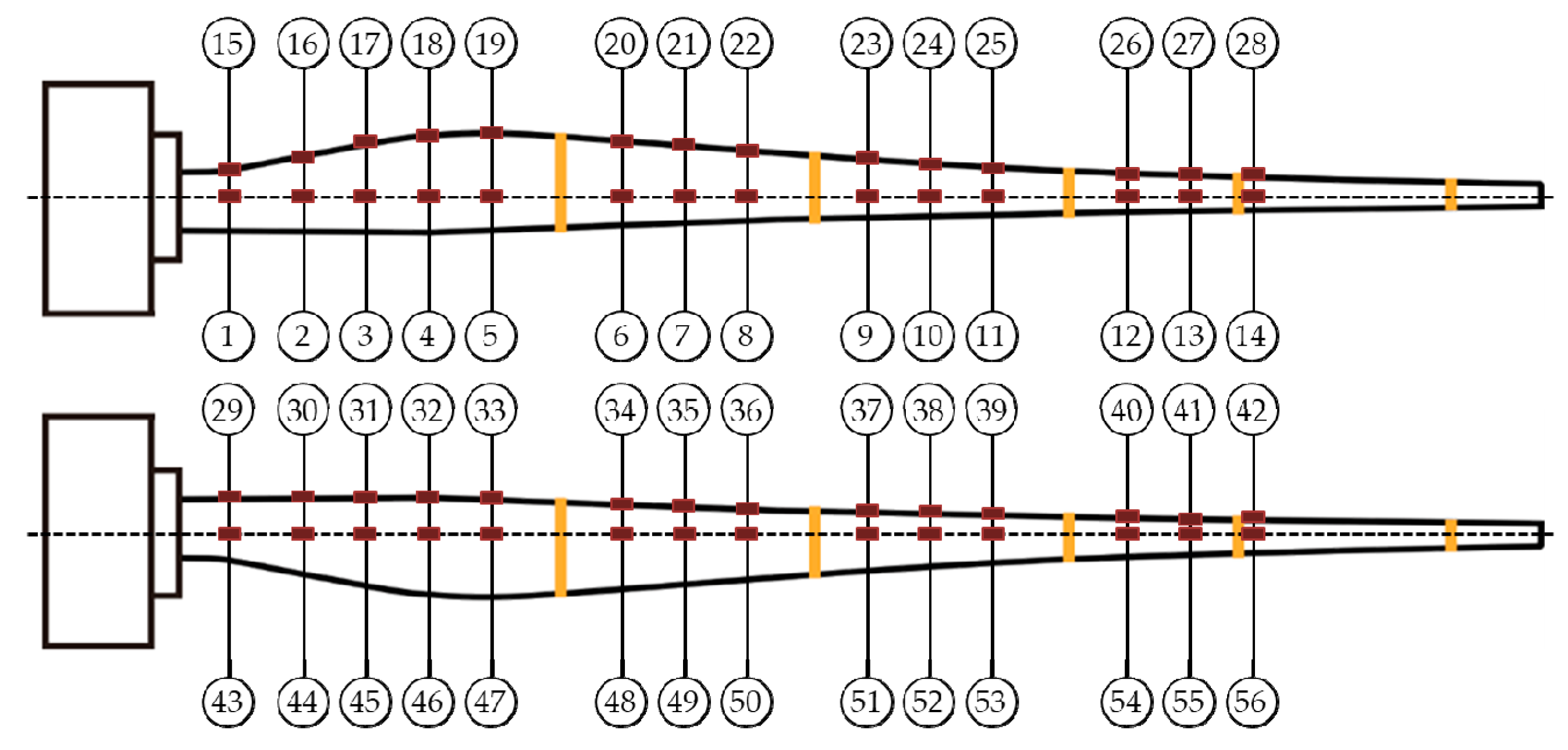
In the full-scale static testing, 56 strain gauges were attached to the surface of the wind turbine blade on the center of the pressure side (PS), the center of suction side (SS), the leading edge, and the trailing edge before testing. The locations and positions of strain gauges attached on the blade are shown in Figure 4.

3.2. Testing Procedure

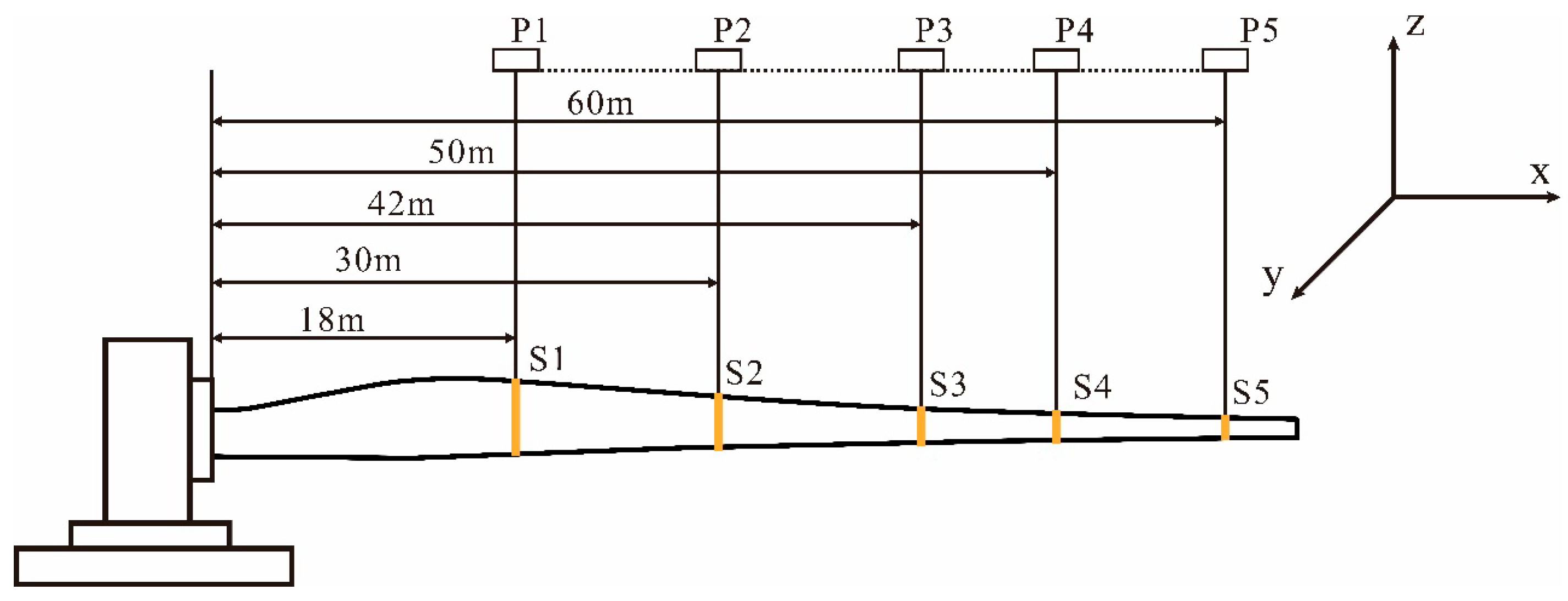
The blade is fixed to the test platform by 64 bolts on the blade root, the limit loading was performed by pulling from one side, and the applied loading diagram is shown in Figure 5, where P1‒P5 are the positions of the tensile machine, S1‒S5 are the load application points. From Figure 5, we can see that the loading points were respectively arranged at a distance of 18.00 m, 30.00 m, 42.00 m, 50.00 m, and 60.00 m from the root of the blade, and the loading direction was perpendicular to the normal direction of the loading section.

As this paper aims at proposing a strain–predictive method, it only considers the situation of static testing in the flap+ direction as an example. The structure of every cross-section is different, thus their load bearing capacity is different. The target load of each loading point in the static testing was the design load which was obtained by finite element analysis (FEA) during the initial phase of design, and the applied target load had a certain deviation from the design value for existing equipment loading errors. In the direction of the flap+, the target load of each loading point is shown in

Table 1. The target load of each loading point.

Items	The Distance of Loading Positions from the Blade Root (m)
	18.0	30.0	42.0	50.0	60.0
target load (kN)	94.6	143.0	59.8	104.4	68.0

. Following the test process of GB/T 25384-2010, the applied load, displacement, and strain of the blade were cleared before starting the test. Then, using the lateral loading device, the blade was loaded step by step according to 0%, 40%, 60%, 80%, and 100% of the target load, and the data was recorded. The load of each stage is shown in

Table 2. The applied load of each stage in flap+.

The Applied Load (kN)
The Distance of Loading Positions from the Blade Root (m)	0	40%	60%	80%	100%
18.00	0	37.85	57.48	75.76	94.74
30.00	0	57.42	86.17	114.60	143.15
42.00	0	24.09	35.85	48.16	60.15
50.00	0	42.34	62.75	83.04	104.67
60.00	0	27.25	40.98	54.51	68.07

. The duration of each stage of load was not less than 10 s. After the loading was completed, the unloading was performed step by step, the blade load was unloaded to the zero state, and the displacement data and the strain gauge data were recorded during the loading process.

4. GA-BPNN-Based Strain Prediction in Full-Scale Static Testing

4.1. GA-BPNN-Based Strain Prediction for the Center of Suction Side

During the loading process of the full-scale static testing, there was a non-linear mapping relationship between the strain and the applied load, loading positions, and displacements. The neural network, with its good learning method, can approximately express the non-linear mapping relationship between the above parameters through the establishment of the network model. Thereby, the strain of the blade is predicted. In the GA-BPNN model for strain prediction, the applied load, the loading positions, and the displacements were used as training inputs, and the strain of wind turbine blade was output. In the full-scale static test, there were 56 sets of data which all come from actual strain gauges, 50 set of data were trained to construct the NN models, while the remaining six sets of data were used to test the model accuracy, then a GA-BPNN model for wind turbine blade strain prediction was established. The training samples and test samples of the GA-BPNN are shown in

Table 3. The training samples of the GA-BPNN.

Items	The Location of Strain Gauge	Load (kN)					The Distanceto the Blade Root (m)
		F1	F2	F3	F4	F5	l1
1	2000	37.85	57.42	24.09	42.34	27.25	0
2	6000	57.48	86.17	35.85	62.75	40.98	1.16
3	9000	75.76	114.6	48.16	83.04	54.51	5.69
…	…	…	…	…	…	…	…
…	…	…	…	…	…	…	…
50	48,000	75.76	114.6	48.16	83.04	54.51	5.69
Items	The Displacement of Loading Positions (m)
	s1	s2	s3	s4	s5	s6	s7
1	159	755	2159	3717	6384	7900	−1186
2	264	1158	3257	5596	9605	11,876	−1898
3	368	1557	4350	7469	12,773	15,770	−2383
…	…	…	…	…	…	…	…
…	…	…	…	…	…	…	…
50	368	1557	4350	7469	12,773	15,770	−2971

and

Table 4. The test samples of the GA-BPNN.

Items	The Location of Strain Gauge	Load (kN)					The Distanceto the Blade Root (m)
		F1	F2	F3	F4	F5	l1
1	2000	57.48	86.17	35.85	62.75	40.98	1.16
2	15,000	75.76	114.6	48.16	83.04	54.51	5.69
3	24,000	37.85	57.42	24.09	42.34	27.25	0
4	36,000	94.74	143.15	60.15	104.67	68.07	8.51
5	51,000	75.76	114.6	48.16	83.04	54.51	5.69
6	33,000	57.48	86.17	35.85	62.75	40.98	1.16
Items	The Displacement of Loading Positions (m)
	s1	s2	s3	s4	s5	s6	s7
1	264	1158	3257	5596	9605	11,876	−1790
2	368	1557	4350	7469	12,773	15,770	−2748
3	159	755	2159	3717	6384	7900	−1964
4	477	1976	5490	9405	16,019	19,741	−4849
5	368	1557	4350	7469	12,773	15,770	−2490
6	264	1158	3257	5596	9605	11,876	−3047

, respectively. The measurement method was up to standard. According to the test program, 14 strain gauges were arranged in the center of the suction side and the target load was imposed gradually by four steps with the duration of every step more than 10 s, thus 56 sets of data were obtained in the four different cases. Since the BPNN model needed enough training samples to ensure effectiveness, and the data used to test could not be selected as training data, the sample size of test data should try to be minimized without too much manual interference, so six samples were randomly selected as the test samples.

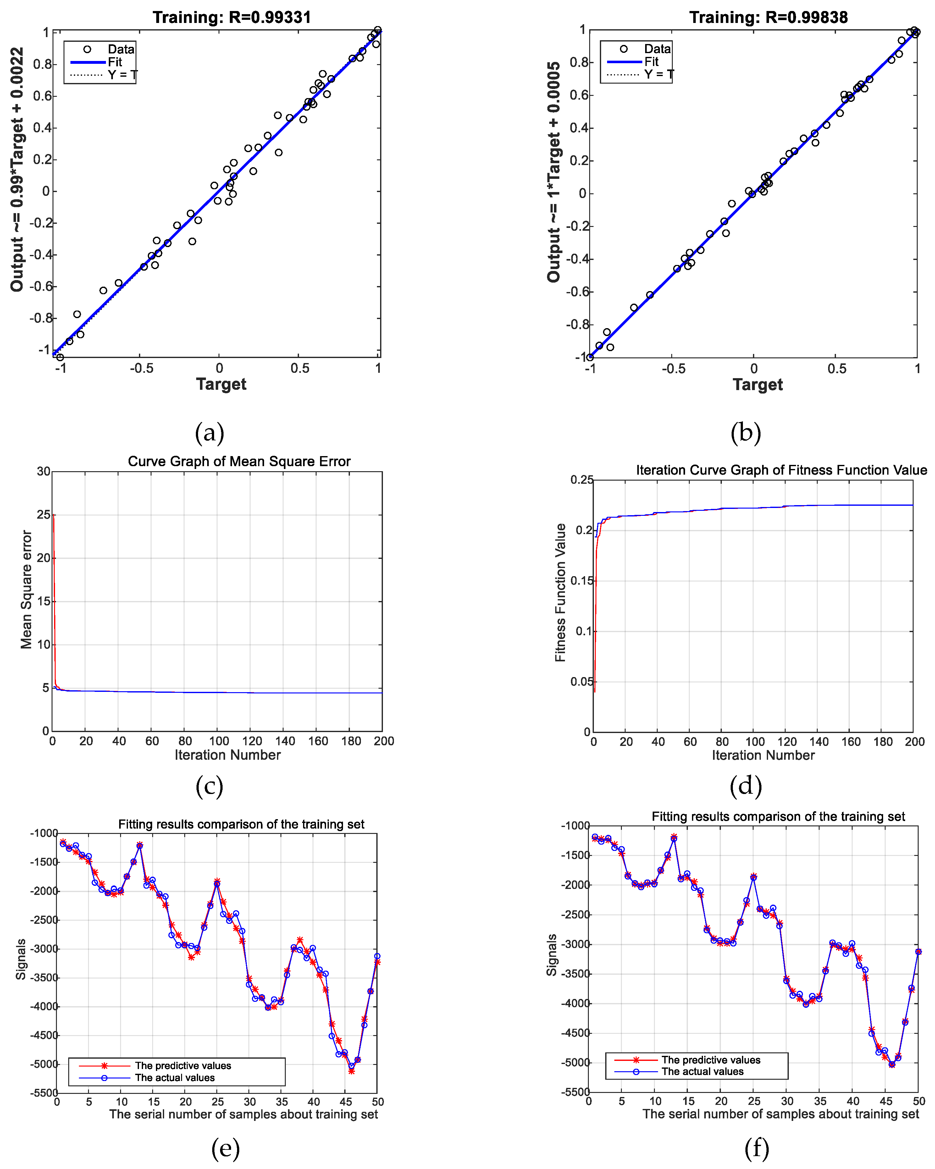
The specific procedure of the GA-BPNN is set as follows: The input dimension is 13, and the output dimension is 1. Seven neurons are set in the hidden layer, and a tangent S-type transfer function such as Equation (2) was used between the input layer and the hidden layer. A linear transfer function such as Equation (3) between the hidden layer and the output layer was used. The network maximum number of training steps was 2000 steps, the network learning rate was six, the momentum factor is one, the training target was allowed to have a minimum convergence error of le-3, and the training result were displayed at intervals of 50 steps. The learning process of the training samples was simulated. Set the genetic algorithm population size to 1800 and the genetic iteration to 200. Call the GAOT which is the genetic algorithm toolbox in MATLAB and get the predicted correlation values. In order to verify the accuracy and validity of the GA-BPNN, traditional BPNN was also used to predict the strain. The specific procedure of the BPNN was set as follows: The input dimension was 16, and the output dimension was 1. There were seven neurons in the hidden layer, with a tangent S-type transfer function between the input layer and the hidden layer. In addition, a linear transfer function between the hidden layer and the output layer was used. The network maximum number of training steps was 2000 steps, the network learning rate was two, the training target was allowed to have a minimum convergence error of le-3, and the training result was displayed at intervals of 50 steps. The learning process of the training samples was simulated. The comparison results are shown as Figure 6.

Figure 6a,b shows regression curve of BPNN model error and GA-BPNN model error, respectively. In Figure 6a, it shows regression analysis of the training samples by BPNN model, the relevant regression coefficient was 0.99331, The relevant regression coefficient was good, which means strain prediction in full-scale static testing of wind turbine blades has good performance based on BPNN. However, Figure 6b shows that the relevant regression coefficient of GA-BPNN was 0.99838, the relevant regression coefficient was closer to 1. Figure 6c is the curve graph of mean square error, where the blue line represents the minimum sum of squared errors and the red line represents the sum of squared errors; Figure 6d is the iteration curve graph of the fitness function value, the best fitness function value is shown by a blue line, whereas the average fitness function value is shown by a red line. The genetic algorithm runs 200 times during an iteration step. In addition, from Figure 6e,f, the curve of the prediction values fitted by GA-BPNN was more similar to that of the actual values than BPNN, so we can conclude that the fitting results of GA-BPNN were better than BPNN, which means GA-BPNN has a better performance than BPNN. From

Table 5. The input weight values of the BPNN.

−1.624	−0.512	−0.417	−0.084	−0.001	0.320	0.260	0.712	0.008	0.111	−0.382	−0.780	0.660
−0.444	−0.136	0.609	−0.492	−0.509	−0.182	−0.598	−0.761	−0.186	−0.243	−0.786	−0.296	−0.198
0.752	0.050	−0.181	0.496	0.566	0.578	−0.792	−0.285	−0.212	−0.684	−0.236	−0.142	−0.203
0.958	−0.057	0.577	−0.194	0.442	0.591	−0.815	−0.558	−0.676	0.162	0.675	0.206	0.091
−0.635	−0.264	0.651	−0.449	0.632	0.333	0.226	0.340	−0.109	−0.219	0.298	−0.844	0.505
0.217	0.182	0.478	−0.769	0.072	−0.530	0.283	−0.203	−0.106	0.436	0.570	−0.286	−0.373
1.450	−0.685	0.204	0.173	0.117	−0.745	−0.620	0.052	0.535	−0.263	0.598	−0.487	−0.182

and

Table 6. The input weight values of the GA-BPNN.

−3.288	0.581	−0.291	−0.754	−0.506	0.911	0.032	−0.245	0.185	−0.532	−0.308	0.648	0.230
−2.997	0.292	−0.991	−0.479	0.125	0.2931	−0.114	−0.357	−0.606	1.1067	−0.465	0.768	0.473
0.188	−0.658	−0.602	−0.798	0.145	−1.308	−0.993	−0.486	−0.466	−1.517	0.0098	0.063	0.233
0.115	0.649	−0.239	−0.401	0.574	−0.624	−0.898	−0.949	−0.045	0.681	−0.834	−0.593	−0.559
−0.840	0.154	−0.366	1.023	0.784	−0.651	−0.378	0.3140	0.922	0.233	−0.807	−0.184	−0.164
−2.537	0.575	−0.386	0.625	0.151	−0.056	−0.062	−0.721	−0.067	−0.654	0.579	−0.715	0.440
0.415	1.046	0.047	−0.508	1.002	−0.638	−0.023	−0.274	−0.669	−0.590	0.483	0.112	0.636

, the input weighting values of the traditional BPNN method and the GA-BPNN method have been presented, respectively. The input weighting values were a 13 × 7 matrix because of the input data with 13 variables and the 7 hidden-layer nodes and all of the BPNN and GA-BPNN were set this way.

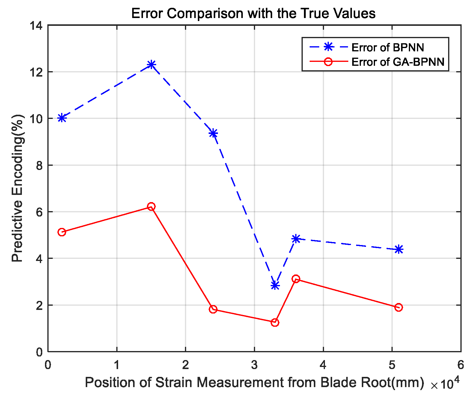
The test sample was used to verify the recognition ability of the GA-BPNN compared with the traditional BPNN, the comparison results are shown as Figure 7. The errors are calculated by difference between the true values which were used as testing samples and the predictive values which were trained by GA-BPNN and BPNN, respectively. It can be seen from Figure 7 that the GA-BPNN corresponding to the variable forecasting results were much more accurate, and the relative error rate of the test sample output was within 6.5%. Moreover, the relative error of every test sample analyzed by GA-BPNN was less than those analyzed by BPNN. So, GA-BPNN was more accurate than BPNN.

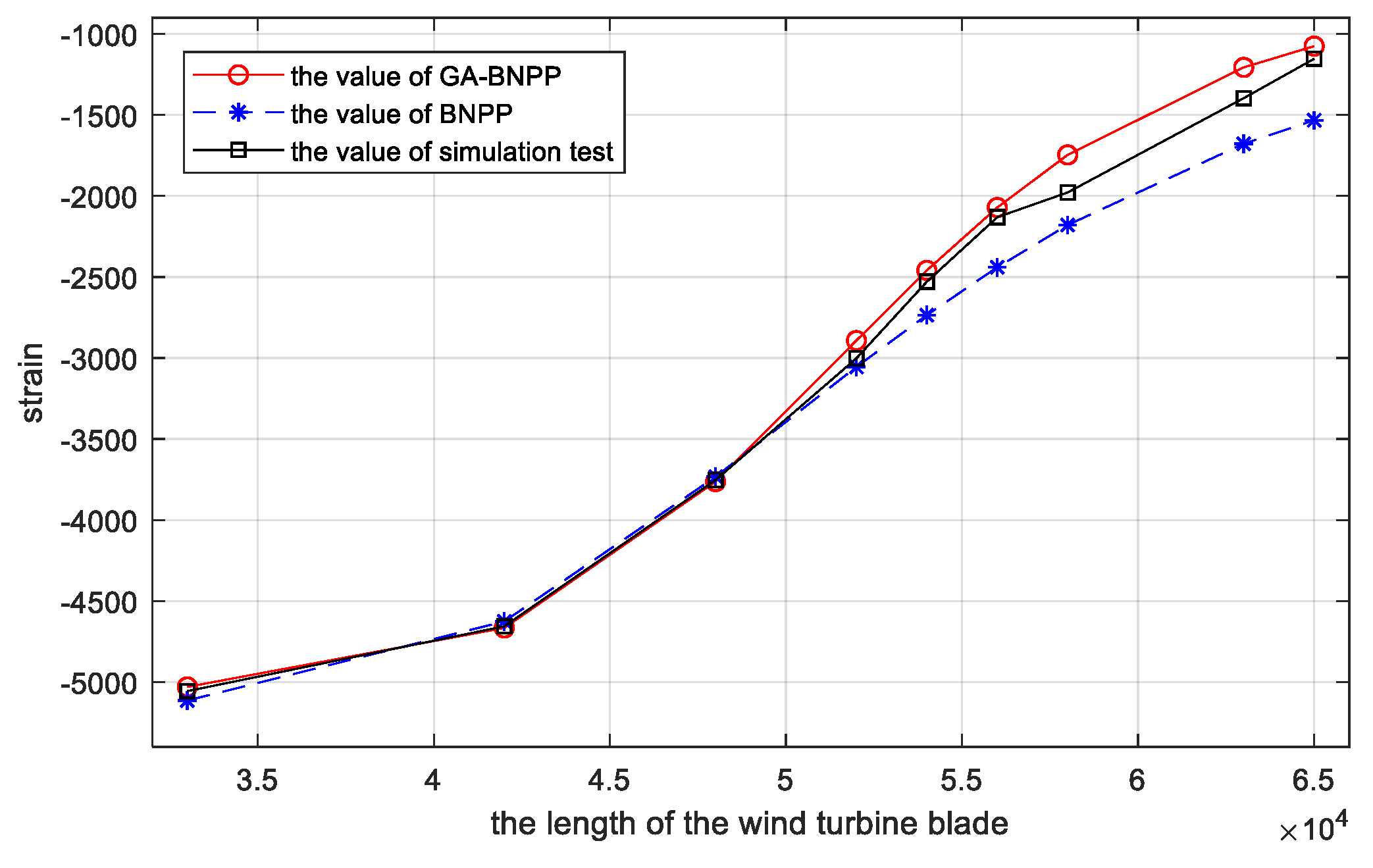
In order to verify the reliability and availability of the BPNN and GA-BPNN, the prediction results were used to compare it with the simulation data made by ANSYS. The unmeasured points on the center of the suction side at 33.00 m, 42.00 m, 48.00 m, 52.00 m, 54.00 m, 56.00 m, 58.00 m, 63.00 m, and 65.00 m from the root of the blade were chosen to predict their strain by using BPNN. Comparing the prediction data with the simulation data, the comparison results are shown in Figure 8. It can be seen from Figure 8 that both BPNN and GA-BPNN have a high accuracy to predict the strain, and that the GA-BPNN had a smaller error.

4.2. GA-BPNN-Based Strain Prediction for the Trailing Edge

As the same with the previous approaches in Section 4.1, the strain forecasting model based on GA-BPNN for the trailing edge was established by GA-BPNN. The training samples and test samples of the GA-BPNN are shown in

Table 7. The training samples of the GA-BPNN.

Items	The Location of Strain Gauge	Load (kN)					The Distanceto the Blade Root (m)
		F1	F2	F3	F4	F5	l1
1	2000	37.85	57.42	24.09	42.34	27.25	0
2	6000	57.48	86.17	35.85	62.75	40.98	1.16
3	9000	75.76	114.6	48.16	83.04	54.51	5.69
…	…	…	…	…	…	…	…
…	…	…	…	…	…	…	…
50	48,000	75.76	114.6	48.16	83.04	54.51	5.69
Items	The Displacement of Loading Positions (m)
	s1	s2	s3	s4	s5	s6	s7
1	159	755	2159	3717	6384	7900	−146
2	264	1158	3257	5596	9605	11,876	−418
3	368	1557	4350	7469	12,773	15,770	−497
…	…	…	…	…	…	…	…
…	…	…	…	…	…	…	…
50	477	1976	5490	9405	16,019	19,741	−396

and

Table 8. The test samples of the GA-BPNN.

Items	The Location of Strain Gauge	Load (kN)					The Distanceto the Blade Root (m)
		F1	F2	F3	F4	F5	l1
1	24,000	37.85	57.42	24.09	42.34	27.25	0
2	21,000	75.76	114.6	48.16	83.04	54.51	5.69
3	33,000	37.85	57.42	24.09	42.34	27.25	0
4	36,000	94.74	143.15	60.15	104.67	68.07	8.51
5	21,000	94.74	143.15	60.15	104.67	68.07	8.51
6	24,000	75.76	114.6	48.16	83.04	54.51	5.69
Items	The Displacement of Loading Positions (m)
	s1	s2	s3	s4	s5	s6	s7
1	159	755	2159	3717	6384	7900	−189
2	368	1557	4350	7469	12,773	15,770	−532
3	159	755	2159	3717	6384	7900	−147
4	477	1976	5490	9405	16,019	19,741	−652
5	477	1976	5490	9405	16,019	19,741	−717
6	368	1557	4350	7469	12,773	15,770	−598

, respectively.

The comparison results of the GA-BPNN and traditional BPNN for the strain prediction of the full-scale static testing of the wind turbine blade are shown as Figure 9.

Figure 9a,b show the training state of BPNN and GA-BPNN, respectively; Figure 9c,d show the regression of BPNN and GA-BPNN, respectively; Figure 9e is the curve graph of mean square error, where the blue line represents the minimum sum of squared errors and the red line represents the average sum of squared errors; Figure 9f is the iteration curve graph of fitness function value, where the best fitness function value is shown by a blue line, whereas the average fitness function value is shown by a red line.

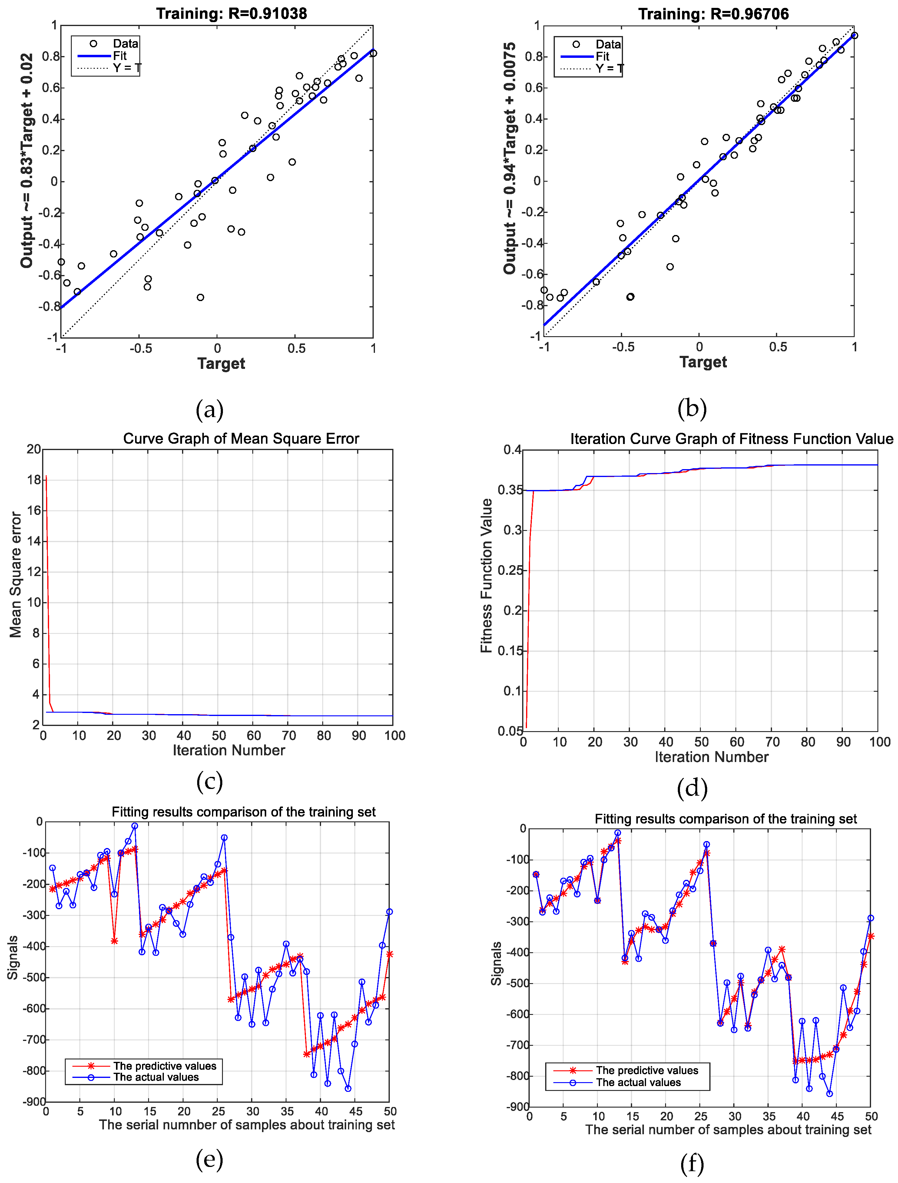
Figure 9a,b show the regression curve of BPNN model error and GA-BPNN model error, respectively. In Figure 9a, it is regression analysis of training samples by the BPNN model, the relevant regression coefficient was 0.91038, the training result is modest according to the relevant regression coefficient. The regression results trained by the BPNN are more different than the theoretical values compared with the regression results from the center of suction side. The reason for this result is that the trailing edge is the joint of two different materials. In Figure 9b, the relevant regression coefficient of GA-BPNN was 0.96706, which is closer to 1, and the number of relevant regression coefficients of GA-BPNN training was bigger than that of the BPNN, which means the regression results of the GA-BPNN was better than the BPNN. In addition, from Figure 9e,f, the fitting results of the GA-BPNN were better than the BPNN, so the GA-BPNN training had the better performance than the BPNN training. From

Table 9. The input weight values of the BPNN.

0.182	0.134	−0.272	−1.017	−1.216	−0.874	−1.074	−0.827	−0.489	−0.865	−0.668	0.041	0.167
−0.216	1.769	2.422	1.784	1.773	2.682	1.436	1.961	1.403	1.449	1.070	1.780	2.273
0.0524	−0.305	0.762	−0.029	−0.317	−0.078	−0.368	0.324	−0.364	0.009	−0.116	0.725	−0.416
−0.317	2.778	1.776	3.031	1.922	3.017	2.795	2.940	2.743	2.104	2.824	2.203	2.066
0.115	−1.131	−0.772	−0.829	−0.806	−0.417	−1.82	−0.654	−1.715	−1.022	−1.058	−0.487	−1.129

and

Table 10. The input weight values of the GA-BPNN.

41.803	−0.991	−1.52	−0.70	2.601	−1.894	0.510	1.772	1.574	0.787	0.038	−1.27	−1.056
0.763	−0.671	−0.05	0.95	−1.021	−0.596	11.960	−0.777	0.365	−0.601	−1.262	−1.40	0.277
−1.333	2.607	1.381	1.42	3.559	0.850	−15.57	3.153	3.654	2.847	2.374	3.27	2.519
−28.76	5.738	4.997	4.46	6.254	5.188	5.005	5.217	6.533	5.527	5.109	4.64	5.508
1.322	3.529	3.600	2.85	−8.248	3.232	3.252	−4.561	−4.716	−3.261	−2.641	1.17	1.212

, the input weighting values of the traditional BPNN method and the GA-BPNN method are presented, respectively. The input weighting values are a 13 × 5 matrix because of the input data with 13 variables and the five hidden-layer nodes, and all of the BPNN and GA-BPNN models were set by this way.

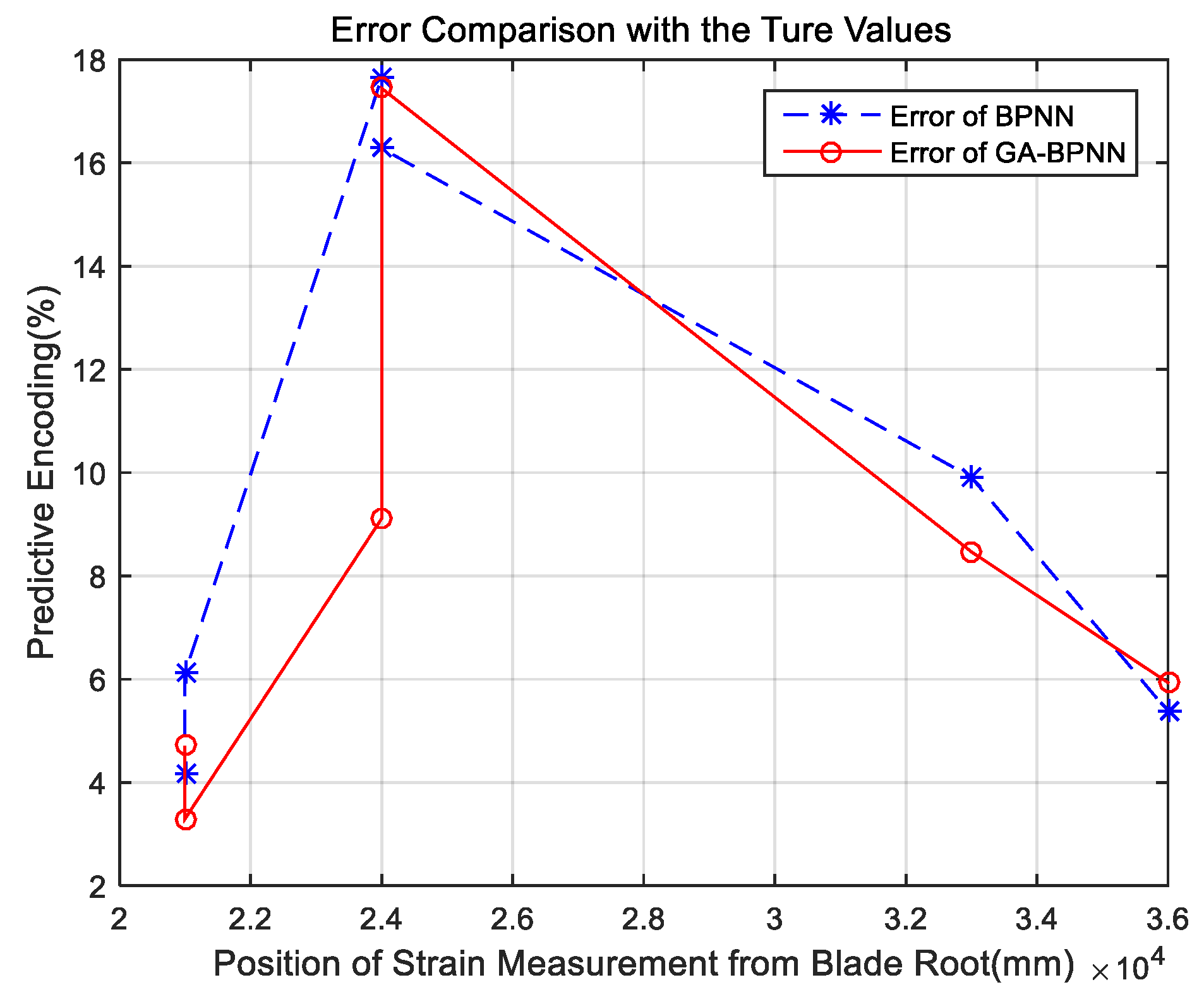
The test sample was used to verify the recognition ability of the GA-BPNN in contrast to traditional BPNN, and the test results were compared as shown in Figure 10. It can be seen from Figure 10 that the average error of GA-BPNN was smaller than that of BPNN which means the GA-BPNN corresponding to the variable prediction results were more accurate, and the relative error rate of the test sample output was within 18%. Compared with the prediction results of the center of the suction side, the error was relatively larger. For the trailing edge is the faying surface of the suction side and pressure side, the strain was influenced by more factors such as binder type, binder parameters, physical dimension, etc.; thus, more inputs are needed to get a more accurate prediction.

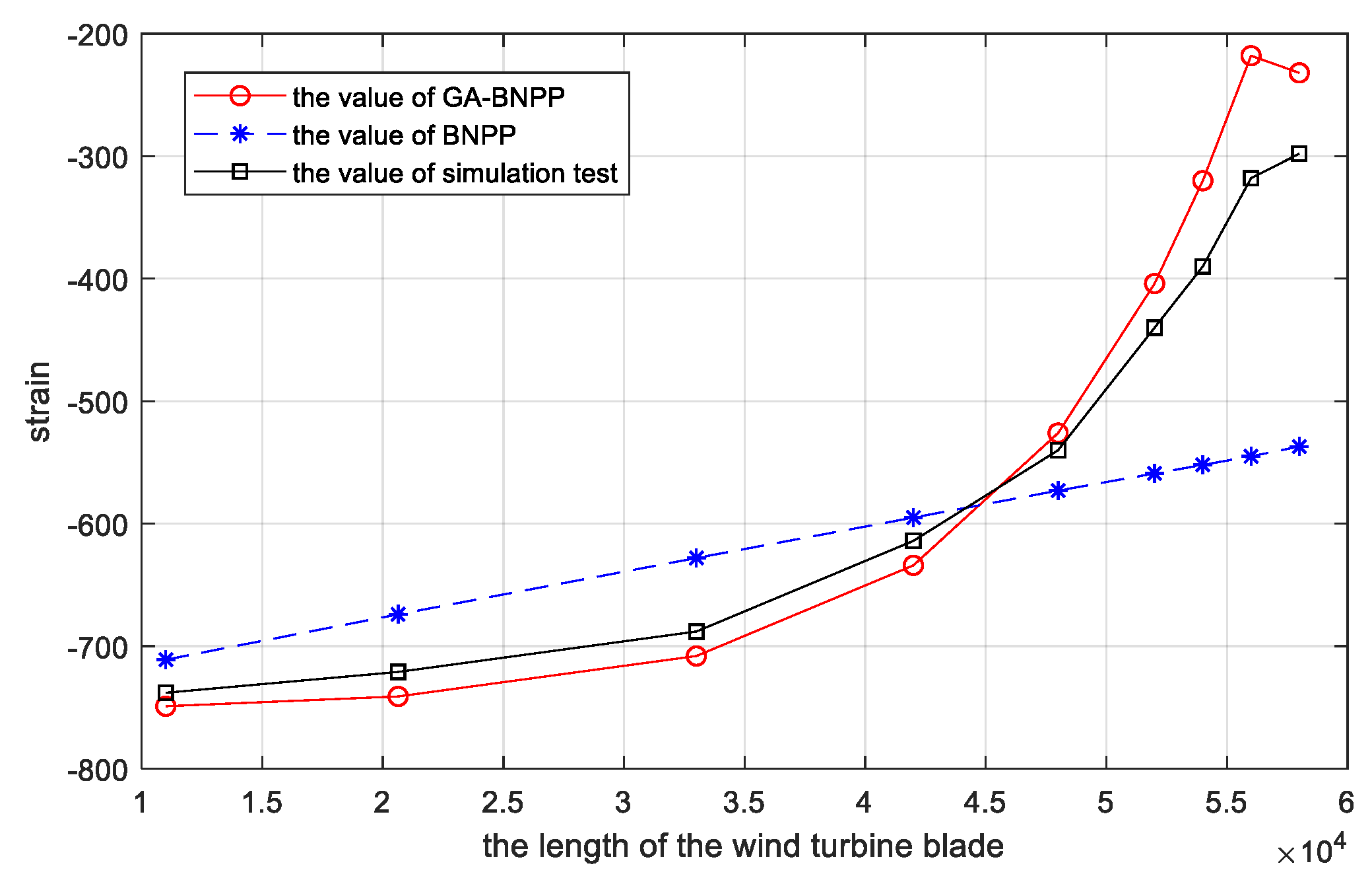
The unmeasured points on trailing edge at 33.00 m, 42.00 m, 48.00 m, 52.00 m, 54.00 m, 56.00 m, 58.00 m, 63.00 m, and 65.00 m from the root of the blade were chosen to predict their strain by using the BPNN. The contrast figures of BPNN, GA-BPNN, and the ANSYS simulation data are shown in Figure 11. The conclusion is the same as the analysis of the center of the suction side, both BPNN and GA-BPNN had a high accuracy to predict the strain, and the GA-BPNN had a smaller error. Thus, GA-BPNN is more suitable for the strain forecast of the full-scale static testing of wind turbine blades.

5. Conclusions

The calculation and prediction of blade strain in the full-scale static testing of wind turbine blades are very complex and difficult by traditional numerical methods, and the numbers of measuring points as well as strain gauges arranged on the blade are limited, so the test data have insufficient significance to the calibration of the blade design. As a result of these concerns, this paper proposed a strain prediction method for wind turbine blades using a GA-BPNN with applied loads, loading positions, and displacement as inputs, and tried to provide more data for the wind turbine blades’ health assessment and life prediction when the measurement points in full-scale static testing of wind turbine blades are limited:

(1)

Taking advantage of the neural network in dealing with complex problems, this paper established a strain–predictive GA-BPNN model for the center and the trailing edge of the suction side based on the full-scale static testing results of a certain wind turbine blade.

(2)

The GA-BPNN had a better performance on strain prediction in full-scale static testing of wind turbine blades than the BPNN. In the training process, the relevant regression coefficient trained by GA-BPNN was closer to 1 than the BPNN. In the test process, all the average errors of GA-BPNN were smaller than those of the BPNN. In the prediction process, the values analyzed by the GA-BPNN were closer to the theoretical values (simulation test values) than those analyzed by the BPNN.

(3)

The strain of unmeasured points at the center and the trailing edge of the suction side were predicted by strain–predictive BPNN model, respectively. For strain prediction of the points at the center of the suction side, the relative error rate of the test sample output was within 6.5%. While for strain prediction of the points at the trailing edge of the suction side, the relative error rate of the test sample output was within 18%. Compared with the prediction results of the center of suction side, the error of the trailing edge was relatively larger. For the trailing edge is the faying surface of suction side and pressure side, and the strain is influenced by more factors such as binder type, binder parameters, physical dimension, etc., thus, more inputs are needed to get a more accurate prediction.

(4)

The unmeasured points at 33.00 m, 42.00 m, 48.00 m, 52.00 m, 54.00 m, 56.00 m, 58.00 m, 63.00 m, and 65.00 m from the root of the blade were chosen to predict their strain using the BPNN. Comparing the prediction results with the ANSYS simulation data, both the BPNN and GA-BPNN had a high accuracy in predicting the strain, and the GA-BPNN had a smaller error. Thus, the GA-BPNN is more suitable for strain prediction of wind turbine blade static testing.

References

- Malhotra, P.; Hyers, R.W.; Manwell, J.F.; McGowan, J.G. A review and design study of blade testing systems for utility-scale wind turbines. Renew. Sustain. Energy Rev. 2012, 16, 284–292. [Google Scholar] [CrossRef]
- Fagan, E.M.; Flanagan, M.; Leen, S.B.; Flanagan, T.; Doyle, A.; Goggins, J. Physical experimental static testing and structural design optimization for a composite wind turbine blade. Compos. Struct. 2017, 16, 90–103. [Google Scholar] [CrossRef]
- Yang, T.; Du, W.C.; Yang, H.; Ma, C. Static load strain test of wind turbine blades. Res. Explor. Lab. 2011, 30, 33–36. [Google Scholar]
- Pan, Z.J.; Wu, J.Z. Effects of structure nonlinear on full-scale wind turbine blade static test. J. Tongji Univ. (Nat. Sci.) 2017, 45, 1491–1497. [Google Scholar]
- Zhu, S.P.; Yue, P.; Yu, Z.Y.; Wang, Q.Y. A combined high and low cycle fatigue model for life prediction of turbine blades. Materials 2017, 10, 698. [Google Scholar] [CrossRef] [PubMed]
- Liao, D.; Zhu, S.P.; Correia, J.A.F.O.; De Jesus, A.M.P.; Calçada, R. Computational framework for multiaxial fatigue life prediction of compressor discs considering notch effects. Eng. Fract. Mech. 2018, 202, 423–435. [Google Scholar] [CrossRef]
- Meng, D.; Yang, S.; Zhang, Y.; Zhu, S.P. Structural reliability analysis and uncertainties-based collaborative design and optimization of turbine blades using surrogate model. Fatigue Fract. Eng. Mater. Struct. 2018. [Google Scholar] [CrossRef]
- Zhu, S.P.; Liu, Q.; Peng, W.; Zhang, X.C. Computational-experimental approaches for fatigue reliability assessment of turbine bladed disks. Int. J. Mech. Sci. 2018, 142–143, 502–517. [Google Scholar] [CrossRef]
- Meng, D.; Liu, M.; Yang, S.; Zhang, H.; Ding, R. A fluid-structure analysis approach and its application in the uncertainty-based multidisciplinary design and optimization for blades. Adv. Mech. Eng. 2018, 10, 1–7. [Google Scholar] [CrossRef]
- Tarfaoui, M.; Nachtane, M.; Boudounit, H. Finite element analysis of composite offshore wind turbine blades under operating conditions. J. Therm. Sci. Eng. Appl. 2018. [Google Scholar] [CrossRef]
- Tarfaoui, M.; Shah, O.R.; Nachtane, M. Design and optimization of composite offshore wind turbine blades. J. Energy Resour. Technol. 2019, 141, 051204. [Google Scholar] [CrossRef]
- Tarfaoui, M.; Nachtane, M.; Khadimallah, H.; Saifaoui, D. Simulation of mechanical behavior and damage of a large composite wind turbine blade under critical loads. Appl. Compos. Mater. 2018, 25, 237–254. [Google Scholar] [CrossRef]
- Hu, W.; Choi, K.K.; Cho, H. Reliability-based design optimization of wind turbine blades for fatigue life under dynamic wind load uncertainty. Struct. Multidiscip. Optim. 2016, 54, 953–970. [Google Scholar] [CrossRef]
- Hu, W.; Choi, K.K.; Zhupanska, O.; Buchholz, J. Integrating variable wind load, aerodynamic, and structural analyses towards accurate fatigue life prediction in composite wind turbine blades. Struct. Multidiscip. Optim. 2016, 53, 375–394. [Google Scholar] [CrossRef]
- Yang, J.C.; Park, D.S. Fingerprint Verification Based on Invariant Moment Features and Nonlinear BPNN. Int. J. Control. Syst. 2008, 6, 800–808. [Google Scholar]
- Moghaddam, M.A.; Golmezergi, R.; Kolahan, F. Multi-variable measurements and optimization of GMAW parameters for API-X42 steel alloy using a hybrid BPNN–PSO approach. Measurement 2016, 92, 279–287. [Google Scholar] [CrossRef]
- Huang, Q.; Jiang, D.; Hong, L.; Ding, Y. Application of Wavelet Neural Networks on Vibration Fault Diagnosis for Wind Turbine Gearbox; Springer: Berlin/Heidelberg, Germany, 2008; Volume 5264, pp. 313–320. [Google Scholar]
- Chen, J.S.; Chen, W.G.; Li, J.; Sun, P. A generalized model for wind turbine faulty condition detection using combination prediction approach and information entropy. J. Environ. Inf. 2018, 32, 14–24. [Google Scholar] [CrossRef]
- Zhang, Y.; Zheng, H.; Liu, J.; Zhao, J.; Sun, P. An anomaly identification model for wind turbine state parameters. J. Clean. Prod. 2018, 195, 1214–1227. [Google Scholar] [CrossRef]
- Liu, T. The limit cycle oscillation of divergent instability control based on classical flutter of blade section. J. Vibro Eng. 2017, 19, 5114–5136. [Google Scholar] [CrossRef]
- Ding, S.; Su, C.; Yu, J. An optimizing BP neural network algorithm based on genetic algorithm. Artif. Intell. Rev. 2011, 36, 153–162. [Google Scholar] [CrossRef]
- Kuang, Y.; Singh, R.; Singh, S.; Singh, S.P. A novel macroeconomic forecasting model based on revised multimedia assisted BP neural network model and ant Colony algorithm. Multimed. Tools Appl. 2017, 76, 18749–18770. [Google Scholar] [CrossRef]
- Wang, W.; Li, M.; Hassanien, R.H.E.; Ji, M.E.; Feng, Z. Optimization of thermal performance of the parabolic trough solar collector systems based on GA-BP neural network model. Int. J. Green Energy 2017, 14, 819–830. [Google Scholar] [CrossRef]
- Xu, H.; Li, W.; Li, M.; Hu, C.; Zhang, S.; Wang, X. Multidisciplinary robust design optimization based on time-varying sensitivity analysis. J. Mech. Sci. Technol. 2018, 32, 1195–1207. [Google Scholar] [CrossRef]
- Zhou, W.H.; Xiong, S.Q. Optimization of BP Neural Network Classifier Using Genetic Algorithm; Springer: Berlin/Heidelberg, Germany, 2013. [Google Scholar]
- GB/T 25384-2010. Turbine Blade of Wind Turbine Generator Systems-Full-Scale Structural Test of Rotor Blades; Standards Press of China: Beijing, China, 2010. [Google Scholar]
Figure 1.
Back propagation neural network (BPNN) structure.
Figure 2.
Flow chart of genetic algorithm (GA)-BPNN.
Figure 3.
The structure of a wind turbine blade.
Figure 4.
The locations and positions of strain gauges on the wind turbine blade.
Figure 5.
Applied loading diagram of the full-scale static testing.
Figure 6.
(a) Regression curve of the BPNN model error; (b) regression curve of the GA-BPNN model error; (c) GA iteration curve graph of mean square error; (d) GA iteration curve graph of fitness function value. (e) The fitting results comparison of the training set about BPNN; (f) The fitting results comparison of the training set about GA-BPNN.
Figure 7.
The comparison results of prediction errors for the center of suction side.
Figure 8.
The comparison of GA-BPNN, BPNN, and the simulation test.
Figure 9.
(a) Regression curve of the BPNN model error; (b) regression curve of the GA-BPNN model error; (c) GA-iteration curve graph of mean square error; (d) GA-iteration curve graph of fitness function value. (e) The fitting results comparison of the training set about BPNN; (f) The fitting results comparison of the training set about GA-BPNN.
Figure 10.
The comparison results of prediction errors for the trailing edge.
Figure 11.
The comparison of BPNN, GA-BPNN, and the simulation test.