Early Fault Detection of Wind Turbines Based on Operational Condition Clustering and Optimized Deep Belief Network Modeling

Abstract

Health monitoring and early fault detection of wind turbines have attracted considerable attention due to the benefits of improving reliability and reducing the operation and maintenance costs of the turbine. However, dynamic and constantly changing operating conditions of wind turbines still pose great challenges to effective and reliable fault detection. Most existing health monitoring approaches mainly focus on one single operating condition, so these methods cannot assess the health status of turbines accurately, leading to unsatisfactory detection performance. To this end, this paper proposes a novel general health monitoring framework for wind turbines based on supervisory control and data acquisition (SCADA) data. A key feature of the proposed framework is that it first partitions the turbine operation into multiple sub-operation conditions by the clustering approach and then builds a normal turbine behavior model for each sub-operation condition. For normal behavior modeling, an optimized deep belief network is proposed. This optimized modeling method can capture the sophisticated nonlinear correlations among different monitoring variables, which is helpful to enhance the prediction performance. A case study of main bearing fault detection using real SCADA data is used to validate the proposed approach, which demonstrates its effectiveness and advantages.

1. Introduction

With increasing global energy demand, wind energy as a promising clean source of renewable energy has become an indispensable force in solving world energy problems. The latest annual report released by the Global Wind Energy Council (GWEC) [1] shows that the cumulative and new installed capacity in the world had reached 539,123 MW and 52,492 MW, respectively, by the end of 2017. However, wind turbines are generally situated in remote locations and have harsh operating environments, resulting in frequent failures and undesired shutdowns. High maintenance costs and downtime losses seriously affect the economic benefits of wind farms and also have a powerful impact on the healthy development of the wind power industry [2]. There is an urgent need for effective prognostics and health management (PHM) technologies to address these problems. In particular, fault detection is a premise for PHM. Therefore, it is crucial and valuable to develop advanced health monitoring and fault detection methods to detect impending wind turbine faults as early as possible in order to avoid secondary damage and even catastrophic accidents.

Vibration analysis and oil monitoring have become two commonly used techniques for wind turbine condition monitoring [3,4,5,6]. However, both techniques are sophisticated and expensive in their practical application, since additional investments, including installing extra sensors and data acquisition devices, are required. Alternatively, supervisory control and data acquisition (SCADA) systems, which have been widely installed in large-scale wind turbines, can collect and record the operational state information from wind turbines and their critical components on a regular basis [7]. Compared with the vibration and oil monitoring methods, SCADA-based monitoring has been considered to be cost-effective due to the availability of a large amount of monitoring data and no additional cost. As a result, SCADA-based wind turbine health monitoring has attracted wide attention in recent years [8], and different SCADA data analysis methods have been proposed.

Zaher et al. [9] developed normal behavior models for gearboxes and generators based on artificial neural networks by analyzing SCADA data. The case study results demonstrated that it was possible to detect faults as early as 6 months and 16 months before final replacement of the gearbox and generator, respectively. Guo et al. [10] employed a nonlinear state estimation method to construct a normal behavior model of generator temperature using 2 min and 10 min averaged SCADA data. A real case study showed that the method was able to predict generator faults about 8.5 h before the actual failure. Kusiak et al. [11] introduced a neural network to model the normal behavior of generator bearings by using 10 s SCADA data. The research showed that the method could identify anomalies about 1.5 h ahead of the eventual failure. Schlechtingen et al. [12,13] proposed an adaptive neuro-fuzzy inference system combining artificial neural network and fuzzy logic analysis and constructed 45 normal behavior models using 10 min averaged SCADA data. Case studies illustrated that the system could detect the potential failures of wind turbines months in advance and provide the root causes of these failures based on simple if–then rules. Bangalore et al. [14,15] applied artificial neural networks to establish normal behavior models of gearboxes. Case studies with 10 min averaged SCADA data showed that the proposed methods were able to detect gearbox anomalies ahead of the condition monitoring system. Bi et al. [16] presented a pitch fault detection procedure using a normal behavior model based on the performance curve and carried out six case studies. The results illustrated that the proposed method could detect pitch faults earlier than the artificial intelligence approaches investigated. Different methods have been used to model the normal behavior of wind turbines. Further, residuals between the predicted values of the models and actual measured values of the expected output variable were used to identify the anomalies of wind turbines. Practically, wind turbine operating conditions are complicated and changeable and present multiple operation regions due to varying external wind speed and a complex internal control scheme, which poses great challenges for effective and reliable fault detection. However, most existing monitoring approaches only focus on a single whole operating condition, so they cannot fully consider the dynamic operating characteristics of wind turbines, leading to unsatisfactory detection performance, such as high rates of false alarms or missed detections. On the other hand, conventional health monitoring methods, such as neural networks, naturally have classical shallow structures, which poses a difficulty in effectively capturing sophisticated nonlinear relationships among monitoring variables.

To address the above issues, a novel general health monitoring approach for wind turbines under varying operating conditions is proposed in this paper. This approach is data-driven and based on monitoring data collected from wind turbine SCADA systems. First, to consider the dynamic behavior and multiple operating characteristics of wind turbines, an operation condition partition scheme using a clustering algorithm is proposed to partition the whole operation into multiple sub-operation conditions. This is a divide-and-conquer strategy and can enable the building of local monitoring models in different sub-operation conditions, which can improve the reliability and accuracy of fault detection compared to a global monitoring model. Second, to overcome the shortcoming of traditional shallow structure–based methods, a deep learning–based modeling approach is proposed to deal with relevant SCADA data to capture the sophisticated nonlinear correlations among monitoring variables. In recent years, motivated by the powerful ability of feature learning and nonlinear modeling of deep learning methods, convolutional neural network [17], autoencoder [18], denoising autoencoder [19], and multilayered extreme learning machines [20] have been used in many classification and regression tasks. Specifically, deep belief networks (DBNs) [21], a typical class of deep learning methods, are used in this study, which are naturally probabilistic generative models with multilayered architecture. Compared with shallow neural network methods, DBNs can capture complex nonlinear features, have a powerful modeling capacity and are quite suitable for modeling complex SCADA data [22]. DBNs have received attention in the fields of wind speed prediction [23], mechanical engineering fault diagnosis [24] and complex system fault detection [25]. The performance of DBNs is largely dependent on their structural parameters. However, there is no uniform rule for parameter selection. Various optimization algorithms have shown the ability to deal with complex problems, such as particle swarm [26] and genetic algorithm [27]. In particular, chicken swarm optimization (CSO), a novel bionic heuristic optimization algorithm, is introduced for optimizing model parameters of DBNs. In summary, the main contributions of this paper are as follows:

(1)

A general multioperation condition partition scheme is proposed to partition normal state data into several different clusters. Then, normal behaviors are built under different condition clusters. This divide-and-conquer strategy can help reduce false alarms caused by methods that only consider a single operating condition.

(2)

An optimized DBN (ODBN) model with CSO is designed to capture the normal behavior in each cluster, which reduces the complexity of parameter selection of DBNs. To the best of our knowledge, it is the first time DBN is applied to deal with complex SCADA data from wind turbines for the purpose of fault detection.

(3)

A real case from wind turbine main bearing fault was used to evaluate the performance of the proposed health monitoring approach using the SCADA data of multiple wind turbines from a real wind farm, and comparative studies were conducted.

The remainder of this paper is organized as follows. Section 2 describes the multioperation condition problem and the operation parameters studied in this paper. In Section 3, the proposed health monitoring framework is presented, the steps are explained, and the presented methodologies are described in detail. Section 4 presents the case study and discussion, and results are compared and analyzed. Conclusions are summarized in Section 5.

2. Problem Description

As critical equipment for wind power generation, a wind turbine is typically a complex electromechanical system composed of a variety of components and subsystems, including gearbox, generator, shaft, bearing, and power electronics, among many others [28]. In practical applications, wind turbines are generally located in remote areas and perennially operate under adverse weather conditions, such as storms, dust, and extreme temperature differentials. In addition, they are also affected by mechanical, electrical, and control strategies. These kinds of situations lead to operating conditions characterized by complexity and variability. As discussed in the first section, one of the primary disadvantages of existing data-driven condition monitoring approaches for wind turbines is that they only take into account a single operating condition, ignoring the characteristics that exist in the process of operating wind turbines. Due to their highly dynamic operating conditions, variations in the abnormal states of turbines are always easily masked by the condition fluctuations, making it difficult to accurately assess the health status and thereby causing frequent false alarms. In this case, it is highly desirable to develop reliable health monitoring approaches to deal with the dynamic and varying operating conditions of wind turbines.

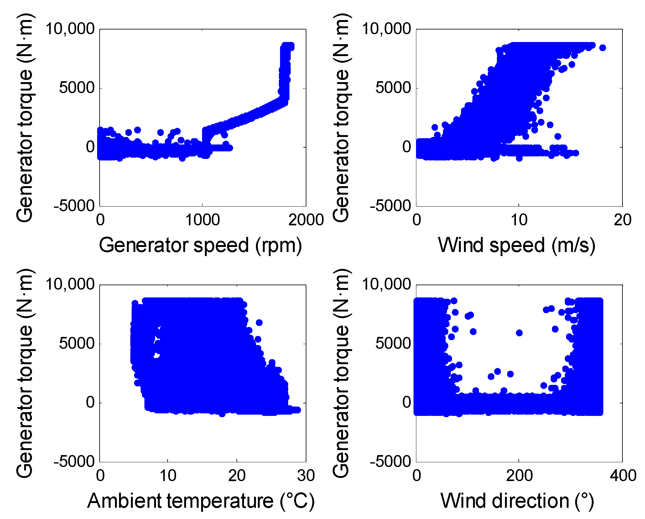
Wind turbine SCADA data contain hundreds of monitoring parameters related to the health of the wind turbine and its critical components. Typically, these parameters include wind conditions (e.g., wind speed, wind direction), power output, blade pitch angle, generator torque and speed, temperatures (e.g., main bearing temperature, gearbox oil temperature, nacelle temperature, and ambient temperature) among others [29]. Several parameters are closely related to the wind turbine operating conditions, which can be referred to as operation parameters, describing the external and internal changes of the turbine operation due to constantly changing wind speed and complex switched control schemes. Typically, these primarily include environmental parameters such as wind speed, wind direction, and ambient temperature, and control parameters such as generator speed and torque [30]. To facilitate the understanding of the operating characteristics of the wind turbine, historical SCADA operation data were collected from a 1.5 MW turbine under normal operation from July to August 2014, shown in Figure 1. Obviously, these operation parameters segment the wind turbine operating conditions into different operation regions to varying degrees, which truly reflects the multiple operating characteristics of the wind turbine. In this case, a global health monitoring model cannot describe the turbine behavior accurately and even fails to produce reliable detection results. Therefore, it is of great practical value to investigate efficient and reliable health monitoring methods, considering varying operating conditions in order to improve the accuracy of fault prediction and reduce operation and maintenance costs.

3. Proposed Health Monitoring Framework

In this study, a novel health monitoring framework for wind turbines under varying operating conditions is proposed, and its flowchart is shown in Figure 2. It is general and can be used for fault detection of different wind turbine subsystems and components. The main idea of the proposed framework is to build normal behavior models relying on only historical normal SCADA data from wind turbines and then perform fault detection based on the evaluation results of residuals between the predicted values and actual measured values. The changes of the residuals will give an indication of possible faults. Usually, normal test samples will produce a low residual value since they can well satisfy the learned normal model, whereas faulty test samples will produce high residual values and therefore be identified as faults. Generally, the proposed framework mainly consists of four sequential parts: operation condition partition, variable selection, model development and anomaly detection. The detailed procedures are summarized as follows:

(1)

Collect normal SCADA data from multiple wind turbines on a wind farm.

(2)

Choose operation parameters that characterize the complex operating conditions of wind turbines and segment the operation parameter data into K clusters using the k-means method and silhouette index. The obtained K clusters represent the corresponding K operating conditions, i.e., $[C_1, C_2, \cdots , C_K]$. Then, divide the normal state data into corresponding K parts based on the partitioned operating conditions.

(3)

Select appropriate modeling variables for each operating condition by combining three variable selection techniques, and the final selected variables for different operating clusters can be represented as $[V_1, V_2, \cdots , V_K]$.

(4)

Build a normal behavior model under each operating condition using ODBNs to explore the sophisticated nonlinear characteristics among modeling variables, resulting in multiple DBN models, denoted as ${[\mathrm{DBN}}_1,{ \mathrm{DBN}}_2, \cdots ,{ \mathrm{DBN}}_K]$ for K operating clusters.

(5)

Calculate the threshold for abnormal detection under different operating conditions using the Mahalanobis distance (MD) measure to automatically identify the anomalies that occur in the operation of the wind turbines, i.e., $[{\mathrm{MD}}_1,{ \mathrm{MD}}_2, \cdots ,{ \mathrm{MD}}_K]$.

(6)

For the new incoming SCADA data, first recognize the operating condition $C_i$ that it belongs to, then select the corresponding modeling input variable $V_i$ and predict the output using the constructed DBN_i. Next, compute the MD value and compare it with the threshold MD_i under condition $C_i$, and then output the real-time online health monitoring results.

3.1. Data Preprocessing

It should be noted that data preprocessing is a necessary step in wind turbine condition monitoring prior to modeling using SCADA data [7]. During the long-time continuous operation of a wind turbine, a large number of outliers and invalid values may be generated and included in the SCADA data because of sensor failures, communication errors, or other issues. These outliers and invalid values will directly impact the performance of the model to be trained, and they should be removed first. To reduce the effects of noise and randomness contained in SCADA data, all data are smoothed prior to selecting modeling variables. Additionally, considering that different operation parameters often have different value ranges, it is a common step to normalize the initial operation data before partitioning the conditions to ensure that each operation variable lies within the specified range between 0 and 1. Specifically, in this study, this step can be simply realized by using the following equation [31]:

$$Y_{ij}=\frac{x_{ij}-\min (x_j)}{\max (x_j)-\min (x_j)},$$

(1)

where $x_{ij}$ is the $i\mathrm{th}$ value of variable $j$, and $\min (x_j)$ and $\max (x_j)$ are the minimum and maximum values of variable $j$, respectively.

3.2. Operation Condition Partition Using K-Means Clustering

The reasonable selection of wind turbine operation parameters is a prerequisite to realize the partition of operating conditions. As mentioned in Section 2, for a wind turbine, the operation parameters mainly include the following five variables: wind speed, wind direction, ambient temperature, generator speed, and generator torque, which are closely related to the operating conditions. Generally, the operating conditions can be partitioned into several typical operation regions depending on the above operation parameters. As an unsupervised learning method, k-means clustering [32] has become one of the most prevalent and widely used partitioning clustering algorithms due to its advantages of usability, efficiency, simplicity and successful experience [33]. Hence, in this study, this method is adopted for the condition partition. Certainly, other clustering methods can also be considered. The aim of k-means is to allocate all data samples into K clusters by minimizing the sum of the squared error over all K clusters, denoted as follows [33]:

$$J=\underset{O}{\arg \min }{\displaystyle \sum _{i=1}^K{\displaystyle \sum _{x_j\in O_i}{‖x_j-{\mu }_i‖}^2}},$$

(2)

where $O=\{O_1, O_2, \dots , O_K\}$ is the set of K clusters, ${\mu }_i$ is the cluster centroid of the $i\mathrm{th}$ cluster, $\{x_1, x_2, \dots , x_N\}$ is the cluster samples, and $N$ is the number of samples.

In the k-means algorithm, the number of clusters K is a key parameter. Silhouette [34] is one of the indices for evaluating the clustering number by combining the two factors of cohesion and resolution, which is employed to determine K in this paper. The silhouette value for the $i\mathrm{th}$ point, $S(i)$, is expressed as

$$S(i)=\frac{b\left(i)-a\right(i)}{\max \{a\left(i), b\right(i\left)\right\}}, i=1, 2, \dots , N,$$

(3)

where $a(i)$ represents the average distance from the $i\mathrm{th}$ point to the other points in the same cluster and $b(i)$ denotes the minimum average distance from the point to points in a different cluster. The range of $S(i)$ is [–1, 1]. A higher value of $S(i)$ indicates that the $i\mathrm{th}$ point is clustered more properly. The average of all $S(i)$ is then the final silhouette value for a given cluster number.

3.3. Variable Selection

To construct the normal behavior model, it is necessary to first determine the modeling variables in each operating condition. Usually, there are multiple types of relationship among the variables and various techniques can be applied to assess each type of relationship [35]. Three typical variable selection techniques are proposed in [36,37,38], the Pearson, Spearman, and Kendall correlation coefficients, which are statistics for measuring the linearity, monotonicity, and dependence among variables, respectively. This paper combines the three technologies to select the input variables most relevant to the output variables. It is worth noting that the computation results of these three methods are all in the range of –1 to 1, and a higher absolute value indicates a stronger correlation between the input and output.

3.4. Proposed ODBN Method

The use of wind turbine SCADA systems becomes the primary option for most wind farms, and as a result, large amounts of monitoring data can be acquired and archived regularly. The measured SCADA data have notable features of complex nonlinearity and strong coupling due to the interdependence and interaction between the different subsystems of the wind turbines during operation. Consequently, in this section, ODBNs are proposed to capture the latent nonlinear correlations in the SCADA monitoring data, and the details are described as follows.

3.4.1. DBN Architecture

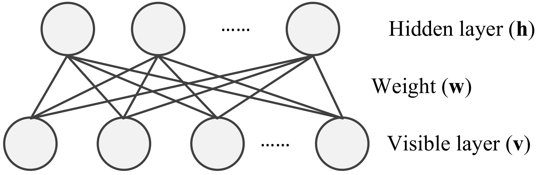
The structure of DBNs comprises probabilistic generative models composed of multiple stacked restricted Boltzmann machines (RBMs). As displayed in Figure 3, each RBM is a kind of two-layer stochastic neural network consisting of one visible layer and one hidden layer. There are connection weights between the visible layer and the hidden layer, while the units in each layer are restricted to each other.

Assuming that the RBM is a Bernoulli–Bernoulli model (BB-RBM), for a given set of states $(v, h)$, the energy function is defined as

$$E(v, h; \theta )=-{\displaystyle \sum _{i=1}^V{\displaystyle \sum _{j=1}^H{\omega }_{ij}{v}_i{h}_j}}-{\displaystyle \sum _{i=1}^V{b}_i{v}_i}-{\displaystyle \sum _{j=1}^H{a}_j{h}_j},$$

(4)

where $\theta =\{w, a, b\}$ denotes the model parameters; $v_i$ and $h_j$ are the visible unit $i$ and the hidden unit $j$, respectively; ${\omega }_{ij}$ is the connection weight between $i$ and $j$; $b_i$ and $a_j$ are the biases of $v_i$ and $h_j$; and $V$ and $H$ are the number of visible and hidden units, respectively. Given the energy function, the joint probability over the visible and hidden units can be described as follows:

$$p(v, h; \theta )=\frac{1}{Z}\exp (-E(v, h; \theta )),$$

(5)

where $Z={\displaystyle \sum _v{\displaystyle \sum _h\exp (-E(v, h; \theta ))}}$ is the partition function.

Since the visible–visible and hidden–hidden units are not connected, the probabilities of the visible unit $v_i$ and the hidden unit $h_j$ are independent. Therefore, the conditional distributions can be expressed as

$$p(h_j=1\left|v; \theta \right.)=\delta ({\displaystyle \sum _{i=1}^V{\omega }_{ij}{v}_i}+a_j),$$

(6)

$$p(v_i=1\left|h; \theta \right.)=\delta ({\displaystyle \sum _{j=1}^H{\omega }_{ij}{h}_j}+b_i),$$

(7)

where $\delta (x)=1/(1+exp(x))$ represents the logistic sigmoid function. The model parameters $\theta$ of the RBM can be obtained by a contrastive divergence method [39]. The update rule for the weight $w$ is written as follows:

$$\Delta {\omega }_{ij}= \epsilon \left(\langle v_i{h}_j\rangle {}_{data} - \langle v_i{h}_j\rangle {}_k\right),$$

(8)

where $\epsilon$ refers to the learning rate, ${\langle \cdot \rangle }_{data}$ denotes the expectation of the training data, and ${\langle \cdot \rangle }_k$ represents the expectation of the sample distribution after k-step Gibbs sampling. A more detailed description of the training process of the RBM can be seen in [40].

The general architecture of a DBN model with n hidden layers is shown in Figure 4. The bottom layer of the DBN accepts input data and then passes the data to hidden layers to complete the learning process. To handle real-valued data, a Gaussian–Bernoulli RBM (GB-RBM) should be adopted in the first RBM model, and BB-RBM is applied in the rest of the RBM models. The learning process of the DBN consists of two phases, pretraining and fine-tuning. Pretraining is the process of initializing the connection weights and biases of the network in a greedy layer-wise unsupervised manner. In this phase, each RBM is trained from bottom to top individually. In the fine-tuning phase, the parameters of the DBN model are updated with the back-propagation algorithm in a supervised fashion. Thus, DBNs realize the organic combination of unsupervised and supervised learning, which can effectively improve the modeling capacity. In this study, a four-layer DBN, including the bottom input layer, the top output layer, and two hidden layers, are used for SCADA data modeling.

3.4.2. ODBN Method

It is worth noting that although DBNs can enhance the performance of prediction to some extent, the performance is highly influenced by their structural parameters. Therefore, how to determine and achieve optimal model parameters has become a primary challenge for DBNs. The main parameters of concern in this paper are the number of neurons in the two hidden layers of the DBN. In general, these parameters can be obtained experimentally, but it is time-consuming and laborious. CSO is a novel bionic heuristic optimization algorithm that mimics the hierarchy in the chicken swarm and the food search behavior [41]. The optimization algorithm obtains the optimal parameters by dividing the chicken swarm into several subgroups and competing among different subgroups. Therefore, this algorithm is used for the adaptive optimization of the model parameters. The position of each individual in the chicken swarm represents a potential solution to the optimization problem. There are three types of chickens in the CSO: roosters, hens, and chicks. To search for the optimal solution in the search space, it is necessary to update the position of each type of chicken. The position update equation for the roosters is depicted as follows:

$$x_{i,j}^{t+1}=x_{i,j}^t\cdot (1+\mathrm{Randn}(0,{\sigma }^2)),$$

(9)

$${\sigma }^2=\left\{\begin{array}{l}1,\hspace{1em}\hspace{1em}\hspace{1em}\hspace{1em}\hspace{1em}\mathrm{if} f_i\le f_k\\ \exp (\frac{(f_k-f_i)}{\left|f_i\right|+\epsilon }),\hspace{1em}otherwise\end{array}\right.,$$

(10)

where t is the number of iterations; $\mathrm{Randn}(0,{\sigma }^2)$ is a Gaussian distribution with mean 0 and standard deviation ${\sigma }^2$; $i, k\in [1, r\mathrm{size}]$ and $i\ne k$, $r\mathrm{size}$ represent the number of roosters; $f_k$ and $f_i$ are the fitness values of rooster particles $i$ and $k$, respectively; and $\epsilon$ is a constant that is small enough. The position update equation for hens is as follows:

$$x_{i,j}^{t+1}=x_{i,j}^t+S1\cdot \mathrm{Rand}\cdot (x_{r1,j}^t-x_{i,j}^t)+S2\cdot \mathrm{Rand}\cdot (x_{r2,j}^t-x_{i,j}^t),$$

(11)

$$S1=\exp (\frac{(f_i-f_{r1})}{\left|f_i\right|+\epsilon }),$$

(12)

$$S2=\exp (f_{r2}-f_i),$$

(13)

where $\mathrm{Rand}$ is a uniform number over [0,1]; $r_1$ is an index of the rooster, which is the $i\mathrm{th}$ hen’s group mate; and $r_2$ is a randomly chosen index of a chicken (rooster or hen) from the swarm, and $r_1\ne r_2$. The position update equation for chicks is as follows:

$$x_{i,j}^{t+1}=x_{i,j}^t+FL\cdot (x_{m,j}^t-x_{i,j}^t),$$

(14)

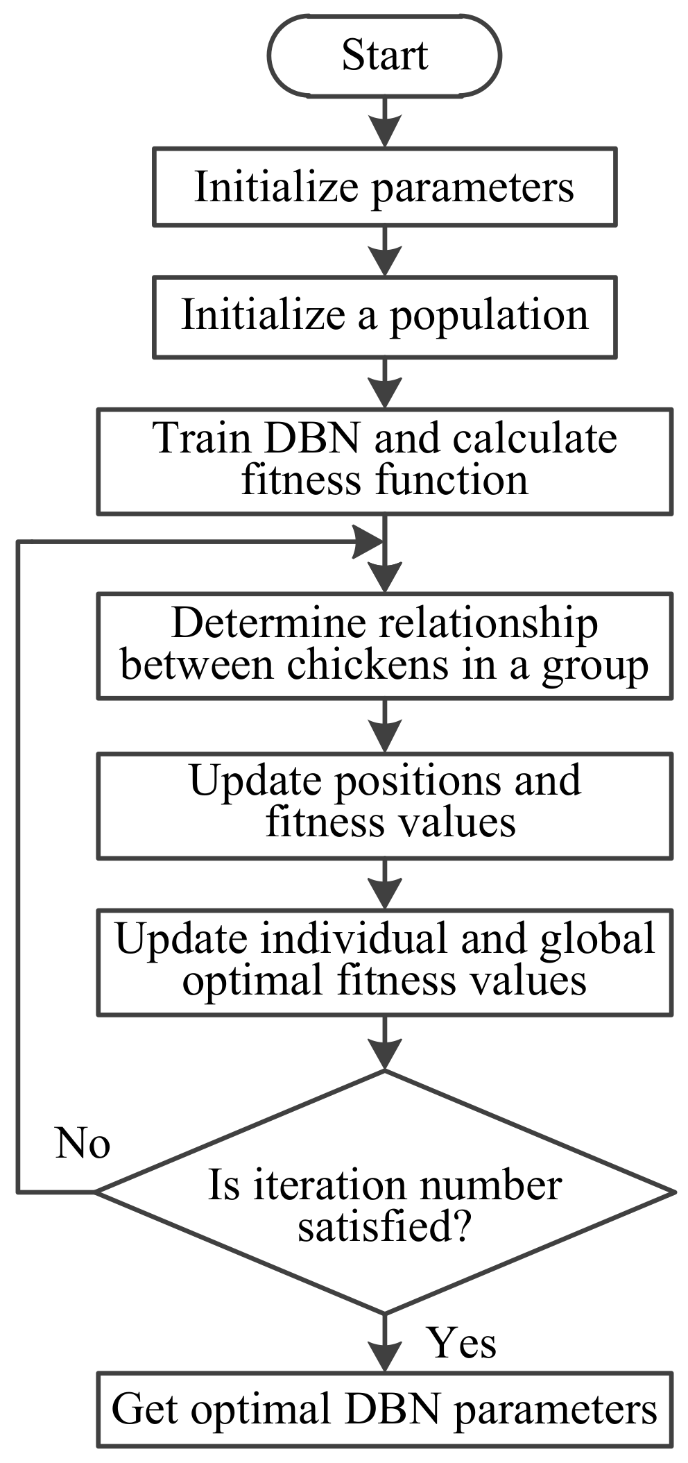
where $FL$ refers to a parameter that means the chick would follow its mother to forage for food, and the range is [0, 2]; and $x_{m,j}^t$ is the position of the $i\mathrm{th}$ chick’s mother. In this paper, the position of each individual represents the number of neurons in the two hidden layers of the DBN. Figure 5 gives the flowchart of ODBN with CSO, and the detailed procedure is explained as follows:

(1)

Initialize the parameters, including number of chickens, dimensions of individual positions, maximum iteration number, updated frequency of chicken swarm, and proportions of roosters, hens, and mother hens.

(2)

Randomly produce an initial population of chickens. Train the DBN and compute the fitness values, and determine the optimal individual and global fitness values and corresponding positions. Here, the root mean square error (RMSE) of the validation set is considered as the fitness function.

(3)

In the next iteration, first determine the relationship between the roosters, hens, and chicks in a group, and then update their positions according to Equations (9)–(14) and calculate their fitness values. Next, update the optimal individual and global fitness values and their corresponding positions.

Repeat step 3 until the maximum iteration number is reached and output the optimal parameters of the DBN. Note that the original CSO is a method for optimizing continuous values. Since the number of neurons in hidden layers of the DBN is an integer, the CSO that optimizes the continuous values is not applicable. Hence, when initializing the population of chickens and updating the positions of roosters, hens, and chicks, discretize them to meet the requirements.

3.5. Anomaly Detection Approach

The purpose of establishing ODBN normal behavior models is to continuously monitor the working status of the components being modeled and identify impending faults in a timely manner, which is important to avoid major faults of components and ensure the secure and stable operation of wind turbines. In this paper, an advanced health monitoring approach called MD is utilized for operational state monitoring and abnormal behavior identification. MD has been successfully adopted in the detection of abnormalities of wind turbines [14,15].

MD is a unitless distance measurement that can capture the correlation of variables in a process or system and is defined as follows:

$$M{D}_i=\sqrt{(X_i-\mu )C^{-1}{(X_i-\mu )}^T}, i=1, 2, \dots , n,$$

(15)

where $X_i=[X_{i1}, X_{i2}, \dots , X_{im}]$ is the $i\mathrm{th}$ observation vector, $n$ is the number of observations, $m$ is the total number of parameters, $\mu =[{\mu }_1, {\mu }_2, \dots , {\mu }_m]$ is the vector of mean values, $C$ is the covariance matrix, and $M{D}_i$ is the MD value for the $i\mathrm{th}$ vector $X_i$.

For health monitoring, the MD values for the validation set are used to calculate the threshold for anomaly detection. During the validation stage, wind turbines are in normal operation and no abnormal behavior occurs. The MD for the validation set can be expressed as follows:

$$M{D}_{refi}=\sqrt{(X_{refi}-{\mu }_{ref})C_{ref}^{-1}{(X_{refi}-{\mu }_{ref})}^{\mathrm{T}}},$$

(16)

where $X_{refi}=[V{E}_i, T{V}_i]$ represents the $i\mathrm{th}$ vector; $T{V}_i$ denotes the $i\mathrm{th}$ target value during the validation stage and $V{E}_i$ is the corresponding validation error; ${\mu }_{ref}$ and $C_{ref}$ are the mean value vector and the covariance matrix of $X_{ref}$, respectively. $M{D}_{refi}$ refers to the MD value for the $i\mathrm{th}$ vector $X_{refi}$.

After obtaining the healthy MD values in the validation stage, the anomaly detection threshold can be determined by fitting a two-parameter Weibull probability distribution function on these MD values [42]. The two-parameter Weibull distribution is described as

$$f(t)=\beta {\eta }^{-\beta }{(t)}^{\beta -1}{e}^{-{(\frac{t}{\eta })}^{\beta }},$$

(17)

where $\beta$ denotes the shape parameter and $\eta$ stands for the scale parameter.

The MD during the condition monitoring stage is depicted as follows:

$$M{D}_{newi}=\sqrt{(X_{newi}-{\mu }_{ref})C_{ref}^{-1}{(X_{newi}-{\mu }_{ref})}^{\mathrm{T}}},$$

(18)

where $X_{newi}=[P{E}_i, M{V}_i]$, $M{V}_i$ is the $i\mathrm{th}$ actual measured value from the SCADA system during the condition monitoring stage, and $P{E}_i$ is the model prediction error.

In this study, in order to reduce the false alarm rate, the MD value from the condition monitoring stage is identified as an anomaly if $f(M{D}_{newi})$ is less than 0.1%. At this point, an alarm signal is triggered to alert the operators about the operational states of the turbine so they can take appropriate action to avoid major faults.

4. Case Study and Discussion

In this section, a real case for main bearings is investigated to demonstrate the feasibility of the proposed approach in practical applications of wind turbine health monitoring, and the results obtained in each part are presented in detail.

4.1. Data Description

The SCADA data used in this paper are from a wind farm located in Inner Mongolia, China. All wind turbines in the wind farm are variable speed constant frequency with a rated power of 1.5 MW. The sampling interval of the SCADA data is 30 s. Each record includes a total of 25 discrete pieces of information, such as turbine state, time stamp, yaw state, etc. At the same time, 49 continuous parameters are also recorded, listed in

Table 1. Continuous parameters in SCADA data.

Continuous Parameter
Gearbox oil temperature	Wind direction	Current phase C	Absolute wind direction
Gearbox front bearing temperature	Generator speed	Converter side speed	Blade 1 motor current
Gearbox inlet oil temperature	Gearbox speed 1	Converter side torque	Blade 2 motor current
Generator front bearing temperature	Wind speed 1	Wind speed 1 s average	Blade 3 motor current
Generator rear bearing temperature	Wind speed 2	Wind speed 1 min average	Blade 1 motor temperature
Generator stator winding temperature	Active power	Wind speed 10 min average	Blade 2 motor temperature
Converter ambient temperature	Reactive power	Ambient temperature	Blade 3 motor temperature
Gearbox rear bearing temperature	Wind speed	Main bearing temperature	Hub temperature
Wind direction 1 s average	Voltage phase A	Nacelle temperature	Cable winding angle
Wind direction 1 min average	Voltage phase B	Active power 1 s average	Generator torque
Wind direction 10 min average	Voltage phase C	Active power 1 min average
Gearbox oil pump pressure	Current phase A	Active power 10 min average
Gearbox inlet oil pressure	Current phase B	Hydraulic system pressure

. The SCADA data for the majority of the turbines were available during the period from 1 July to 23 September 2014. In this paper, the SCADA data from 13 available turbines during the period 1 July to 31 August 2014 are investigated. Detailed descriptions of the datasets are listed in

Table 2. Description of SCADA datasets.

Dataset	Time Stamps	Turbines Considered
Modeling	1/7/2014–31/8/2014	6, 17, 24, 33–34, 37, 49, 53, 88
Testing normal behavior	30/7/2014–2/8/2014	20
	14/8/2014–17/8/2014	46
Testing abnormal behavior	10/9/2014–14/9/2014	42
	2/7/2014–4/7/2014	13

.

To obtain a reliable health monitoring model of the main bearing, it is necessary to include as much data as possible to cover all normal operation regions of the turbine. Therefore, Turbines 6, 17, 24, 33–34, 37, 49, 53, 88 were randomly selected for modeling. During the period from 1 July to 31 August 2014, there were no main bearing faults in these 9 turbines, which are suitable for establishing the normal behavior model of the main bearing. The number of samples of normal SCADA data from the nine turbines in normal operation during this period is 353,131.

Similarly, Turbines 20 and 46 did not experience main bearing faults, so are used to test the performance of the normal behavior of wind turbines. Whereas Turbines 42 and 13 experienced main bearing over temperature faults, so are employed to detect the abnormal behavior of the main bearing.

4.2. Model Development

In this section, the proposed health monitoring model for wind turbine main bearings is developed in detail based on the above methods. To investigate the prediction performance of the proposed modeling method in different operating conditions, the traditional algorithms are used for comparison. Several methods are also compared without considering the operating characteristics of wind turbines.

4.2.1. Operation Condition Partition

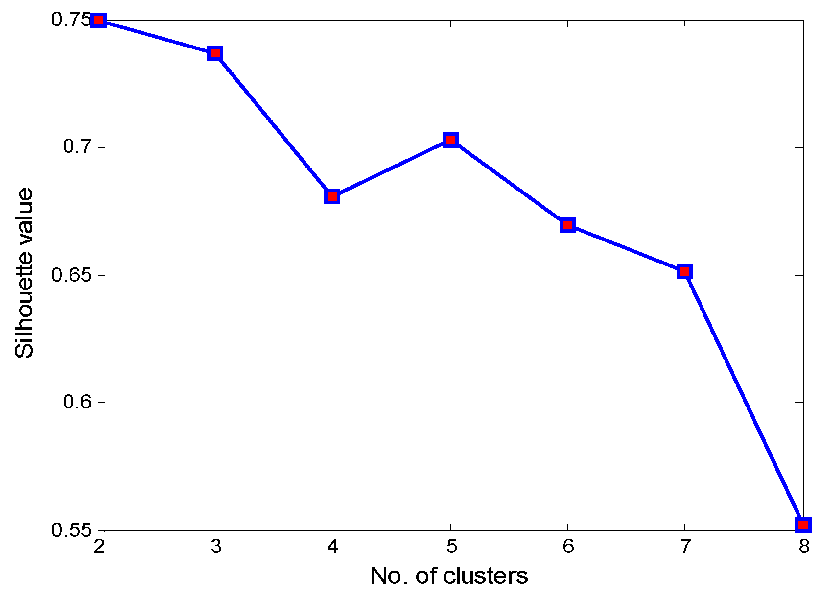
For the SCADA data from nine turbines in normal operation from 1 July to 31 August 2014, described in Section 4.1, the operation parameters representing the wind turbine operating conditions should first be extracted. Normally, the normalization of operation data is a basic step before partitioning the operating condition depending on the operation parameters to ensure the reliability of the clustering results. In this paper, in order to be more consistent with the operating characteristics of wind turbines, the number of clusters is set from two to eight, and the calculation results of the silhouette values are shown in Figure 6. From Figure 6, it can be seen that when the number of clusters is two, the silhouette value reaches the maximum value of 0.75. This result indicates that it is optimal to segment the wind turbine operating conditions into two sub-conditions, condition 1 (C₁) and condition 2 (C₂).

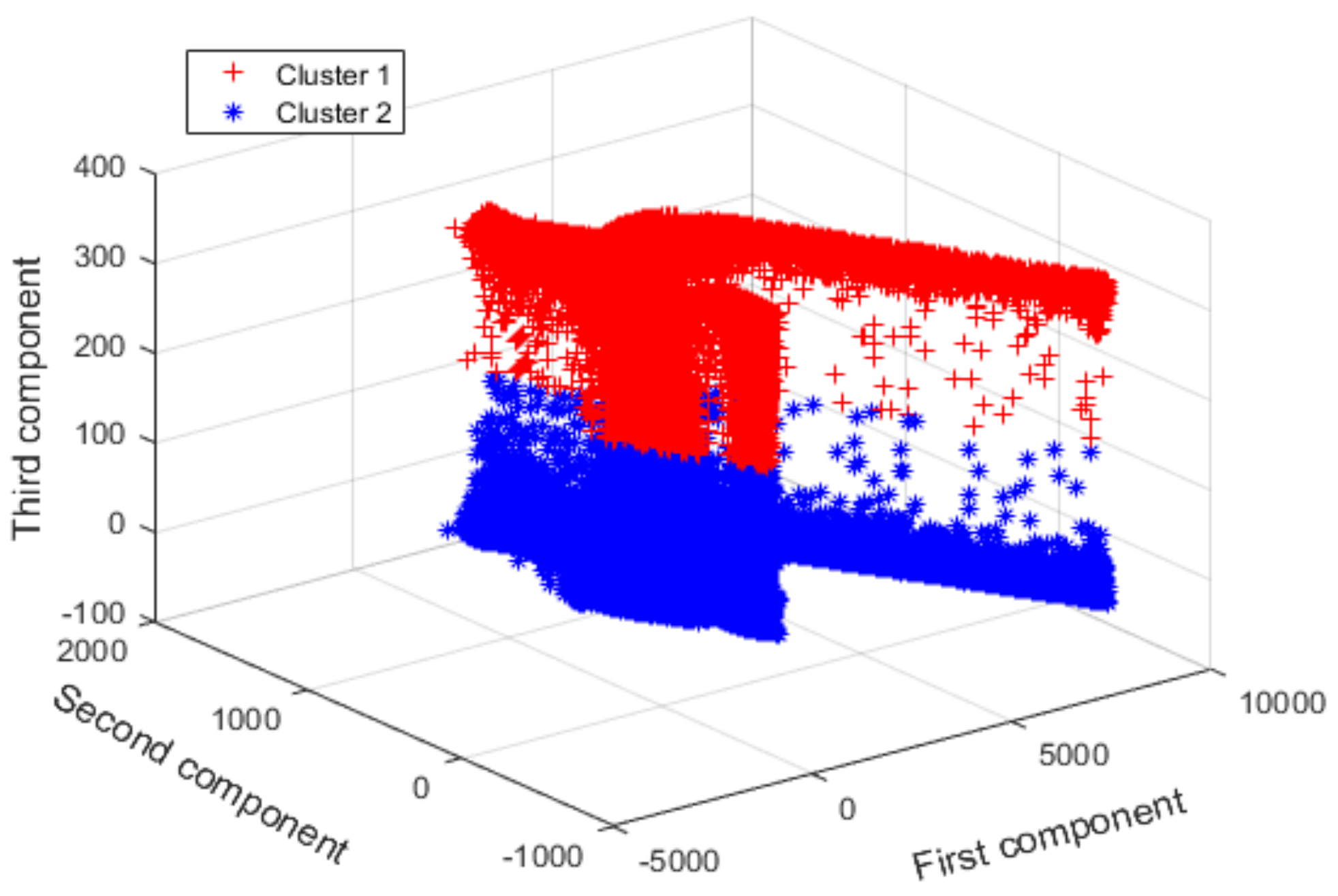
To explicitly show the optimal clustering results obtained, principal component analysis is used to reduce high-dimensional operation data to a low-dimensional space for data visualization. Figure 7 shows the three-dimensional visualization of the operation parameters based on the first three principal components. It can be clearly observed that two separate operation condition spaces are presented, which proves the multiple condition characteristics of wind turbines.

Table 3. Summary of clustering distribution.

Distribution	C1	C2
Wind speed (m/s)	0.3–29.28	0.3–25.33
Wind direction ($°$)	186.73–359	0.38–186.73
Ambient temperature ($°\mathrm{C}$)	4.97–37.33	4.96–37.58
Generator speed (rpm)	0.17–1852.8	0.17–1859.2
Generator torque ($\mathrm{N}\cdot \mathrm{m}$)	−970–8600	−970–8600

summarizes the clustering distribution of operation parameters to further quantitatively understand the clustering results.

As can be seen in Table 3, as far as the wind direction is concerned, the ranges under the two conditions are obviously different. In the case of C₁, the range is 186.73 to 359, whereas in C₂, the range is 0.38 to 186.73. In terms of wind speed, ambient temperature, generator speed, and generator torque, there is little difference in the ranges under the two conditions. One can see from the comparison results that the wind turbine operating conditions are clearly partitioned according to this operation parameter, i.e., wind direction, and thus this parameter can be used for subsequent real-time condition recognition purposes. However, it is well known that wind direction ranges from 0° to 360°, so here, if the wind direction is between 359°–360° and 0°–0.38°, they will be automatically categorized as C₁ and C₂ separately. It should be noted that there is no theoretical (i.e., no mechanical or electrical basis) reasoning for the choice of wind direction as the partitioning parameter here and that this based purely on the analysis of the clustering data.

In the following study, the original normal SCADA data from nine turbines are divided into two portions based on the above condition partition results, and the sample numbers under C₁ and C₂ are 154,089 and 199,042, respectively.

4.2.2. Parameter Selection for Each Condition Cluster

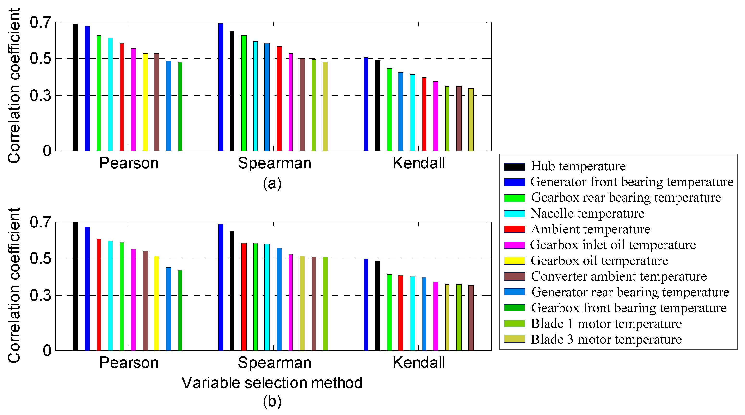
Before dealing with forecasting problems, the integration of Pearson, Spearman, and Kendall is used for variable selection. In this study, the main bearing temperature, closely related to the health of the main bearing, is taken as the target modeling variable for the output of each model. Meanwhile, state variables that are highly correlated with the main bearing temperature should be carefully considered. The correlation coefficients between the main bearing temperature listed in Table 1 and 48 other variables are calculated. There is no doubt that data preprocessing is required before calculating the correlation coefficients, including smoothing and normalization. Figure 8 shows the 10 most relevant variables for each method under the two conditions. For these three methods, it is essential to set a threshold according to the computation results, as shown in Figure 8, and in this paper, variables whose absolute value of the correlation coefficient is greater than 0.5 are selected as the final modeling input.

As shown in Figure 8a, in C₁, nine state variables are regarded as V₁ to construct the prediction model: hub temperature, generator front bearing temperature, gearbox rear bearing temperature, nacelle temperature, ambient temperature, gearbox inlet oil temperature, gearbox oil temperature, converter ambient temperature, and generator rear bearing temperature. As can be seen in Figure 8b, in addition to the nine input variables under C₁, blade 1 and 3 motor temperatures also meet the set threshold requirements, so 11 variables are considered to be V₂ to develop the regression model under C₂. Moreover, it is not difficult to see in Figure 8 that although the Kendall technique produces relatively small values under these two conditions, a similar ordering is generated compared to the first two approaches.

4.2.3. Performance Evaluation and Comparison

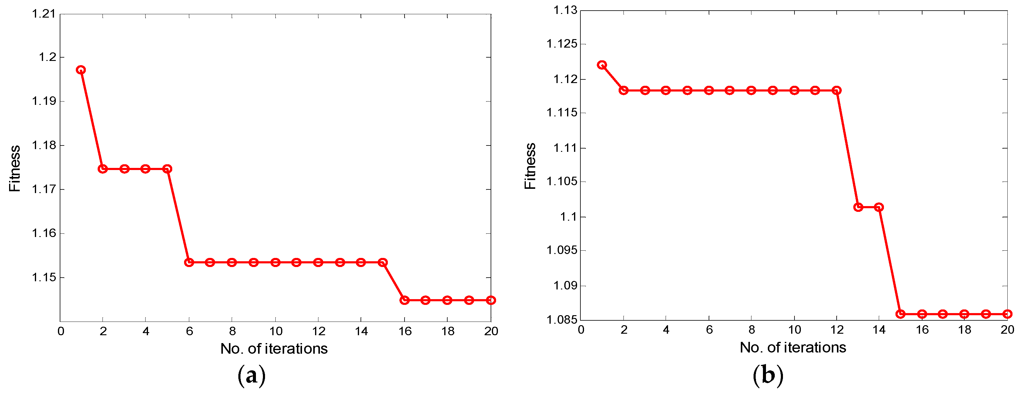
In this subsection, ODBNs are employed to develop a normal behavior model of each operating condition. In this study, four-layer DBNs are used for model development. To obtain higher prediction accuracy, the CSO algorithm is used to optimize the number of neurons in two hidden layers adaptively. Practically, a series of training parameters needs to be designed before establishing each normal behavior model. The detailed parameter settings are listed in

Table 4. Description of parameter settings for modeling.

Description	Parameter Setting
DBN pretraining phase	size of batch training 100, training iterations 10, learning rate 1, momentum 0
DBN fine-tuning phase	size of batch training 10, training iterations 20
CSO for optimization	max iterations 20, dimension 2, population size 20, range of each dimension [1, 100], updated frequency of chicken swarm 10, proportions of roosters, hens, and mother hens 0.15, 0.7, 0.5

. In each condition, the dataset is respectively divided into a training set, a validation set, and a testing set at a ratio of 80%, 10%, and 10%, respectively. The training set is utilized to train the DBN model, the validation set is applied to evaluate the performance of the model and optimize the fitness function, and the testing set is used for the final performance evaluation. Figure 9 shows the CSO optimization results under C₁ and C₂. The architecture of DBN₁ and DBN₂ is determined as 9-39-82-1 and 11-56-21-1, respectively.

In this study, to evaluate the prediction performance of the built model, four commonly used metrics, RMSE, mean absolute error (MAE), mean absolute percentage error (MAPE), and determination coefficient (R²), are adopted, which are defined as follows [43]:

$$\mathrm{RMSE}=\sqrt{\frac{1}{n}{\displaystyle \sum _{i=1}^n{(y_i-{\widehat{y}}_i)}^2}},$$

(19)

$$\mathrm{MAE}=\frac{1}{n}{\displaystyle \sum _{i=1}^n\left|y_i-{\widehat{y}}_i\right|},$$

(20)

$$\mathrm{MAPE}=\frac{1}{n}{\displaystyle \sum _{i=1}^n\left|\frac{y_i-{\widehat{y}}_i}{y_i}\right|}\times 100,$$

(21)

$${\mathrm{R}}^2=1-\frac{{\displaystyle \sum _{i=1}^n{(y_i-{\widehat{y}}_i)}^2}}{{\displaystyle \sum _{i=1}^n{(y_i-\overline{y})}^2}},$$

(22)

where $y_i$ represents the $i\mathrm{th}$ measured value, ${\widehat{y}}_i$ refers to the $i\mathrm{th}$ predicted value, and $\overline{y}$ is the mean value of the measurements.

Moreover, a back-propagation network with a single hidden layer (SHL-BP), a back-propagation network with double hidden layers (DHL-BP), and a support vector machine (SVM) are used for comparison. For SHL-BP and DHL-BP networks, the number of neurons in hidden layers is also optimized with CSO. For SVM, the radial basis kernel function is used to train the SVM model, and the kernel parameters and penalty factors are obtained by the cross-validation method. The quantitative evaluation results of the four models with three datasets under C₁ and C₂ are displayed in

Table 5. Comparison of prediction results. SHL-BP, back-propagation network with single hidden layer; DHL-BP, back-propagation network with double hidden layers; SVM, support vector machine; RMSE, root mean square error; MAE, mean absolute error; MAPE, mean absolute percentage error.

Dataset	Criteria	C1				C2
		SHL-BP1	DHL-BP1	SVM1	DBN1	SHL-BP2	DHL-BP2	SVM2	DBN2
Training	RMSE	1.9274	1.8044	1.8846	1.1463	1.8365	1.8325	1.9066	1.0858
	MAE	1.5034	1.4665	1.5361	0.8815	1.4444	1.4880	1.5696	0.8392
	MAPE (%)	0.6370	1.4872	0.7092	0.4393	0.3451	0.3097	0.9101	1.0432
	R2	0.7095	0.7454	0.7223	0.8973	0.7345	0.7356	0.7138	0.9072
Validation	RMSE	1.8908	1.8014	1.8898	1.1448	1.8333	1.8191	1.9108	1.0859
	MAE	1.4865	1.4627	1.5467	0.8822	1.4428	1.4731	1.5731	0.8329
	MAPE (%)	0.6054	1.4638	0.7382	0.3806	0.2916	0.3384	0.9469	0.9889
	R2	0.7219	0.7476	0.7222	0.8980	0.7348	0.7388	0.7119	0.9069
Testing	RMSE	1.9255	1.7982	1.8869	1.1607	1.8188	1.8198	1.9095	1.0790
	MAE	1.4941	1.4625	1.5390	0.8836	1.4319	1.4787	1.5694	0.8335
	MAPE (%)	0.6141	1.5531	0.7079	0.4485	0.3051	0.3315	0.9274	0.9726
	R2	0.7118	0.7486	0.7232	0.8953	0.7394	0.7391	0.7127	0.9083

.

It can be found from Table 5 that in the forecasting performance of C₁ for the training set, validation set, and testing set, DBN₁ is better than the SHL-BP₁, DHL-BP₁, and SVM₁ models, as it offers the lowest RMSE, MAE, and MAPE and highest R² values. In terms of the prediction results in C₂, DBN₂ produces the lowest RMSE and MAE values and the highest R² values in the three datasets, whereas MAPE is slightly higher than the other three models. As indicated from quantitative evaluation results, the ODBNs generally get a higher modeling accuracy than the three traditional methods. The main reason is that the SHL-BP network is based on the principle of empirical minimization, which is prone to fall into local minima during the training process and thus produces poor results. At the same time, because it is difficult to train the depth structure effectively with the BP algorithm, the prediction accuracy of the DHL-BP model is not much different from that of SHL-BP model. The SVM algorithm also obtains poor prediction results because it is not suitable for large-scale training samples, whereas ODBNs can deeply learn and uncover the sophisticated nonlinear relationships among modeling variables by establishing a depth model, which results in better prediction accuracy. Hence, the proposed ODBN approach is used for real-time health monitoring of main bearings under varying operating conditions.

Additionally, to evaluate the monitoring performance of the proposed multioperation condition framework, the same 353,131 samples are analyzed without considering the wind turbine operating characteristics. Similarly, the three variable selection methods mentioned in Section 3.3 are employed to select the modeling input variables. A total of 10 variables (gearbox oil temperature, gearbox inlet oil temperature, generator front bearing temperature, generator rear bearing temperature, converter ambient temperature, gearbox rear bearing temperature, ambient temperature, nacelle temperature, blade 1 motor temperature, and hub temperature) are selected. After that, the samples are split into the training set, validation set, and testing set, and four models are deployed to capture the normal behavior of the main bearings. Note that the division of the dataset and the optimization of the model parameters adopt the same way of considering the multi-condition operating characteristics. The prediction performances of the four models are summarized in

Table 6. Comparison results of four models without clustering.

Dataset	Evaluation Criteria	Model
		SHL-BP	DHL-BP	SVM	DBNs
Training	RMSE	1.9784	1.8538	1.8929	0.9615
	MAE	1.5959	1.4438	1.5574	0.7310
	MAPE (%)	0.0717	0.3721	0.7373	0.2933
	R2	0.6930	0.7305	0.7190	0.9275
Validation	RMSE	1.9737	1.8477	1.8879	0.9509
	MAE	1.5910	1.4397	1.5518	0.7242
	MAPE (%)	0.0907	0.3959	0.7543	0.2984
	R2	0.6941	0.7319	0.7201	0.9290
Testing	RMSE	1.9680	1.8470	1.8857	0.9536
	MAE	1.5852	1.4366	1.5518	0.7251
	MAPE (%)	0.0917	0.4039	0.7468	0.3066
	R2	0.6955	0.7318	0.7205	0.9285

.

As shown in Table 6, in terms of the training set, validation set, and testing set, the MAPE generated by the DBNs is slightly higher than the SHL-BP but lower than the DHL-BP and SVM models. Furthermore, the DBNs perform better with the lowest RMSE and MAE and highest R² values. As the results indicate, the ODBNs achieve the best prediction performance compared to the other three conventional models, illustrating the predominance of DBN method in modeling. Thus, it is deemed to be the more appropriate model for monitoring the main bearing temperature.

4.3. Health Monitoring Results

The examples given in this section are real wind turbine events from a wind farm recorded by SCADA systems. The MD is constructed to monitor the operating states of each wind turbine. The best performance algorithm for each condition is chosen to demonstrate the advantages of the proposed framework, and the monitoring performances are also compared with the best model considering only the single operating condition.

4.3.1. Testing Normal Wind Turbine Behavior

In this subsection, the proposed approach is used to analyze the normal behavior of wind turbines. Turbines 20 and 46 were in normal operation during 30 July to 2 August 2014 and 14–17 August 2014, respectively. The available historical SCADA data were collected and preprocessed for testing. The ODBN model was conducted for comparison. The prediction results with the two models are presented in

Table 7. Comparison of prediction results between two models.

Turbine	Model	Evaluation Criteria				Time (s)
		RMSE	MAE	MAPE (%)	R2
20	K-means based ODBNs	0.8125	0.6621	0.3725	0.9067	126.541
	ODBNs	0.8566	0.7021	0.7172	0.8963	4.308
46	K-means based ODBNs	1.5225	1.3038	4.1577	0.6272	124.126
	ODBNs	1.8409	1.5830	5.3136	0.4550	4.622

. The computational cost is also recorded in Table 7, with the computation environment Intel Core i7 CPU @1.73 GHz, and 8.00 GB memory.

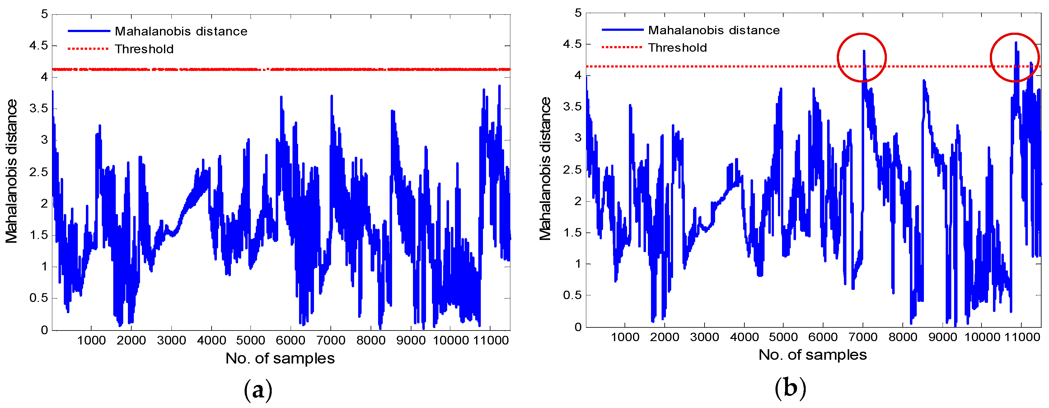
From Table 7, one can see that the models considering the operating condition characteristic produce lower RMSE, MAE, and MAPE and higher R² values for the two turbines than the model without this characteristic, which illustrates the superiority of the operating condition partition. In view of the better prediction performance of the proposed method, the loss of computational cost is acceptable. The condition monitoring results are displayed in Figure 10 and Figure 11.

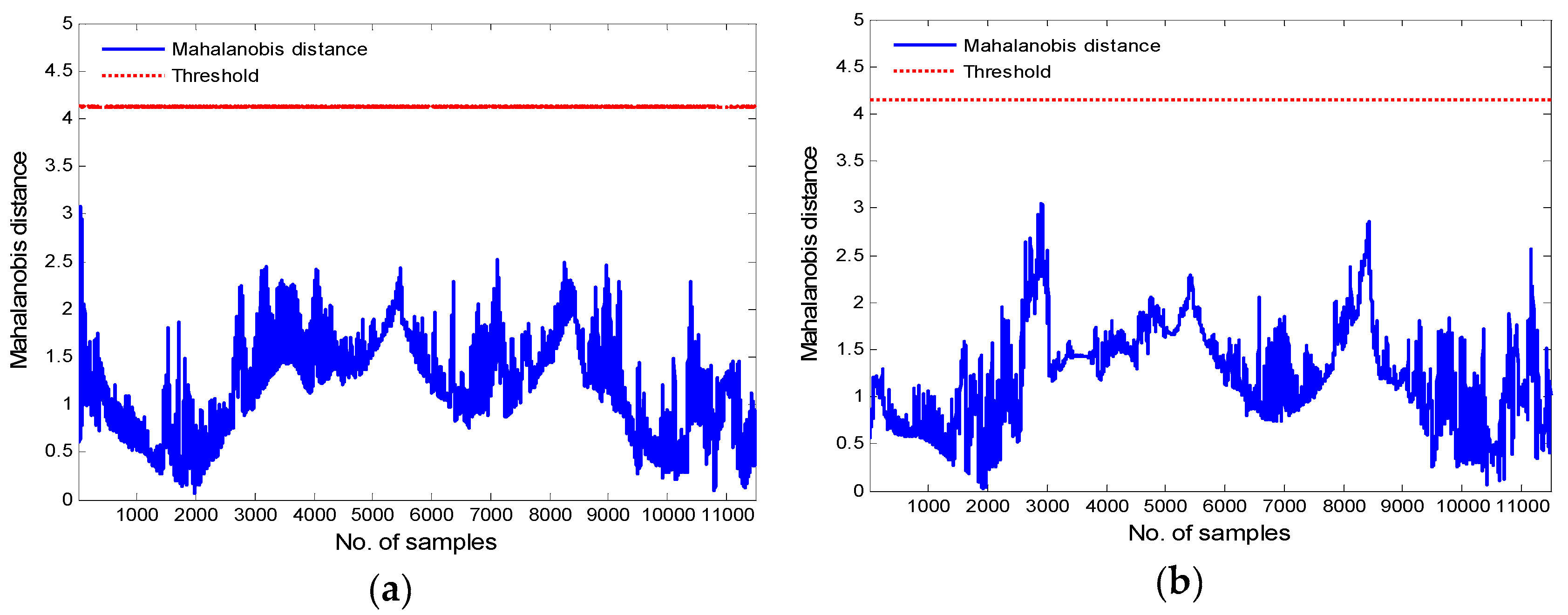
As can be seen from Figure 10a,b, all MD values of Turbine 20 fall within the detection thresholds, indicating that both methods can precisely capture normal wind turbine behavior. All MD values in Figure 11a are within the detection thresholds, whereas outliers are detected near points 7000 and 11,000 in Figure 11b. According to the monitoring results in Figure 11, the k-means based ODBN approach successfully monitors the operating state of Turbine 46 without false alarms, whereas the ODBN model produces false alarms. Hence, it can be concluded that the condition monitoring capability of the ODBN considering the operating condition feature is generally superior to that of the ODBN without that feature, and the fault thresholds under the two conditions, that is, MD₁ and MD₂ are 4.122 and 4.127, respectively. Since the two values in this study are not much different, they are approximated as straight in Figure 10a and Figure 11a.

4.3.2. Detecting Abnormal Main Bearing Behavior

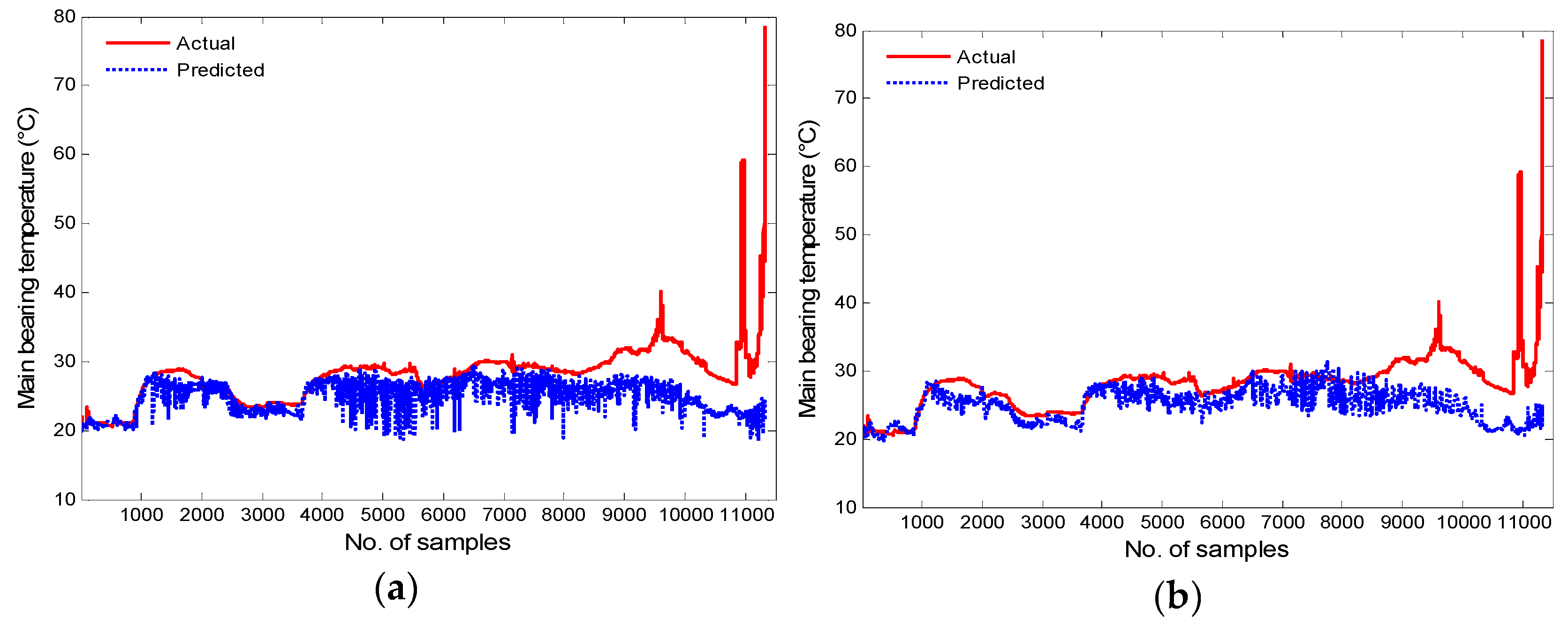
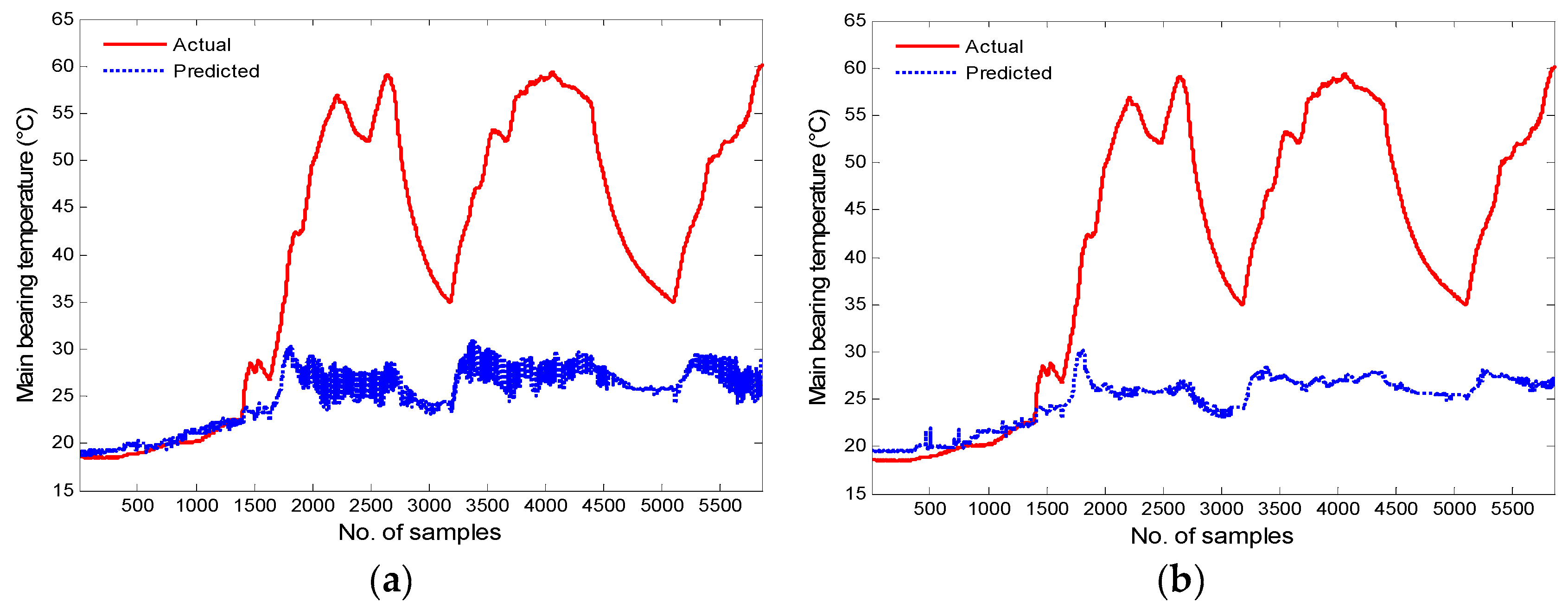
To further verify the effectiveness of the proposed approach in detecting the abnormal behavior of wind turbine main bearings, Turbines 42 and 13 are utilized for investigation. According to the SCADA records of Turbine 42, the main bearing over temperature fault occurred at 11:25 on 14 September 2014. The 11,324 SCADA samples from 12:50 on 10 September to 11:25 on 14 September before the event occurred are applied for anomaly detection. For Turbine 13, the 5855 SCADA samples from 00:00 on 2 July to 07:48 before the main bearing over temperature fault happened at 07:48 on 4 July are used for analysis. The ODBN model is used for comparison. The forecasting results with the two models are displayed in Figure 12 and Figure 13.

Figure 12 and Figure 13 demonstrate the trends of actual and predicted main bearing temperatures of Turbines 42 and 13 separately. It can be observed that the prediction errors between actual measured values and predicted values of the two models distinctly increased before the main bearing over temperature faults occurred, which indicates that the health conditions of the main bearings varied. The condition monitoring results are shown in Figure 14 and Figure 15.

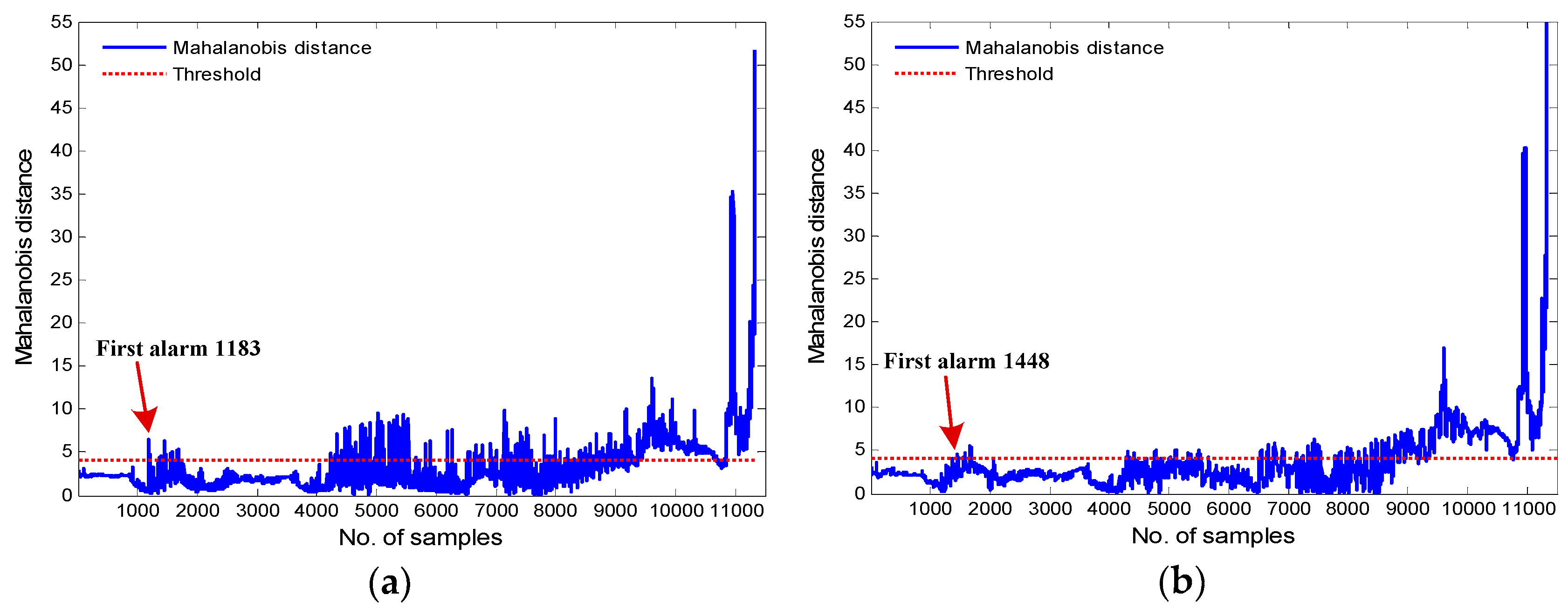
Figure 14a displays the monitoring results of the proposed framework for Turbine 42, while Figure 14b illustrates the monitoring results of the ODBN model in the same turbine. As shown in Figure 14a, the MD value first crosses the fault threshold at sample point 1183, and an incipient main bearing fault is detected. However, the actual fault occurred at 11:25 on 14 September 2014, which is the 11,325th sample point. Each sample point is separated by an interval of 30 s, so the k-means based ODBN approach can detect the main bearing fault approximately 84.5 h in advance. As can be seen from Figure 14b, the MD value first exceeds the threshold at sample point 1448, and an early alarm is signaled, thus predicting the over temperature event almost 82.3 h ahead of the actual fault. From the computation results in Figure 14, both models can identify the upcoming main bearing fault successfully. Nevertheless, the proposed k-means based ODBN model is able to detect the anomaly of the main bearing nearly 2.2 h earlier than the ODBN approach. At the same time, it also means that there is only a 2.2 h improvement in using the k-means based ODBN model over the ODBN model (82.3 vs. 84.5 h), which represents only a 2.6% improvement. Still, this can also provide more time for wind farm operators to take appropriate measures. If the abnormal main bearing can be repaired and replaced in time, possible major accidents and unnecessary maintenance costs and downtime can be avoided. The computational time of k-means based ODBN and ODBN methods during the condition monitoring is 129.596 s and 4.748 s, respectively.

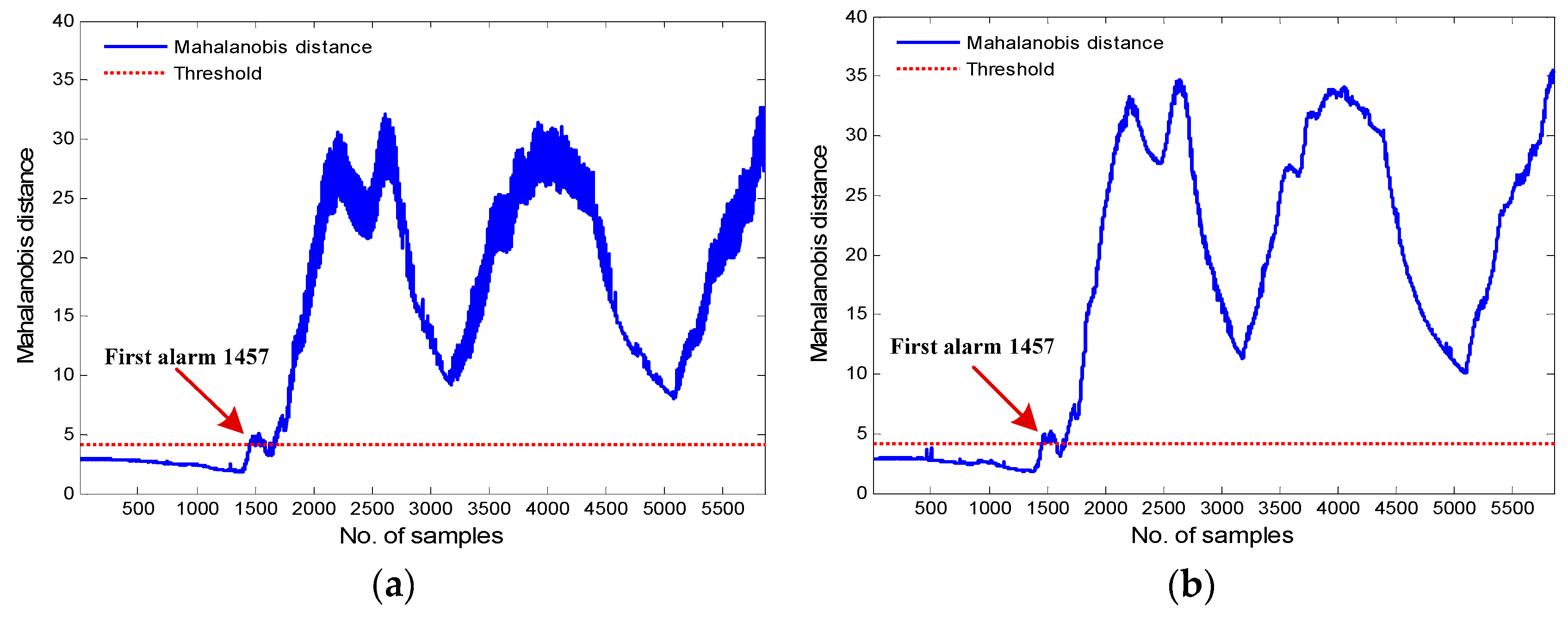
Figure 15a,b plot the monitoring results of the k-means–based ODBN and ODBN models, respectively, for Turbine 13. From Figure 15a, one can see that based on the fault thresholds, the alarm is first issued at sample point 1457, while the actual fault happened at 07:48 on 4 July 2014, which is the 5856th sample point. Therefore, the proposed approach can detect the fault almost 36.6 h in advance. As shown in Figure 15b, the MD value also first crosses the fault threshold at point 1457, and an early alarm is triggered. According to the computation results in Figure 15, one can conclude that the two models are able to simultaneously identify the anomaly of the main bearing nearly 36.6 h in advance, and the computational time of k-means-based ODBN and ODBN methods during the condition monitoring is 2.567 s and 68.046 s, respectively.

Based on the application analysis of the above real case, the proposed framework has certain advantages in the real-time health monitoring of wind turbines, which can mainly be attributed to the integration of multioperation condition monitoring and deep feature characterization. Meanwhile, the computational time is relatively high due to the complex procedures of the proposed divide-and-conquer strategy, but within acceptable limits. It is worth noting that the study is limited by the use of only three months of SCADA data and that the results are not valid for longer time periods.

5. Conclusions

A health monitoring method for wind turbine operational states has been proposed to consider the dynamic operating conditions of wind turbines and address the difficulty in accurately building normal behavior models. In the proposed approach, on the one hand, considering the multiple operating characteristics of wind turbines, a general multioperation condition partition scheme based on the k-means clustering method was utilized to segment the whole operation into multiple sub-operation conditions. One the other hand, ODBNs were applied to construct a healthy prediction model in each condition cluster where model parameters are optimally selected by the CSO algorithm. Compared with the conventional back-propagation and support vector machine models, the optimized modeling method can achieve higher prediction accuracy due to its deep feature representation capability.

A case for wind turbine main bearings was used to verify the effectiveness of the proposed health monitoring framework by real SCADA data. Compared with the ODBN model without considering the operating characteristics, the proposed framework does not generate false alarms under the normal conditions of wind turbines. In addition, both models are capable of detecting the anomalies of wind turbine main bearings in advance. Specifically, the proposed method could detect the faults either sooner, although only a 2.6% improvement, or at the same time. The results of normal and abnormal behavior testing demonstrate that the proposed approach generally achieves more effective and reliable detection accuracy.

This study also brings a loss of computational cost while having good detection performance. Also, due to data constraints, the study is limited by the use of only three months of SCADA data and the results are not valid for longer time periods. In future work, our developed framework will also be used for long-term monitoring of the main bearing operational states when more available SCADA data are collected. Other optimization methods will be used for the main bearing health monitoring. In addition, the approach will be extended to the application of other components in wind turbines.

References

- Global Wind Statistics 2017; Global Wind Energy Council (GWEC): Brussels, Belgium, 2018.
- Takoutsing, P.; Wamkeue, R.; Ouhrouche, M.; Slaoui-Hasnaoui, F.; Tameghe, T.A.; Ekemb, G. Wind turbine condition monitoring: State-of-the-art review, new trends, and future challenges. Energies 2014, 7, 2595–2630. [Google Scholar]
- Jiang, G.Q.; He, H.B.; Xie, P.; Tang, Y.F. Stacked multilevel-denoising autoencoders: A new representation learning approach for wind turbine gearbox fault diagnosis. IEEE. Trans. Instrum. Meas. 2017, 66, 2391–2402. [Google Scholar] [CrossRef]
- Antoniadou, I.; Manson, G.; Staszewski, W.J.; Barszcz, T.; Worden, K. A time–frequency analysis approach for condition monitoring of a wind turbine gearbox under varying load conditions. Mech. Syst. Signal Process. 2015, 64, 188–216. [Google Scholar] [CrossRef]
- Zhu, J.D.; Yoon, J.M.; He, D.; Bechhoefer, E. Online particle-contaminated lubrication oil condition monitoring and remaining useful life prediction for wind turbines. Wind Energy 2015, 18, 1131–1149. [Google Scholar] [CrossRef]
- Sanchez, P.; Mendizabal, D.; Gonzalez, K.; Zamarreno, C.R.; Hernaez, M.; Matias, I.R.; Arregui, F.J. Wind turbines lubricant gearbox degradation detection by means of a lossy mode resonance based optical fiber refractometer. Microsyst. Technol. 2016, 22, 1619–1625. [Google Scholar] [CrossRef]
- Yang, W.X.; Court, R.; Jiang, J.S. Wind turbine condition monitoring by the approach of SCADA data analysis. Renew. Energy 2013, 53, 365–376. [Google Scholar] [CrossRef]
- Kusiak, A. Break through with big data. Ind. Eng. 2015, 47, 38–42. [Google Scholar]
- Zaher, A.; McArthur, S.D.J.; Infield, D.J.; Patel, Y. Online wind turbine fault detection through automated SCADA data analysis. Wind Energy 2009, 12, 574–593. [Google Scholar] [CrossRef]
- Guo, P.; Infield, D.; Yang, X.Y. Wind turbine generator condition-monitoring using temperature trend analysis. IEEE Trans. Sustain. Energy 2012, 3, 124–133. [Google Scholar] [CrossRef]
- Kusiak, A.; Verma, A. Analyzing bearing faults in wind turbines: A data-mining approach. Renew. Energy 2012, 48, 110–116. [Google Scholar] [CrossRef]
- Schlechtingen, M.; Santos, I.F.; Achiche, S. Wind turbine condition monitoring based on SCADA data using normal behavior models. Part 1: System description. Appl. Soft Comput. 2013, 13, 259–270. [Google Scholar] [CrossRef]
- Schlechtingen, M.; Santos, I.F. Wind turbine condition monitoring based on SCADA data using normal behavior models. Part 2: Application examples. Appl. Soft Comput. 2014, 14, 447–460. [Google Scholar] [CrossRef]
- Bangalore, P.; Tjernberg, L.B. An artificial neural network approach for early fault detection of gearbox bearings. IEEE Trans. Smart Grid 2015, 6, 980–987. [Google Scholar] [CrossRef]
- Bangalore, P.; Letzgus, S.; Karlsson, D.; Patriksson, M. An artificial neural network-based condition monitoring method for wind turbines, with application to the monitoring of the gearbox. Wind Energy 2017, 20, 1421–1438. [Google Scholar] [CrossRef]
- Bi, R.; Zhou, C.K.; Hepburn, D.M. Detection and classification of faults in pitch-regulated wind turbine generators using normal behaviour models based on performance curves. Renew. Energy 2017, 105, 674–688. [Google Scholar] [CrossRef]
- Zhan, S.; Tao, Q.Q.; Li, X.H. Face detection using representation learning. Neurocomputing 2016, 187, 19–26. [Google Scholar] [CrossRef]
- Wang, Y.; Wang, X.G.; Liu, W.Y. Unsupervised local deep feature for image recognition. Inf. Sci. 2016, 351, 67–75. [Google Scholar] [CrossRef]
- Jiang, G.Q.; Xie, P.; He, H.B.; Yan, J. Wind turbine fault detection using a denoising autoencoder with temporal information. IEEE ASME Trans. Mechatron. 2018, 23, 89–100. [Google Scholar] [CrossRef]
- Yang, Z.X.; Wang, X.B.; Zhong, J.H. Representational learning for fault diagnosis of wind turbine equipment: A multi-layered extreme learning machines approach. Energies 2016, 9, 379. [Google Scholar] [CrossRef]
- Hinton, G.E.; Osindero, S.; Teh, Y.W. A fast learning algorithm for deep belief nets. Neural Comput. 2006, 18, 1527–1554. [Google Scholar] [CrossRef]
- Chen, H.Z.; Wang, J.X.; Tang, B.P.; Xiao, K.; Li, J.Y. An integrated approach to planetary gearbox fault diagnosis using deep belief networks. Meas. Sci. Technol. 2017, 28, 025010. [Google Scholar] [CrossRef]
- Wan, J.; Liu, J.F.; Ren, G.R.; Guo, Y.F.; Yu, D.R.; Hu, Q.H. Day-ahead prediction of wind speed with deep feature learning. Int. J. Pattern Recognit. Artif. Intell. 2016, 30, 1650011. [Google Scholar] [CrossRef]
- Chen, Z.Y.; Li, W.H. Multisensor feature fusion for bearing fault diagnosis using sparse autoencoder and deep belief network. IEEE Trans. Instrum. Meas. 2017, 66, 1693–1702. [Google Scholar] [CrossRef]
- Ren, H.; Chai, Y.; Qu, J.F.; Ye, X.; Tang, Q. A novel adaptive fault detection methodology for complex system using deep belief networks and multiple models: A case study on cryogenic propellant loading system. Neurocomputing 2018, 275, 2111–2125. [Google Scholar] [CrossRef]
- Shao, H.D.; Jiang, H.K.; Zhang, X.; Niu, M.G. Rolling bearing fault diagnosis using an optimization deep belief network. Meas. Sci. Technol. 2015, 26, 115002. [Google Scholar] [CrossRef]
- Unal, M.; Onat, M.; Demetgul, M.; Kucuk, H. Fault diagnosis of rolling bearings using a genetic algorithm optimized neural network. Measurement 2014, 58, 187–196. [Google Scholar] [CrossRef]
- Qiao, W.; Lu, D.G. A survey on wind turbine condition monitoring and fault diagnosis-Part I: Components and subsystems. IEEE Trans. Ind. Electron. 2015, 62, 6536–6545. [Google Scholar] [CrossRef]
- Kusiak, A.; Li, W.Y. The prediction and diagnosis of wind turbine faults. Renew. Energy 2011, 36, 16–23. [Google Scholar] [CrossRef]
- Lapira, E.; Brisset, D.; Davari Ardakani, H.; Siegel, D.; Lee, J. Wind turbine performance assessment using multi-regime modeling approach. Renew. Energy 2012, 45, 86–95. [Google Scholar] [CrossRef]
- Yang, H.H.; Huang, M.L.; Lai, C.M.; Jin, J.R. An approach combining data mining and control charts-based model for fault detection in wind turbines. Renew. Energy 2018, 115, 808–816. [Google Scholar] [CrossRef]
- Macqueen, J. Some methods for classification and analysis of multivariate observations. In Proceedings of the 5th Berkeley Symposium on Mathematical Statistics and Probability, Berkeley, CA, USA, 21 June–18 July 1965; pp. 281–297. [Google Scholar]
- Jain, A.K. Data clustering: 50 years beyond k-means. Pattern Recognit. Lett. 2010, 31, 651–666. [Google Scholar] [CrossRef]
- Rousseeuw, P. Silhouettes: A graphical aid to the interpretation and validation of cluster analysis. J. Comput. Appl. Math. 1986, 20, 53–65. [Google Scholar] [CrossRef]
- Mazidi, P.; Bertling Tjernberg, L.; Sanz Bobi, M.A. Wind turbine prognostics and maintenance management based on a hybrid approach of neural networks and a proportional hazards model. Proc. Inst. Mech. Eng. Part O J. Risk Reliab. 2017, 231, 121–129. [Google Scholar] [CrossRef]
- Fisher, R.A. Statistical methods for research workers. Int. J. Plant Sci. 1954, 21, 340–341. [Google Scholar]
- Best, D.J.; Roberts, D.E. Algorithm AS 89: The upper tail probabilities of Spearman’s rho. J. R. Stat. Soc. 1975, 24, 377–379. [Google Scholar] [CrossRef]
- Taylor, J.M.G. Kendall and Spearman correlation-coefficients in the presence of a blocking variable. Biometrics 1987, 43, 409–416. [Google Scholar] [CrossRef] [PubMed]
- Hinton, G.E. Training products of experts by minimizing contrastive divergence. Neural Comput. 2002, 14, 1771–1800. [Google Scholar] [CrossRef] [PubMed]
- Hinton, G.E. A practical guide to training restricted boltzmann machines. In Neural Networks: Tricks of the Trade; Springer: Berlin, Germany, 2012; Volume 7700, pp. 599–619. [Google Scholar]
- Meng, X.B.; Liu, Y.; Gao, X.Z.; Zhang, H.Z. A new bio-inspired algorithm: Chicken swarm optimization. In Swarm Intelligence; Springer International Publishing: Berlin, Germany, 2014; Volume 8794, pp. 86–94. [Google Scholar]
- Niu, G.; Singh, S.; Holland, S.W.; Pecht, M. Health monitoring of electronic products based on Mahalanobis distance and Weibull decision metrics. Microelectron. Reliab. 2011, 51, 279–284. [Google Scholar] [CrossRef]
- Bai, Y.; Sun, Z.Z.; Zeng, B.; Deng, J.; Li, C. A multi-pattern deep fusion model for short-term bus passenger flow forecasting. Appl. Soft Comput. 2017, 58, 669–680. [Google Scholar] [CrossRef]
Figure 1.
Operating characteristic curves of a wind turbine in normal conditions.
Figure 2.
Flowchart of the proposed health monitoring framework. SCADA, supervisory control and data acquisition; DBN, deep belief network; MD, Mahalanobis distance.
Figure 3.
Topological structure of a restricted Boltzmann machine (RBM).
Figure 4.
Structure of DBN with n hidden layers.
Figure 5.
Flowchart of optimized DBN with chicken swarm optimization (CSO).
Figure 6.
Calculation results of silhouette values.
Figure 7.
Optimal clustering results by k-means and silhouette index.
Figure 8.
Correlation coefficients with different variable selection methods for (a) C1 and (b) C2.
Figure 9.
CSO optimization results under C1 and C2: (a) CSO-DBN1 and (b) CSO-DBN2.
Figure 10.
Condition monitoring results for Turbine 20: (a) K-means–based ODBNs and (b) ODBNs.
Figure 11.
Condition monitoring results for Turbine 46: (a) K-means based ODBNs and (b) ODBNs.
Figure 12.
Forecasting results for Turbine 42: (a) K-means based ODBNs and (b) ODBNs.
Figure 13.
Forecasting results for Turbine 13: (a) K-means based ODBNs and (b) ODBNs.
Figure 14.
Condition monitoring results for Turbine 42: (a) K-means based ODBN and (b) ODBN.
Figure 15.
Condition monitoring results for Turbine 13: (a) K-means based ODBN and (b) ODBN.