Crack Patterns in Heterogenous Rocks Using a Combined Phase Field-Cohesive Interface Modeling Approach: A Numerical Study


1
Elasticity and Strength of Materials Group, School of Engineering, Universidad de Sevilla, 41092 Seville, Spain
2
Department of Building Structures and Geotechnical Engineering, Universidad de Sevilla, 41012 Seville, Spain
3
School of Mechanical Sciences, Indian Institute of Technology, Bhubaneswar 752050, India
4
IMT School for Advanced Studies Lucca, Piazza San Francesco 19, 55100 Lucca, Italy
*
Author to whom correspondence should be addressed.
Energies 2019, 12(6), 965; https://doi.org/10.3390/en12060965
Submission received: 26 November 2018
/
Revised: 27 February 2019
/
Accepted: 4 March 2019
/
Published: 13 March 2019
(This article belongs to the Special Issue Computational Methods of Multi-Physics Problems)
Abstract
:Rock fracture in geo-materials is a complex phenomenon due to its intrinsic characteristics and the potential external loading conditions. As a result, these materials can experience intricate fracture patterns endowing various cracking phenomena such as: branching, coalescence, shielding, and amplification, among many others. In this article, we present a numerical investigation concerning the applicability of an original bulk-interface fracture simulation technique to trigger such phenomena within the context of the phase field approach for fracture. In particular, the prediction of failure patterns in heterogenous rock masses with brittle response is accomplished through the current methodology by combining the phase field approach for intact rock failure and the cohesive interface-like modeling approach for its application in joint fracture. Predictions from the present technique are first validated against Brazilian test results, which were developed using alternative phase field methods, and with respect to specimens subjected to different loading case and whose corresponding definitions are characterized by the presence of single and multiple flaws. Subsequently, the numerical study is extended to the analysis of heterogeneous rock masses including joints that separate different potential lithologies, leading to tortuous crack paths, which are observed in many practical situations.
1. Introduction
Fracture events in geological materials are phenomena of notable importance for the safety and stability of geological masses. This is a relevant issue to engineering applications including tunneling procedures, hydraulic fracture for energy reservoirs, deep foundations, to name a few. Due to the advent of novel modeling techniques and the advances in the computational capabilities, the usage of numerical methods for reliable predictions of failure in rock masses has suffered a tremendous improvement in the last few years, becoming a plausible alternative for the analysis of geo-materials.
In this setting, the presence of flaws such as defects/discontinuities in rocks leads to a substantial reduction of the strength of rock mass, as compared to the intact rock. In line with linear elastic fracture mechanics (LEFM), the singular character of the stress field around flaws can induce the propagation of such defects when the stress state within the rock mass is altered, for instance due to a tunnel excavation. Therefore, the existence, initiation, and propagation of fracture not only affect the mechanical response of the rock mass, but also the construction of the engineering structures. This dependence of the strength and deformability of the rock mass upon the intact rock and the characteristic discontinuities (fracture and joints) make the deep understanding of such fracture processes a challenging task.
Stemming from the complex nature of the rock mass, according to [1,2], it is possible to distinguish between crack initiation and propagation phenomena. Crack initiation is defined as the process through which pre-existing flaws initiate in a confined region in the neighborhood of a crack tip. Crack propagation events are those processes by which the pre-existing cracks continue to grow after the initiation. Thus, propagation phases can lead to crack coalescence and/or crack branching or bifurcation, among different scenarios, depending on the characteristics of the rock mass and the external loading conditions. With the aim of achieving a deep understanding of these phenomena, a great deal of research has been conducted in literature to characterize the crack propagation in rocks, which are succinctly discussed from the experimental and numerical standpoints in Section 1.1 and Section 1.2, respectively.
1.1. Experimental Investigations
In a landmark investigation, Lajtai [3] performed numerous experimental tests on gypsum of Paris specimens, with single flaws at different inclinations with respect to the direction of the external load. These tests led to the identification of different fracture stages of the rock mass under uniaxial compression. Subsequently Ingraffea et al., [4] have extended the experiments on Limestone and Granodiorite specimens, by orienting the flaws at a particular angle. In [4], the authors reported that the completed crack growth sequence upon failure, which allowed the identification of a complete variety of failure modes. Some recent studies on rocks with several flaws, which were oriented following different inclinations, manifested the complex nature of fracture events in rocks with evident crack coalescence [5,6,7,8].
Recently, several researchers have studied the response of rock mass on crack arrest, considering: (i) the number of defects, () the relative inclination of the flaws and () the applied external loads. Mentionable studies on experimental methods have thoroughly investigated uniaxial and biaxial compression tests in rocks, through which it is possible to identify that these materials may experience a combination of flaw slippage onset and wing propagation, followed by secondary cracks (shear dominated) leading to subsequent potential coalescence [5,6,7,8,9,10]. In particular, Sagong and Bobet [11] distinguished 9 coalescence types of cracks in rock masses.
Nevertheless, it is worth mentioning that the experimental studies on this topic have been profusely exploited in recent decades. Standard methods are often limited due to notable difficulties in the simulation of general loading tests and the preparation of specimens for this purpose. Under these circumstances, traditional experimental procedures are also complemented with the use of digital image correlation (DIC) techniques and 3D printing methods [12], fostering a new perspective for the generation of specimens with desired attributes.
1.2. Numerical Investigations
As mentioned above, many of the previous experimental studies were focused on uniaxial or biaxial compressive loads, since the general loading conditions are difficult to reproduce in the laboratory. This fact motivated the development of computational methods which can potentially capture complex failure mechanisms in rocks. Moreover, numerical methods generally lead to notable cost savings, as compared to arduous experimental campaigns.
Modeling the physical behavior of fracture phenomena in geo-materials has been traditionally tackled using linear elastic fracture mechanics-based methodologies, due to their relative simplicity and representativeness, provided that the confining pressure and loading rate are sufficiently low. From the modeling point of view, previous experimental studies have been employed as reference investigations to calibrate the numerical methods and to provide a deeper insight into the physical processes associated with fracture events in rocks. However, several difficulties have been identified in order to capture the wide variety of failure modes of such materials under different loading cases such as bidirectional traction-compression, traction-shear loading among many others, which evolve from the complex crack path when it is unknown a priori. In addition, tracking such crack paths will be further complicated by the development of branching and coalescence evolutions, which are typical scenarios encountered in geo-materials.
For this purpose, numerous computational methods have been proposed in the last three decades, especially within the context of nonlinear finite element method (FEM) and boundary element method (BEM), to simulate the complex failure modes in rocks. Later on, advanced computational approaches such as: cracking particles method (CPM) [13,14,15], Peridynamics [16] and dual-horizon Peridynamics [17,18] are developed, which neither do not require an explicit representation of the discontinuities in the displacement field due to fracture nor crack tracking algorithms for the identification of the propagation path.
Exploiting the BEM-based techniques, Einstein and coauthors [19,20] have developed reliable modeling tools to predict crack growth under the loading conditions leading to fracture in Modes I and II, considering the specimens with one or more internal flaws. However, due to the inherent versatility of FEM-based techniques, they are often preferred for fracture applications over alternative methodologies. Within the current modeling techniques to simulate fracture events in solids using FEM, the following categories can be differentiated:
- Methods based on continuum damage mechanics (CDM) encompass the stiffness degradation, by defining a set of internal-damage variables [21]. In their local forms, CDM models suffer from well-known pathological sensitivity of the corresponding estimations on the spatial discretization (finite element mesh) due to the loss of ellipticity of the corresponding governing equations. To mitigate such deficiency, integral regularization schemes and gradient-enhanced formulations have been proposed [22,23,24,25,26], apart from the alternative procedures introduced by Areias and coauthors [27] by combining the local damage formulation with local re-meshing techniques.
- Explicit crack tools can be employed to envisage a strong discontinuity in the displacement field. They rely on either the enrichment of the nodal displacement field at the element level using the partition of unity methods (PUM) [28,29,30], or the enrichment of the strain field (enhanced FEM, E-FEM) [31,32,33,34].
Although the above-mentioned methods have been extensively employed to simulate fracture events in different engineering applications, they present several limitations, particularly to capture the onset of multiple cracks and their evolution, apart from tracking the intricate fracture scenarios including branching and coalescence. This latter aspect is of remarkable complexity in strong discontinuity techniques, which suffer from topological operative problems under such conditions.
Due to the advances in the computational capabilities in the last decade, a renovated interest on diffusive damage models complying with nonlocal representation has been witnessed, which endow a scalar-based evolution equation for the damage field. Especially suitable for brittle fracture events, the so-called phase field (PF) approach of fracture envisages a diffusive crack representation with a nonlocal character [42]. This new concept shares some common aspects with respect to CDM formulations via the definition of a scalar PF variable, which varies from 0 to 1, and triggers the stiffness degradation upon failure.
PF methods can be understood as a regularized version of the Griffith fracture approach [43], through the advocation of the -convergence [44,45,46], whereby a direct competition between the elastic and the fracture energies is constructed in an integrated global functional of the system. The corresponding minimization of such functional allows capturing the initiation, growth, and propagation of cracks in solids in a robust and reliable manner. Notable contributions in this direction are due to Francfort and Marigo and their coauthors from a fundamental standpoint, see [42,47] and the associated references. Additional formulations exploiting the PF approach for brittle fracture have been rigorously developed by Bourdin et al. [47,48]. Whereas, several modified models have been recently proposed complying with a thermodynamically consistent framework, e.g., see [49,50,51,52]. Exploiting this potential, posterior studies, the PF approach has been extended to fracture studies in thin-walled structures [53,54,55], ductile failure [56,57], cohesive fracture [58], dynamic applications [59,60], multi-physics environments [61,62,63]. Recently, this methodology has also been applied to study the initiation of fracture in rocks with multiple flaws [64,65,66].
1.3. Objectives and Organization
Due to the appealing features of the PF method for fracture, the main objective of this work is focused on the application of the PF method and its combination with the interface-like cohesive method to model fracture events in heterogeneous rocks [67]. The advocation of the methodology proposed in [68], which was originally developed by the authors, allows the possible interaction of rock masses with different lithologies, which are separated by a series of predefined discontinuities. The analysis and understanding of interfaces in rocks have always been the subject of a great impact in the research community due to their importance in practice. This stems from the fact that they possess a certain amount of cohesion due to interlocking and roughness, along with frictional responses in case of large sliding modifying the response of the rock mass [69]. Therefore, the aim of this research is to address the potential predictive capabilities of the combined PF-CZM for its application in rock fracture. Based on this interest, the proposed technique is first validated by reproducing experimental results concerning fracture of intact rock and subsequently extended to the analysis of heterogeneous media.
The manuscript is organized as follows: Section 2 summarizes the basic concepts of the PF method for bulk fracture, whereas, the corresponding simulations are presented in Section 3. Posteriorly, general details concerning the combined PF-CZM for triggering fracture events in heterogenous rock mass is outlined in Section 4. Some representative applications to illustrate the applicability of the proposed method are presented in Section 5. Finally, the main conclusions of the present study are given in Section 6.
2. Fundamentals of the Phase Field Approach for Brittle Fracture
The basic concepts of the PF approach for fracture in rocks are briefly introduced in this section. The current formulation advocates the methodology proposed in [47,49], therefore, detailed derivations are herewith omitted for brevity.
2.1. Basic Concepts
Within the context of multi-dimensional analysis, see Figure 1, we consider an arbitrary body in the Euclidean space of dimension , whose material points are denoted by the position vectors in the Cartesian setting. Body actions are identified by the vector . The delimiting boundary is defined such that , where and denote the boundary portions in which kinematic and static surface actions are prescribed, respectively, complying to: and . The kinematic field is denoted by , whereas the second-order Cauchy stress tensor is identified by . Boundary conditions in this arbitrary body render:
where is the outward normal to the body.
The PF approach for fracture envisages the definition of a scalar-based phase field variable , where × [48], which quantifies the stiffness degradation at the material point level, in order to smear out the sharp crack topology. The intact and fully deteriorated states are identified based on the value of the PF parameter, i.e., and , respectively. Therefore, adopts continuous values between 0 and 1. The one-dimensional PF approximation is given by the expression: , where l indicates the characteristic material length related to the material strength and governs the regularization width. According to [49], the PF problem is governed by:
where is the Laplacian of , and stands for the spatial gradient. At this point, relevant contributions on this matter are due to the contributions by Wu and coauthors [70,71,72], who extended the applicability the PF method for cohesive and length-scale insensitive fracture.
To account for the regularization, a crack density functional is defined, which can be estimated using the relation:
As discussed in [42,45,73], Equation (3) represents the crack surface , in the limit . Furthermore, to prevent crack healing upon unloading, the thermodynamic consistency condition given by , is required. The crack density functional can be then expressed as [49]:
The above definition of allows the approximation of the crack surface integral in the original Griffith formulation by a volume integral as follows:
Therefore, the total potential of the body can be split into the internal and external counterparts represented, and , respectively:
where the first term in the integral represents the elastic energy of the body and the second term accounts for the energy dissipation.
To simulate the crack growth under tensile load, we adopt the spectral decomposition of the infinitesimal strain tensor between its corresponding positive and negative counterparts [49]:
where and are the Lamé’s constants, and and respectively identify the tensile and compressive counterparts of the strain tensor. In Equation (7), the symbol represents the trace operator, while stands for the so-called Macaulay bracket: .
Finally, the degradation function , which introduces a stiffness deterioration with the growth of the defect (crack), can be defined as:
where is a residual stiffness parameter to prevent numerical instability issues for fully degraded states, i.e., when . Also, note that according to Equation (7a), the degradation function (Equation (8)) exclusively affects the positive part of the elastic energy of the body. Thus, the corresponding Cauchy stress tensor in a decomposed fashion for the PF formulation renders:
In the Equation (9), represents the second-order identity matrix and identify the positive and negative parts of the stress tensor.
2.2. Numerical Implementation
In this Section, the numerical implementation of the PF approach for the fracture of intact rock, within the context of nonlinear FEM are briefly addressed. In the sequel, the corresponding to bulk operators will be denoted by the label b in the superscript.
Based on the isoparametric interpolation, the LaGrangian shape functions at the element level , defined in the natural space , are used for the interpolation of the geometry (). The displacement field (), as well as the variation () and the linearization () of are defined as:
where n indicates the number of nodes at the element level, and y denotes the nodal coordinates and displacements, respectively, which are collected into the operator y . Accordingly, the interpolation functions are arranged into the vector form .
In the similar lines, the strain field (), its variation () and its linearization () can be approximated using the compatibility operator associated with the kinematic field:
Similarly, the interpolation of the PF variable (damage-like variable), its variation and linearization render:
where are the nodal values of the PF variable, which are arranged into the vector . The spatial gradient of the PF (), its variation () and its linearization () can be interpolated through the operator :
Therefore, the discrete version of Equation (6) at the element level, identified by the super-index , can be expressed as:
where the residual vector , in which, and represent the internal and external forces, respectively, given by:
Correspondingly, is the residual vector associated with the PF variable, which can be estimated as:
In this study, a staggered solution scheme in the form of Jacobi-type iterative procedure is adopted for the numerical treatment of the governing equations. Thus, the consistent linearization of Equation (14) yields the following coupled system [57]:
The particular forms of the matrices , , and are omitted here for brevity [74]. The numerical implementation of the PF approach is carried out within the framework of the FE codes FEAP and ABAQUS, by generating the user-defined element routines.
3. Bulk Failure Predictions
3.1. Validation of the Developed PF Approach for Fracture Using the Brazilian Splitting Test
The developed PF methodology for fracture of intact rocks is validated by comparing the results with the standard Brazilian splitting test reported in [64]. The Brazilian test is extensively employed to characterize the tensile strength of rocks. The geometric definition of the benchmark problem involves a specimen of diameter equal to 52 mm, see Figure 2a. Furthermore, the following material parameters are considered: Young’s modulus E = 31.5 GPa, Poisson’s ratio = 0.25 and = 100 J/m. Furthermore, the length scale in the PF approach can be related to the material strength of one-dimensional bar:
Therefore, in the current application, we set l = 1 mm. Half of the specimen is discretized using 55,452 elements, the simulations are performed by controlling the displacement. Figure 2b depicts the crack path estimated by implementing the present PF method in the ABAQUS platform, in line with [64]. During the simulations, it is observed that the crack initiated at the center of the disc, which agrees with the experimental evidence. Upon further loading, the initiated crack starts to grow towards the upper end of the Brazilian disc. From the qualitative standpoint, Figure 3 shows the experimental-numerical correlation, whereby a very satisfactory agreement can be observed along the loading path, as compared to the PF methods in [64]. In particular, the simulation response is characterized by a linear evolution until the abrupt failure and hence the fracture. Deviation of the simulated results from the experimental data is attributed to the absence of contact modeling features in the simulations.
3.2. Numerical Predictions of Rock Fracture: Estimation of Damage Patterns Various Load Cases for Specimens with Multiple Flaws
In this section, several examples are presented to illustrate the potential of the developed PF approach to simulate fracture phenomena in rock specimens, with an inclined echelon flaws (with respect to the horizontal direction), subjected to different load cases.
The basic geometry under consideration is a rock specimen with dimensions 200 mm × 200 mm, consisting of four inclined echelon flaws which can be simplified due to symmetry, to a quarter specimen of size 50 mm × 50 mm with a single inclined flaw, as shown in Figure 4. The adopted mechanical properties in the simulation are: , , and 0.1 mm [64]. The domain is discretized using first-order iso-parametric elements equipped with PF attributes, and a uniform mesh of size h = 0.2 mm. The specimen is subjected to displacements imposed along the vertical and horizontal directions, see Figure 4. In particular, the maximum vertical displacement is prescribed as 3 mm (tensile/compression), whereas can have different ratios with respect to depending on the specific case. Simulations are performed under controlled displacement, with a maximum displacement increment equal to mm using a monolithic PF formulation.
3.2.1. Uniaxial Compression Test
We first analyze the deformation patterns in a uniaxial compression test, which is achieved by specifying 3 mm, in several steps and 0, see Figure 4. Figure 5 shows the failure maps, highlighting the fracture patterns, when the specified displacement reaches 2.4 mm (left) and 2.78 mm (right), respectively. Moreover, according to Figure 5, two cracks are observed to first initiate around the tips of the flaw, which are subsequently propagated parallel to the loading direction. These predictions are in good agreement with experimental observations, see [64].
3.2.2. Uniaxial Tensile Test
In the next step, the fracture patterns in a uniaxial tensile test are captured using the developed PF approach. Therefore, a tensile load along the y direction equal to 3 mm, is specified on to the system shown in Figure 4. The simulation is carried out by specifying the displacement load in several steps. Figure 6a. shows the failure maps highlighting the fracture patterns, when the specified displacement reaches 2.4 mm (left) and 2.78 mm (right), respectively. As compared to Figure 5, the predicted crack pattern is perpendicular to the loading direction, which agrees with the results reported in [64].
To summarize, the estimated results from compression and tension tests, using the present PF method are in close agreement with the reported experimental results [64], illustrating the robustness of the proposed methodology.
3.2.3. Compressive-Traction and Traction-Traction Tests
To complement the previous results, the developed methodology is extended to predict the fracture patterns under compression-traction and traction-traction load cases. The particular load cases are achieved by suitably combining the imposed vertical and horizontal displacements.
Figure 6b,c depict the failure maps under uniaxial tensile load, vertical compression and horizontal traction with = −1 and vertical compression and horizontal traction cases, respectively, setting = −2.5 mm. Notable incidence of the external loadings with respect to the estimated crack patterns can be observed. Figure 6b,c correspond to the failure maps of the samples subjected to compression-traction loads with = −1 and = −2, respectively. Comparing Figure 6b,c, the applied horizontal displacement is observed to have a moderate influence on the final damage pattern, which is principally aligned with the vertical imposed displacement.
The analysis is also applied to samples subjected to tensile-tensile loads. Figure 7a–c correspond to the failure maps estimated by specifying the displacement ratios = 1, 2, and 10, respectively. We note that the predicted crack patterns evolve from a perfectly aligned path with the flaw orientation for = 1, to almost horizontal path for = 10. In line with previous cases, the estimated results agree with the reported results in [64].
4. Coupling the PF Approach for Rock Fracture and the Interface Cohesive Zone Model: Application to Heterogeneous Media
4.1. General Aspects
In many engineering applications, rock mechanics in particular, heterogenous media separated by existing interfaces are often observed. The simulation of fracture events in such media is a challenging task. In this context, a plausible alternative is the combined phase field-cohesive zone model (PF-CZM) numerical approach [68], where a consistent coupling between the PF approach for brittle fracture in the matrix and the interface crack model are proposed. This technique can be conceived as a new paradigm for the consistent coupling of damage events of different signature, allowing complex crack evolution with multiple branches.
The point of departure of the PF-CZM consists of the consideration of a system with a predefined crack and a prescribed interface , see Figure 8. A generic point of the interface is denoted by the vector . Considering the internal potential of the body (omitting the subscript to alleviate the notation), the governing functional of the system (Equation (6)) can be written as:
The main attribute of the current method renders the additive decomposition of the dissipative part of the functional into two components related to: (i) the fracture energy dissipated in the matrix rock, which is characterized by and is modeled using the PF method, and () the interface energy that identifies the crack propagation along the existing interfaces and is modeled using a cohesive zone representation. Correspondingly, the governing functional in Equation (21), can be rewritten as:
where is used to identify the displacement gaps between the two flanks of the interface, is a history parameter [58], and is the PF variable in the matrix.
In this work, we account for the tension cut-off interface behavior given in [68], whose apparent stiffness is modified by taking into consideration the matrix damage state in the surrounding region via . Moreover, it is worth mentioning that the interface fracture energy, Equation (22), can be decomposed into the corresponding contributions to the fracture Modes I and II in a 2D setting of analysis, which are represented by and , respectively.
According to [68], it is assumed that the critical interface opening () obeys a linear law with respect to the damage state in the matrix. Therefore, the following relation can be postulated: , where and . Then the traction-separation law at the interface (Figure 9 for mode I), are given by:
where and are the critical traction values associated with the fracture Modes I and II, respectively, g are the displacements whose sub-indices n and t refer to fracture Modes I and II, respectively.
Consequently, the apparent interface stiffnesses for both fracture modes as a function of the bulk damage render
where and represent for the interface stiffness corresponding to intact matrix rock, i.e., .
We adopt a quadratic-based fracture criterion for triggering propagation events, given by:
where and are the individual energy release rates (ERRs) for fracture Modes I and II, respectively, which take the form:
Critical values of the ERRs defined above are compared to their critical values via Equation (26), whereby and are the critical values, given by:
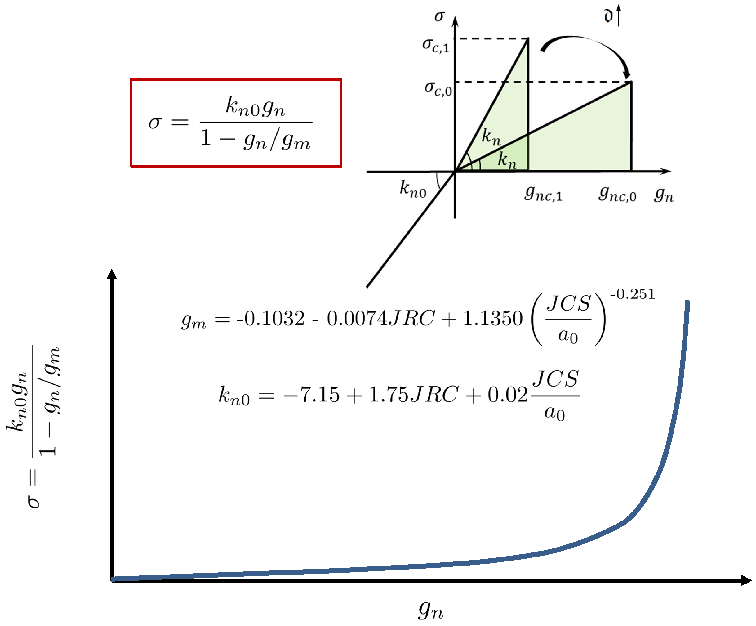
Finally, the interface formulation to encompass geo-mechanical aspects can be arrived in the similar lines of [75], where we incorporate a modified version of the normal penalty stiffness (to prevent inter-penetration between the interface flanks), which obeys the following hyperbolic expression:
where is the interface closure, is the initial stiffness, is the maximum interface closure. The values and , can be related in rock mechanics to the joint compressive strength (JCS), which is provided in the literature for many different geological masses, using the following correlations (Figure 9):
where JCS is the joint wall compression strength, which is the joint roughness coefficient introduced by Barton and Choubey [76], see also a recent overview on the use of this index in [77] and . These coefficients can be characterized by means of experimental campaigns on specific rock masses.
In line with the description of the current model, it is important to note that the independent parameters that characterize the interface response are: (i) the critical normal and tangential displacements corresponding to Mode I and II of fracture and , () the associated interface fracture energies and the fracture criterion, and () the corresponding geo-mechanical parameters. Additionally, the present model includes an additional capability that couples the apparent interface stiffness with respect to the PF (bulk) damage variable, and therefore two extra parameters are required corresponding to the pairs: , and , .
4.2. Variational Form and Finite Element Formulation
In this section, we present the particular aspects concerning the interface contribution to the total potential of the system, Equation (22). Following a standard Galerkin procedure, the weak form of the interface contribution can be expressed as:
where are the test functions of the displacement field , and stands for the test functions of the PF variable d.
The discretization of the present interface formulation is performed using first-order elements with linear interpolation functions. Thus, analogous to the PF approach for bulk fracture presented in Section 2.2, denotes the nodal displacement vector and is the phase field nodal vector, both at the element level. Accordingly, the discrete form of Equation (32) at the element level () renders:
The vector of displacement gaps () for any arbitrary point on the surface is the result of the difference in displacement vector between opposite flanks, which can be obtained from the displacement field by performing a pre-multiplication by the operator :
where is a matrix including the element shape functions of the displacement field and stands for the compatibility operator of the displacement field associated with the interface.
The transformation of the global gap vector into the local setting referred to the interface [38,41] is conducted via the rotation matrix from Equation (35) leading to the local gap vector , given by:
In a similar manner, the following discretization forms can be deduced for the average PF variable at the interface, at the element level as:
where is an operator computing the average value of the PF variable between the two interface flanks and identifies the corresponding compatibility operator. The specific forms of these matrices are given in [39,41].
Therefore, the discrete weak form renders
leading to the residual vectors:
Finally, through the directional derivative, the linearization of the residual vectors yields the following tangent matrices:
where:
and and are given by:
Please note that in line with Equation (19), the resulting coupled equations are solved using the monolithic Newton-Raphson scheme, obeying the form:
5. Fracture Analysis in Heterogeneous Rock Masses Using the PF-CZM Approach
5.1. General Considerations
The presence of interfaces in joint propagation is especially relevant in sedimentary rocks composed of siltstone and shale layers. The analysis of cracking events in multilayered materials has been a recurrent research in the last few years, as described in [68]. Similar to composite materials, there are three fundamental aspects of crucial importance in fracturing across interfaces, called joints in the rock mechanics literature: (i) the strength of the joint, () the material properties of the layers and () the loading conditions.
As discussed in [78], when an approaching crack impinges on a tough interface this crack generally tends to propagate into the adjacent bulk without experience significant deviations from its initial path. Conversely, weak joints are much more prone to fail, leading to noticeable delamination events. This basic scenario can be reproduced in a straightforward manner by the PF-CZM approach outlined in the previous section. Thus, Figure 10 qualitatively depicts the simulation of a homogeneous system of span L = 50 mm with the mechanical properties given above with a prescribed horizontal interface, which is then subjected to a uniform displacement at the lateral edges . We set the ratio between the fracture toughness of the bulk and the interface as = 50 for weak joint scenario, whereas, = 0.05 for tough joints. In this graph, it can be observed that the proposed PF-CZM faithfully reproduces the basic behavior discussed in [78]. Specifically, a discontinuous displacement map is shown for the weak joint case illustrating delamination events, whereas a well-defined crack front perpendicular to the loading direction is reproduced for the strong joint response.
However, for bi-material systems with weak joints, more complex situations can be encountered according to LEFM studies [68]. Particularly, three different propagation scenarios can be found based on the specific Dundurs’s parameters of the system when a crack impinges on an interface: (1) single deflection along the interface, (2) double deflection along the interface and (3) penetration. Figure 11 succinctly reproduces the results discussed in [68] using the current PF-CZ approach for a bi-material system subjected to uniform tensile load with a prescribed vertical joint between both media. Observing Figure 11, the numerical predictions led to very satisfactory qualitative agreement with respect to theoretical LEFM results in terms of fracture patterns for different values of the Dundurs’s parameter with respect to .
Relying on the illustrated potential capabilities, the next Sections addresses the applicability of the PF-CZ method to simulate fracture events in multilayered rock masses.
5.2. Application to Rock Salt Fracture with Inclined Interfaces
One of the potential applications of the developed numerical framework is the investigation of the response of bedded rocks salt. Particularly, these rocks perform in a different manner depending upon the corresponding lithology, which can obey either single or multi-layer arrangements. Following [79], mixed lithotypes present horizontal or inclined beds of anhydrite mudstone alternating with halite, leading to anhydrite-halite composite rocks.
From the experimental evidence in [79], it was observed that in such configurations, the presence of interlayers tends to promote crack initiation at this location, this fact being also promoted due to the inclined interface definition. Thus, these authors reported that typical failure sequence can be described by three different phases: (i) near/along the region of the interface, initial micro-defects stemming from the differences between sedimentation and consolidation evolve; () increasing the applied loading, such micro-cracks propagate along the interface and within the rock salt region; () finally, the coalescence of different crack occur, breaking the specimen.
The current numerical method is applied to study the deformation behavior and the fracture characteristics (initiation and coalescence) in bedded rocks salt with inclined interfaces under uniaxial compression in line with [79]. For this purpose, uniaxial compression simulations of composite rocks salt with interlayers of 20 mm in thickness are numerically analyzed, which showed a mechanical behavior close to brittle character. Due to the lack of reliable data regarding the geometry of the specimens analyzed in [79], the study is restricted to a qualitative investigation following a central interlayer disposal, see Figure 12. A domain of dimensions 100 × 200 mm is defined with a central interlayer of 20 mm in thickness following a macroscopic representation with two small flaws close to the interface. This domain is dsicretized using 84388 elements combining bulk and interface elements. The mechanical and fracture properties of both materials are listed in Table 1. Please note that for the interface between the rock salt and the anhydrite we choose an intermediate value between the transgranular boundary crack properties reported in [80], so that we set 1.2715 J/m.
Figure 12 depicts the qualitative numerical-experimental correlation of the predicted crack path of the current method and that observed in the experiments, showing a good qualitative agreement. In particular, during the simulations, it is observed that the main vertical cracks initiate at the flaws near the interface and propagate through the interlayer and subsequently both cracks propagate along the interface coalescing. The final failure pattern at this location agrees from a qualitative point of view with that reported in [79]. However note that the development of wing and shear crack paths are slightly deviated from the experimental evidence, so that alternative PF methods for bulk fracture as proposed in [65,66] can be employed in forthcoming studies. Nevertheless, a more comprehensive investigation falls beyond the scope of the current paper due to the lack of the required material data.
5.3. Numerical Investigation: Specimen with Multiple Flaws and Presence of Interfaces
Continuing with the assessment of the predictive capabilities of the current PF-CZM approach for heterogenous rock masses, we adopt the specimen definition described in Section 3, including the prescribed weak joints and multiple flaws with different lengths and orientations forming 45 with respect to the horizontal direction. Material properties of the specimens also replicate those given in Section 3. For the sake of conciseness in the results, we assume that the different lithologies are from the same material. Also note that bi- and tri-material systems can be directly analyzed using the current numerical methodology in a straightforward manner.
Additionally, with respect to the joint definitions that separate different bulk domains, we consider two cases: (i) a single horizontal joint, () a single vertical joint. Joint mechanical properties are given in Table 2, whereas, contact stiffness properties relying on geo-mechanical parameters are listed in Table 3.
It is worth mentioning that due to the lack of reliable experimental data, after validating the proposed method in the previous Sections, the present results are conducted to analyze the potential fracture patterns for different geometric characteristics and loading conditions.
5.3.1. Specimen with Two Inclined Flaws and a Horizontal Joint
The specific description of the flaw definitions within the domain, the joint positions and the loading conditions are shown in Figure 13a. The position of the joint coincides with the medial horizontal edge of the specimen. A compression-tension load case, where , with compression along the vertical direction is considered (we set 5 mm in the following analysis here presented) Figure 13b,c depict the predicted contour plots of the vertical displacement and the damage pattern at the end of the simulation. Analyzing the displacement field, Figure 13b, a clear discontinuity at the position of the joint can be appreciated. This fact indicates the occurrence of joint failure and therefore delamination. However, almost no increase in the value of PF variable within the specimen is predicted, see Figure 13c. These results clearly indicate that delamination along the existing joint can be identified as the predominant failure phenomenon for the given loading conditions.
To examine the clear influence of the applied loading on the failure characteristics, we analyze the specimen by prescribing the traction-traction loading conditions, i.e., through the definition of (both positive values along the corresponding edges based on the Cartesian setting given in the graph). The computed results clearly pinpoint a substantial change in the fracture conditions within the specimen, see Figure 14. In this case, the development of nucleation and propagation phases around the flaw tips are noticed. Upon load increasing, both crack events emanating from the flaws coalesce and subsequently reach the joint. A third phase in the failure path evolution is manifested by the crack propagations along the existing joint and subsequently progressing into the bottommost substrate, which concomitantly occurs with the crack propagation in the topmost substrate. These phenomena can be identified by analyzing the discontinuities in the contour map associated with the vertical displacement field and the PF evolution. This concomitant simulation of joint and bulk damage can be identified as one of the most appealing attributes of the present numerical methodology, since this allows interaction without user intervention throughout the computations. The simultaneous evolution of failure events from different signature during the analysis can be identified in Figure 14 regarding the load-displacement curve, whereby a first linear elastic evolution is followed by crack growth from the two flaws with incipient delamination along the interface in a later stage. Failure initiation is around 0.53.
Finally, for a most severe traction-traction case we define . Analyzing the contour map corresponding to the vertical displacement, Figure 15a, it is observed that for this loading configuration the crack pattern tends to progress with gradual change in its path. In particular, bulk fracture is reoriented along the direction of the flaws, and then reduce the extent of the delamination front, as seen in Figure 15b. This effect is also noticed above for the homogeneous crack example with a single inclined flaw, in Section 5.3. This behavior can be also noticed in the load-displacement evolution curve, Figure 15c, which in comparison with the previous case, the failure initiation is predicted to occur at around 0.5.
5.3.2. Specimen with Three Inclined Flaws
The previous analysis can be further extended to specimen definitions with 3 parallel flaws, 2 in the topmost substrate and 1 in the bottommost substrate. Moreover, regarding the joint position, we analyze the cases given by: (1) a single horizontal joint whose position is coincident with that described in the previous sections (Figure 16), and (2) a single vertical joint, placed at a distance of 20 mm with respect to the rightmost vertical edge, see Figure 18a.
With reference to the case with the horizontal interface under traction-traction loading conditions given by , it can be observed that the inclusion of the third flaw in the bottommost substrate of the model notably modifies the damage pattern. It is also noticed that the smallest flaw is not activated by the applied loading, and no damage events occur at the corresponding tips (Figure 16). Thus, crack phenomena are associated with the remaining larger flaws, featuring clear propagation paths which tend to coalesce. However, such two main cracks interact with the existing interface, and correspondingly the final damage pattern is a combination of bulk and interface failure. This sequence of damage can be identified analyzing the load-displacement curve (Figure 17) where different snapshots of the PF variable and the horizontal displacement are given. According to this graph, as usual, an initial linear evolution is depicted up to the fracture propagation of the main two flaws, which coincide with the first peak of the curve. Current results predict that these two main cracks initially propagate without involving any decohesion along the interface (note the continuity of the horizontal displacement field). However, when these two cracks are very close to the interface, they also induce the development of decohesion events, which are responsible for the final rupture of the specimen. This fact is characterized by the final abrupt failure in the load-displacement curve due to the tension cut-off interface model herein envisaged.
Regarding the vertical joint configuration, Figure 18b,c depict the final PF patterns for the cases and , respectively, showing completely different failure mechanisms in the predictions. Clear bulk failure emanating from the two larger flaws can be observed for the case , whereas the scenario setting shows that the main failure mechanism in this later specimen is due to joint decohesion. These two failure patterns can be confirmed by the analysis of the corresponding load-displacement curves, see Figure 19. Thus, the case features a standard evolution up to the first peak. At this point, the decohesion failure starts in unstable manner, followed by a second linear evolution up to the complete decohesion without any bulk failure, see the snapshot of the vertical displacements in Figure 19b. This response contrasts with that corresponding to the case , whereby the failure mechanism is due to the bulk failure without any interaction with the interface decohesion.
6. Conclusions
In this paper, the application of the combined PF-CZ approach for fracture heterogeneous in rock masses has been outlined with the incorporation of geo-mechanical parameters into the interface definition. The present methodology has been first validated for matrix rock damage, exhibiting an excellent accuracy with respect to experimental data. Subsequently, the developed method has been applied to the simulation of complex damage events in heterogeneous rock masses with weak joints and multiple flaws.
Results from the current model illustrate that the PF-CZ approach permits the prediction of crack initiation, propagation, coalescence, and branching in geo-materials in an autonomous manner without the necessity of user intervention. Moreover, differing from alternative PF formulations, its coupling with interface-like modeling techniques allows the characterization of tortuous crack patterns along predefined weak joints in such materials.
Future directions in this concern will regard the extension of the proposed method for anisotropic rocks, hydraulic fracture, porous media, and modified formulations for triggering shear failure.
Author Contributions
Conceptualization, J.R., P.D.; Methodology, J.R., M.P.; Investigation, P.R. Budarapu, J.R.; Resources, J.R.; Writing-Original Draft Preparation, J.R., P.R.B., M.P.; Writing-Review and Editing, J.R., P.R.B., M.P., P.D.; Funding Acquisition, J.R.
Funding
J. Reinoso is grateful to the support of the Spanish Ministry of Economy and Competitiveness/FEDER (Project MAT2015-71036-P).
Conflicts of Interest
The authors declare no conflict of interest.
References
- Hoek, E.; Bieniawski, Z.T. Brittle Fracture Propagation in Rock under Compression. Int. J. Fract. 1984, 26, 276–294. [Google Scholar] [CrossRef]
- Hoek, E. Brittle failure of rocks in rock mechanics in engineering practice. In Rock Mechanics in Engineering Practice; Stagg, K.G., Zienkiewicz, O.C., Eds.; Wiley: New York, NY, USA, 1968; pp. 99–124. [Google Scholar]
- Lajtai, E.Z. Brittle Fracture in Compression. Int. J. Fract. 1974, 10, 525–536. [Google Scholar] [CrossRef]
- Ingraffea, A.R.; Heuze, F.E. An Analysis of Discrete Fracture Propagation in Rock Loaded in Compression. In Proceedings of the 18th U.S. Symposium on Rock Mechanics, Keystone, Colorado, CO, USA, 22–24 June 1977. [Google Scholar]
- Suits, L.D.; Sheahan, T.C.; Wong, L.N.Y.; Einstein, H.H. Using high speed video imaging in the study of cracking processes in rock. Geotech. Test. J. 2009, 32, 164–180. [Google Scholar] [CrossRef]
- Bobet, A. Numerical simulation of initiation of tensile and shear cracks. In Proceedings of the DC Rocks (2001) the 38th US Symposium on Rock Mechanics (USRMS), Washington, DC, USA, 7–10 July 2011. [Google Scholar]
- Yang, S.Q.; Yang, D.S.; Jing, H.W.; Li, Y.H.; Wang, S.Y. An experimental study of the fracture coalescence behaviour of brittle sandstone specimens containing three fissures. Rock Mech. Rock Eng. 2012, 45, 563–582. [Google Scholar] [CrossRef]
- Reyes, O.; Einstein, H.H. Failure mechanisms of fractured rock—A fracture coalescence model. In Proceedings of the 7th International Conference on Rock Mechanics, International Society for Rock Mechanics, Aachen, Germany, 16–20 September 1991. [Google Scholar]
- Wong, L.; Einstein, H. Crack coalescence in molded gypsum and carrara marble: Part 1. Macroscopic observations and interpretation. Rock Mech. Rock Eng. 2009, 42, 475–511. [Google Scholar] [CrossRef]
- Wong, R.; Chau, K.; Tang, C.; Lin, P. Analysis of crack coalescence in rock-like materials containing three flaws—Part I: Experimental approach. Int. J. Rock Mech. 2001, 38, 909–924. [Google Scholar] [CrossRef]
- Sagong, M.; Bobet, A. Coalescence of multiple flaws in a rock-model material in uniaxial compression. Int. J. Rock Mech. Min. Sci. 2002, 39, 229–241. [Google Scholar] [CrossRef]
- Ma, G.W.; Dong, Q.Q.; Fan, L.F.; .Gao, J. An investigation of non-straight fissures cracking under uniaxial compression. Eng. Fracture Mechanics 2018, 15, 300–310. [Google Scholar] [CrossRef]
- Rabczuk, T.; Belytschko, T. Cracking particles: A simplified meshfree method for arbitrary evolving cracks. Int. J. Numer. Meth. Eng. 2004, 61, 2316–2343. [Google Scholar] [CrossRef]
- Rabczuk, T.; Belytschko, T. A three-dimensional large deformation meshfree method for arbitrary evolving cracks. Comput. Methods Appl. Mech. Eng. 2007, 196, 2777–2799. [Google Scholar] [CrossRef] [Green Version]
- Rabczuk, T.; Zi, G.; Bordas, S.; Nguyen-Xuan, H. A simple and robust three-dimensional cracking-particle method without enrichment. Comput. Methods Appl. Mech. 2010, 199, 2437–2455. [Google Scholar] [CrossRef]
- Rabczuk, T.; Ren, H. A peridynamics formulation for quasi-static fracture and contact in rock. Eng. Geol. 2017, 225, 42–48. [Google Scholar] [CrossRef]
- Ren, H.; Zhuang, X.; Cai, Y.; Rabczuk, T. Dual-horizon peridynamics. Int. J. Numer. Meth. Eng. 2016, 108, 1451–1476. [Google Scholar] [CrossRef] [Green Version]
- Ren, H.; Zhuang, X.; Rabczuk, T. Dual-horizon peridynamics: A stable solution to varying horizons. Comput. Methods Appl. Mech. Eng. 2017, 318, 762–782. [Google Scholar] [CrossRef] [Green Version]
- Bobet, A.; Einstein, H.H. Fracture coalescence in rock-type materials under uniaxial and biaxial compression. Int. J. Rock Mech. Min. Sci. 1998, 35, 863–888. [Google Scholar] [CrossRef]
- Gonçalves da Silva, B.; Einstein, H.H. Modeling of crack initiation, propagation and coalescence in rocks. Int. J. Fract. 2013, 182, 167–186. [Google Scholar] [CrossRef] [Green Version]
- Lemaitre, J.; Desmorat, R. Engineering Damage Mechanics: Ductile, Creep, Fatigue and Brittle Failures; Springer-Verlag: Berlin, Germany, 2005. [Google Scholar]
- Bažant, Z.P.; Pijaudier-Cabot, T.G.P. Nonlocal continuum damage, localization instability and convergence. J. Appl. Mech. 1988, 55, 287–293. [Google Scholar] [CrossRef]
- Jirásek, M. Nonlocal models for damage and fracture: Comparison of approaches. Int. J. Solids Struct. 1988, 35, 4133–4145. [Google Scholar] [CrossRef]
- Forest, S. Micromorphic approach for gradient elasticity, viscoplasticity, and damage. J. Engnr. Mech. 2009, 35, 117–131. [Google Scholar] [CrossRef]
- Dimitrijevic, B.J.; Hackl, K. A regularization framework for damage-plasticity models via gradient enhancement of the free energy. Int. J. Numer. Methods Biomed. Energy 2011, 27, 1199–1210. [Google Scholar] [CrossRef]
- Peerlings, R.; Geers, M.; de Borst, R.; Brekelmans, W. A critical comparison of non local and gradient-enhanced softening continua. Int. J. Solids Struct. 2001, 38, 7723–7746. [Google Scholar] [CrossRef]
- Areias, P.; Msekh, M.A.; Rabczuk, T. Damage and fracture algorithm using the screened Poisson equation and local remeshing. Eng. Fract. Mech. 2016, 158, 116–143. [Google Scholar] [CrossRef]
- Moës, N.; Dolbow, J.; Belytschko, T. A finite element method for crack growth without remeshing. Int. J. Numer. Methods Eng. 1999, 46, 131–150. [Google Scholar] [CrossRef]
- Dolbow, J.; Moeës, N.; Belytschko, T. An extended finite element method for modeling crack growth with contact. Comput. Meth. Appl. Mech. Eng. 2001, 190, 6825–6846. [Google Scholar] [CrossRef]
- Fries, T.P.; Belytschko, T. The extended/generalized finite element method: An overview of the method and its applications. Int. J. Numer. Methods Eng. 2010, 84, 253–304. [Google Scholar] [CrossRef]
- Simo, J.C.; Oliver, J.; Armero, F. An analysis of strong discontinuities induced by strainsoftening in rate-independent inelastic solids. Comput. Mech. 1993, 12, 277–296. [Google Scholar] [CrossRef]
- Linder, C.; Armero, F. Finite elements with embedded strong discontinuities for the modeling of failure in solids. Int. J. Numer. Methods Eng. 2007, 72, 1391–1433. [Google Scholar] [CrossRef]
- Oliver, J.; Huespe, A.; Blanco, S.; Linero, D. Stability and robustness issues in numerical modeling of material failure with the strong discontinuity approach. Comput. Methods Appl. Mech. Eng. 2006, 195, 7093–114. [Google Scholar] [CrossRef]
- Armero, F.; Linder, C. New finite elements with embedded strong discontinuities for finite deformations. Comput. Methods Appl. Mech. Eng. 2008, 197, 3138–3170. [Google Scholar] [CrossRef]
- Xu, X.P.; Needleman, A. Numerical simulation of fast crack growth in brittle solids. J. Mech. Phys. Solids 1994, 42, 1397–1434. [Google Scholar] [CrossRef]
- Ortiz, M.; Pandolfi, A. Finite deformation irreversible cohesive elements for three-dimensional crack-propagation analysis. Int. J. Num. Meth. Eng. 1999, 44, 1267–1282. [Google Scholar] [CrossRef]
- Park, K.; Paulino, G.H.; Roesler, J.R. A unified potential-based cohesive model of mixed-mode fracture. J. Mech. Phys. Solids 2009, 57, 891–908. [Google Scholar] [CrossRef]
- Paggi, M.; Wriggers, P. Stiffness and strength of hierarchical polycrystalline materials with imperfect interfaces. J. Mech. Phys. Solids 2012, 60, 557–572. [Google Scholar] [CrossRef]
- Reinoso, J.; Paggi, M. A consistent interface element formulation for geometrical and material nonlinearities. Comput. Mech. 2014, 54, 1569–1581. [Google Scholar] [CrossRef] [Green Version]
- Infuso, A.; Corrado, M.; Paggi, M. Image analysis of polycrystalline solar cells and modelling of intergranular and transgranular cracking. J. Eur. Ceram. Soc. 2015, 34, 2713–2722. [Google Scholar] [CrossRef]
- Paggi, M.; Reinoso, J. An anisotropic large displacement cohesive zone model for fibrillar and crazing of interfaces. Int. J. Solids Struct. 2015, 69, 106–120. [Google Scholar] [CrossRef]
- Francfort, G.A.; Marigo, J.J. Revisiting brittle fracture as an energy minimization problem. J. Mech. Phys. Solids 1998, 46, 1319–1342. [Google Scholar] [CrossRef]
- Griffith, A.A. The phenomena of rupture and flow in solids. Philos. Trans. Royal Soc. Lond. A 1921, 221, 163–198. [Google Scholar] [CrossRef]
- Ambrosio, L.; Tortorelli, V.M. Approximation of functional depending on jumps by elliptic functional via C-convergence. Commun. Pure Appl. Math. 1990, 43, 999–1036. [Google Scholar] [CrossRef]
- Ambrosio, L.; Tortorelli, V.M. On the approximation of free discontinuity problems. Boll. Union Mat. Ital. 1992, 6, 105–123. [Google Scholar]
- Dal Maso, G. Introduction to Γ-Convergence. Progress in Nonlinear Differential Equations and Their Applications, Birkhäuser. Progress in Nonlinear Differential Equations and Their Applications. Available online: https://link.springer.com/book/10.1007/978-1-4612-0327-8 (accessed on 13 March 2019).
- Bourdin, B.; Francfort, G.A.; Marigo, J.J. Numerical experiments in revisited brittle fracture. J. Mech. Phys. Solids 2000, 48, 797–826. [Google Scholar] [CrossRef]
- Bourdin, B.; Francfort, G.A.; Marigo, J.J. The variational approach to fracture. J. Elast. 2008, 91, 145–148. [Google Scholar] [CrossRef]
- Miehe, C.; Hofacker, M.; Welschinger, F. A phase field model for rateindependent crack propagation: Robust algorithmic implementation based on operator splits. Comput. Methods Appl. Mech. Eng. 2010, 199, 2765–2778. [Google Scholar] [CrossRef]
- Miehe, C.; Welschinger, F.; Hofacker, M. Thermodynamically consistent phasefield models of fracture: Variational principles and multi-field fe-implementations. Int. J. Numer. Methods Eng. 2010, 83, 1273–1311. [Google Scholar] [CrossRef]
- Kuhn, C.; Müller, R. A continuum phase field model for fracture. Eng. Fract. Mech. 2010, 77, 3625–3634. [Google Scholar] [CrossRef]
- Borden, M.J.; Hughes, T.J.R.; Landis, C.M.; Verhoosel, C.V. A higher-order phase-field model for brittle fracture: Formulation and analysis within the isogeometric analysis framework. Comput. Methods Appl. Mech. Eng. 2014, 273, 100–118. [Google Scholar] [CrossRef]
- Amiri, F.; Millán, D.; Shen, Y.; Rabczuk, T.; Arroyo, M. Phase-field modeling of fracture in linear thin shells. Theor. Appl. Fract. Mech. 2014, 69, 102–109. [Google Scholar] [CrossRef] [Green Version]
- Areias, P.; Rabczuk, T.; Msekh, M.A. Phase-field analysis of finite-strain plates and shells including element subdivision. Comput. Methods Appl. Mech. Eng. 2016, 312, 322–350. [Google Scholar] [CrossRef]
- Reinoso, J.; Paggi, M.; Linder, C. Phase field modeling of brittle fracture for enhanced assumed strain shells at large deformations: Formulation and finite element implementation. Comp. Mech. 2017. [Google Scholar] [CrossRef]
- Ulmer, H.; Hofacker, M.; Miehe, C. Phase field modeling of brittle and ductile fracture. Proc. Appl. Math. Mech. 2013, 13, 533–536. [Google Scholar] [CrossRef]
- Ambati, M.; Gerasimov, T.; de Lorenzis, L. Phase-field modeling of ductile fracture. Comp. Mech. 2015, 55, 1–24. [Google Scholar] [CrossRef]
- Verhoosel, C.; de Borst, R. A phase-field model for cohesive fracture. Int. J. Numer. Meth. Eng. 2013, 96, 43–62. [Google Scholar] [CrossRef]
- Borden, M.J.; Verhoosel, C.V.; Scott, M.A.; Hughes, T.J.R.; Landis, C.M. A phase-field description of dynamic brittle fracture. Comput. Methods Appl. Mech. Eng. 2012, 217–220, 77–95. [Google Scholar] [CrossRef]
- Hofacker, M.; Miehe, C. A phase field model of dynamic fracture: Robust field updates for the analysis of complex crack patterns. Int. J. Numer. Methods Eng. 2013, 93, 276–301. [Google Scholar] [CrossRef]
- Miehe, C.; Schanzel, L.; Ulmer, H. Phase field modeling of fracture in multi-physics problems. Part I. Balance of crack surface and failure criteria for brittle crack propagation in thermo-elastic solids. Comput. Methods Appl. Mech. Eng. 2015, 294, 449–485. [Google Scholar] [CrossRef]
- Miehe, C.; Schanzel, L.; Ulmer, H. Phase field modeling of fracture in multi-physics problems. Part II. Coupled brittle-to-ductile failure criteria and crack propagation in thermo-elastic solids. Comput. Methods Appl. Mech. Eng. 2015, 294, 486–522. [Google Scholar] [CrossRef]
- Martínez-Pañeda, E.; Golahmar, A.; Niordson, C.F. A phase field formulation for hydrogen assisted cracking. Comput. Methods Appl. Mech. Eng. 2018, 342, 742–761. [Google Scholar] [CrossRef]
- Zhou, S.; Zhuang, X.; Zhu, H.; Rabczuk, T. Phase field modelling of crack propagation, branching and coalescence in rocks. Theor. Appl. Fract. Mech. 2018, 96, 174–192. [Google Scholar] [CrossRef]
- Zhang, X.; Sloan, S.W.; Vignes, C.; Sheng, D. A modification of the phase-field model for mixed mode crack propagation in rock-like materials. Comput. Methods Appl. Mech. Eng. 2017, 322, 123–136. [Google Scholar] [CrossRef]
- Bryant, E.C.; Sun, W. A mixed-mode phase field fracture model in anisotropic rocks with consistent kinematics. Comput. Methods Appl. Mech. Eng. 2018, 342, 561–584. [Google Scholar] [CrossRef]
- Li, L.; Xia, Y.; Huang, B.; Zhang, L.; Li, M.; Li, A. The Behaviour of Fracture Growth in Sedimentary Rocks: A Numerical Study Based on Hydraulic Fracturing Processes. Energies 2016, 9, 169. [Google Scholar] [CrossRef]
- Paggi, M.; Reinoso, J. Revisiting the problem of a crack impinging on an interface: A modeling framework for the interaction between the phase field approach for brittle fracture and the interface cohesive zone model. Comput. Methods Appl. Mech. Eng. 2017, 321, 145–172. [Google Scholar] [CrossRef]
- Carpinteri, A.; Paggi, M. Size-scale effects on strength, friction and fracture energy of faults: A unified interpretation according to fractal geometry. Rock Mech. Rock Eng. 2008, 41, 735–746. [Google Scholar] [CrossRef]
- Wu, J.Y. A unified phase-field theory for the mechanics of damage and quasi-brittle failure in solids. J. Mech. Phys. Solids 2017, 103, 72–99. [Google Scholar] [CrossRef]
- Wu, J.Y.; Nguyen, V.P. A length scale insensitive phase-field damage model for brittle fracture. J. Mech. Phys. Solids 2018, 119, 20–42. [Google Scholar] [CrossRef]
- Nguyen, V.P.; Wu, J.Y. Modeling dynamic fracture of solids using a phase-field regularized cohesive zone model. Comput. Methods Appl. Mech. Eng. 2018, 340, 1000–1022. [Google Scholar] [CrossRef]
- Amor, H.; Marigo, J.J.; Maurini, C. Regularized formulation of the variational brittle fracture with unilateral contact: Numerical experiments. J. Mech. Phys. Solids 2009, 57, 1209–1229. [Google Scholar] [CrossRef]
- Msekh, M.A.; Sargado, M.; Jamshidian, M.; Areias, P.; Rabczuk, T. Abaqus implementation of phase-field model for brittle fracture. Comput. Mater. Sci. 2015, 96, 472–484. [Google Scholar] [CrossRef]
- Lei, Q.; Latham, J.P.; Xiang, J. Implementation of an emprirical joint constitutive model into finite-discrete element analysis of the geomechanical behavior of fractured rocks. Rock Mech. Rock Eng. 2016, 49, 4799–4816. [Google Scholar] [CrossRef]
- Barton, N.; Choubey, V. The shear strength of rock joints in theory and practice. Rock Mech. 1977, 10, 1–54. [Google Scholar] [CrossRef]
- Barton, N. Shear strength criteria for rock, rock joints and rock masses: Problems and some solutions. J. Rock Mech. Geotech. Eng. 2013, 5, 249–261. [Google Scholar] [CrossRef]
- Helgeson, D.E.; Aydin, A. Characteristics of joint propagation across layer interfaces in sedimentary rocks. J. Struct. Geol. 1991, 13, 897–911. [Google Scholar] [CrossRef]
- Li, Y.; Liu, W.; Yang, C.; Daemen, J.J.K. Experimental investigation of mechanical behavior of bedded rock salt containing inclined interlayer. Int. J. Rock Mech. Min. Sci. 2014, 69, 39–49. [Google Scholar] [CrossRef]
- Tromans, D.; Meech, J.A. Fracture toughness and surface energies of minerals: Theoretical estimates for oxides, sulphides, silicates and halides. Miner. Eng. 2002, 15, 1027–1041. [Google Scholar] [CrossRef]
Figure 1.
Regularization of the sharp crack topology within the spirit of the phase field approach for fracture.
Figure 1.
Regularization of the sharp crack topology within the spirit of the phase field approach for fracture.

Figure 2.
(a) Brazilian splitting test: loading condition. (b) Damage pattern of the specimen.

Figure 3.
Brazilian splitting test: Load-displacement evolution curve.

Figure 4.
Specimen with inclined flaws: geometry and loading conditions.

Figure 5.
Uniaxial compression case: Failure pattern at an initial stage (a) and at advanced stage (b).
Figure 5.
Uniaxial compression case: Failure pattern at an initial stage (a) and at advanced stage (b).

Figure 6.
Different loading scenarios for a specimen with a single flaw: predicted damage patterns. (a) Uniaxial tensile case. (b) Vertical compression and horizontal traction with = −1. (c) Vertical compression and horizontal traction with = −2.
Figure 6.
Different loading scenarios for a specimen with a single flaw: predicted damage patterns. (a) Uniaxial tensile case. (b) Vertical compression and horizontal traction with = −1. (c) Vertical compression and horizontal traction with = −2.

Figure 7.
Different tensile-tensile loading scenarios for a specimen with a single flaw: predicted damage patterns. (a) Vertical traction and horizontal traction with = 1. (b) Vertical traction and horizontal traction with = 2. (c) Vertical traction and horizontal traction with = 10.
Figure 7.
Different tensile-tensile loading scenarios for a specimen with a single flaw: predicted damage patterns. (a) Vertical traction and horizontal traction with = 1. (b) Vertical traction and horizontal traction with = 2. (c) Vertical traction and horizontal traction with = 10.
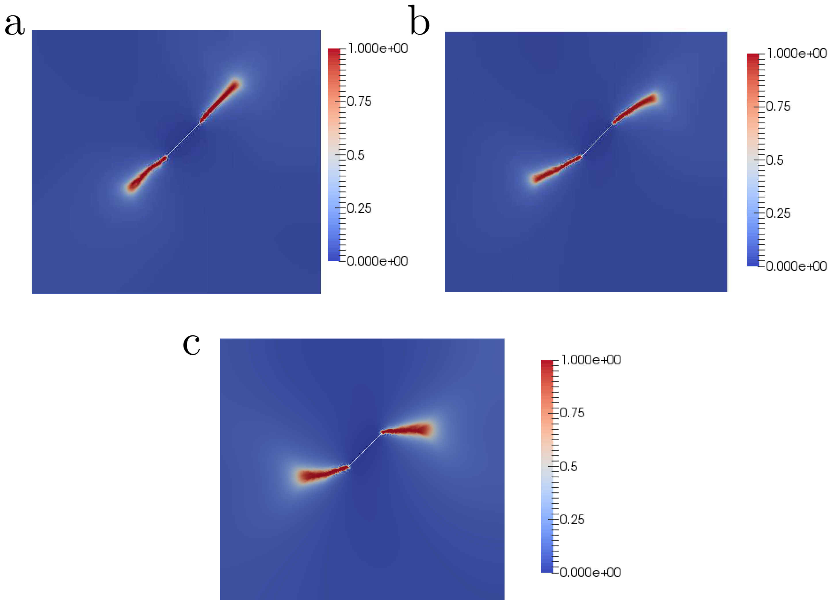
Figure 8.
Coexistence between brittle fracture in the bulk and cohesive debonding of an interface within the context of the phase field approach of fracture.
Figure 8.
Coexistence between brittle fracture in the bulk and cohesive debonding of an interface within the context of the phase field approach of fracture.

Figure 9.
Modification of interface penalty stiffness under normal compression due to geo-mechanical aspects: schematic representation under negative normal gap .
Figure 9.
Modification of interface penalty stiffness under normal compression due to geo-mechanical aspects: schematic representation under negative normal gap .

Figure 10.
String system subjected to uniaxial displacement. Predictions using PF-CZM for two types of interfaces between similar materials: weak joints with delamination events along the interface and strong joints with continuous crack path.
Figure 10.
String system subjected to uniaxial displacement. Predictions using PF-CZM for two types of interfaces between similar materials: weak joints with delamination events along the interface and strong joints with continuous crack path.

Figure 11.
Geometry and boundary conditions for the bi-material problem. Crack pattern scenarios for brittle interface. The contour plots of the dimensionless vertical displacement field correspond to three different cases labeled A (double deflection), B (single deflection), C (penetration).
Figure 11.
Geometry and boundary conditions for the bi-material problem. Crack pattern scenarios for brittle interface. The contour plots of the dimensionless vertical displacement field correspond to three different cases labeled A (double deflection), B (single deflection), C (penetration).

Figure 12.
Salt rock composite specimen under uniaxial compressive loading. Geometry and boundary conditions, experimental failure pattern and numerical predictions.
Figure 12.
Salt rock composite specimen under uniaxial compressive loading. Geometry and boundary conditions, experimental failure pattern and numerical predictions.

Figure 13.
(a) Specimen with 2 inclined flaws and a horizontal joint. Case : (b) horizontal displacement field; (c) damage pattern.
Figure 13.
(a) Specimen with 2 inclined flaws and a horizontal joint. Case : (b) horizontal displacement field; (c) damage pattern.

Figure 14.
Specimen with 2 inclined flaws and a horizontal joint. Case traction-traction: (a) vertical displacement; (b) damage pattern; (c) Load-displacement evolution curve including snapshots of the phase field variable.
Figure 14.
Specimen with 2 inclined flaws and a horizontal joint. Case traction-traction: (a) vertical displacement; (b) damage pattern; (c) Load-displacement evolution curve including snapshots of the phase field variable.

Figure 15.
Specimen with 2 inclined flaws and a horizontal joint. Case traction-traction: (a) vertical displacement; (b) damage pattern; (c) Load-displacement evolution curve including snapshots of the phase field variable.
Figure 15.
Specimen with 2 inclined flaws and a horizontal joint. Case traction-traction: (a) vertical displacement; (b) damage pattern; (c) Load-displacement evolution curve including snapshots of the phase field variable.

Figure 16.
(a) Specimen with 3 inclined flaws and a horizontal joint. (b) Phase field damage pattern at the end of the simulation.
Figure 16.
(a) Specimen with 3 inclined flaws and a horizontal joint. (b) Phase field damage pattern at the end of the simulation.
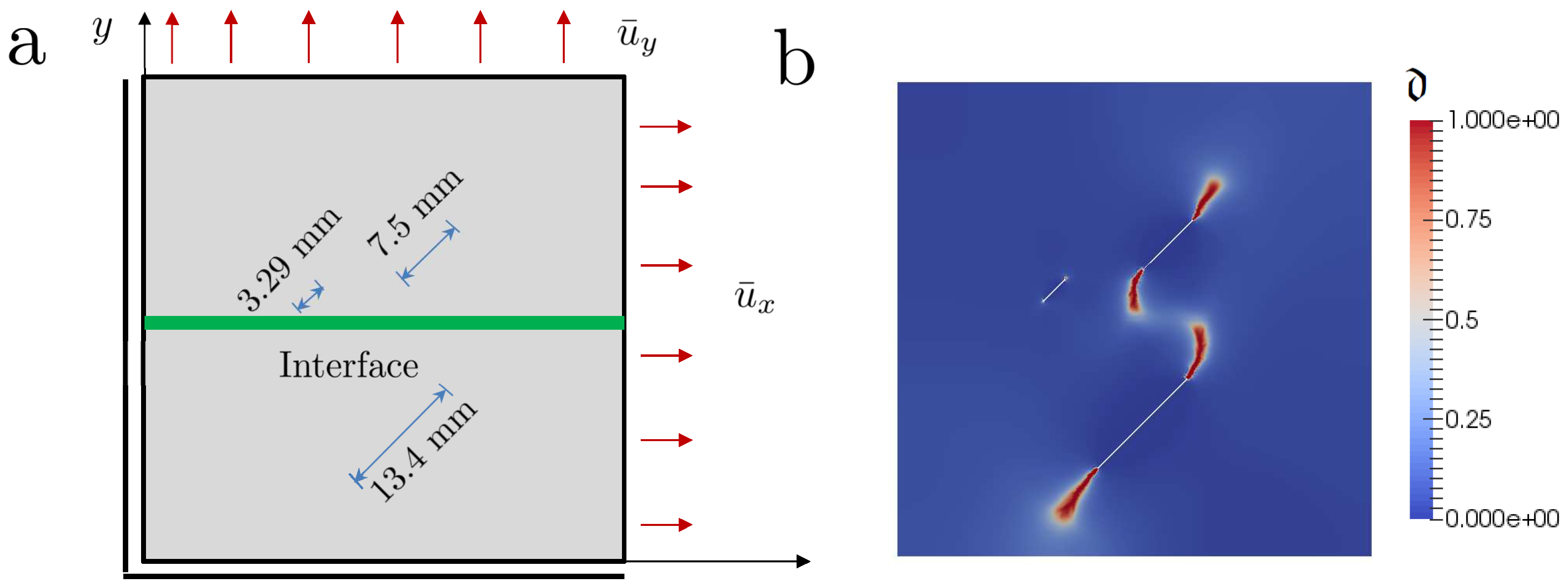
Figure 17.
Specimen with 3 inclined flaws and a horizontal joint. Load-displacement evolution curve including snapshots of the bulk (phase field) failure and the horizontal displacement fields.
Figure 17.
Specimen with 3 inclined flaws and a horizontal joint. Load-displacement evolution curve including snapshots of the bulk (phase field) failure and the horizontal displacement fields.

Figure 18.
Specimen with 3 inclined flaws and a vertical interface: (a) Loading and geometric description. (b) Phase field pattern for . (c) Phase field pattern for .
Figure 18.
Specimen with 3 inclined flaws and a vertical interface: (a) Loading and geometric description. (b) Phase field pattern for . (c) Phase field pattern for .

Figure 19.
Specimen with 3 inclined flaws and a vertical interface: (a) Load-displacement curve for . (b) Load-displacement curve for .
Figure 19.
Specimen with 3 inclined flaws and a vertical interface: (a) Load-displacement curve for . (b) Load-displacement curve for .


Table 1.
Mechanical and fracture properties: halite and anhydrite.
| Material | E (GPa) | (Jm) | |
|---|---|---|---|
| Halite | 36.87 | 0.254 | 1.155 |
| Anhydrite | 74.36 | 0.269 | 1.805 |
Table 2.
Interface fracture properties.
| Critical traction Mode I interface | 75 MPa |
| Critical traction Mode II interface | 90 MPa |
| Fracture toughness Mode I | 0.002 N/mm |
| Fracture toughness Mode II | 0.008 N/mm |
Table 3.
Penalty stiffness properties of the joint based on geo-mechanical aspects.
| 10 | |
| 0.194 mm | |
| JCS | 169 MPa |
| JRC | 9.7 |
| Friction angle | 32º |
| 0.2 m |
© 2019 by the authors. Licensee MDPI, Basel, Switzerland. This article is an open access article distributed under the terms and conditions of the Creative Commons Attribution (CC BY) license (http://creativecommons.org/licenses/by/4.0/).
Share and Cite
MDPI and ACS Style
Reinoso, J.; Durand, P.; Budarapu, P.R.; Paggi, M. Crack Patterns in Heterogenous Rocks Using a Combined Phase Field-Cohesive Interface Modeling Approach: A Numerical Study. Energies 2019, 12, 965. https://doi.org/10.3390/en12060965
AMA Style
Reinoso J, Durand P, Budarapu PR, Paggi M. Crack Patterns in Heterogenous Rocks Using a Combined Phase Field-Cohesive Interface Modeling Approach: A Numerical Study. Energies. 2019; 12(6):965. https://doi.org/10.3390/en12060965
Chicago/Turabian StyleReinoso, José, Percy Durand, Pattabhi Ramaiah Budarapu, and Marco Paggi. 2019. "Crack Patterns in Heterogenous Rocks Using a Combined Phase Field-Cohesive Interface Modeling Approach: A Numerical Study" Energies 12, no. 6: 965. https://doi.org/10.3390/en12060965
Note that from the first issue of 2016, this journal uses article numbers instead of page numbers. See further details here.