Characterizing Flexoelectricity in Composite Material Using the Element-Free Galerkin Method


1
Division of Computational Mechanics, Ton Duc Thang University, 700000 Ho Chi Minh City, Viet Nam
2
Faculty of Civil Engineering, Ton Duc Thang University, 700000 Ho Chi Minh City, Viet Nam
3
College of Civil Engineering, Tongji University, 1239 Siping Road, Shanghai 200092, China
4
Institute of Continuum Mechanics, Leibniz Universität Hannover, Appelstr. 11, 30167 Hannover, Germany
*
Author to whom correspondence should be addressed.
Energies 2019, 12(2), 271; https://doi.org/10.3390/en12020271
Submission received: 30 October 2018
/
Revised: 9 December 2018
/
Accepted: 11 December 2018
/
Published: 16 January 2019
(This article belongs to the Special Issue Computational Methods of Multi-Physics Problems)
Abstract
:This study employs the Element-Free Galerkin method (EFG) to characterize flexoelectricity in a composite material. The presence of the strain gradient term in the Partial Differential Equations (PDEs) requires continuity to describe the electromechanical coupling. The use of quartic weight functions in the developed model fulfills this prerequisite. We report the generation of electric polarization in a non-piezoelectric composite material through the inclusion-induced strain gradient field. The level set technique associated with the model supervises the weak discontinuity between the inclusion and matrix. The increased area ratio between the inclusion and matrix is found to improve the conversion of mechanical energy to electrical energy. The electromechanical coupling is enhanced when using softer materials for the embedding inclusions.
1. Introduction
An energy harvester utilizing the electromechanical coupling effect has been applied in various applications, ranging from sensors [1,2,3] to biomedical devices [4,5] at both micro- and nano-scales [6,7,8]. The well-known electromechanical coupling effect, piezoelectricity, generates the electrical polarization under mechanical deformation only in the non-centrosymmetric material. Flexoelectricity is another type of electromechanical coupling, which describes the coupling between the electrical potential and strain gradient. Unlike piezoelectricity, flexoelectricity can exist in any dielectric material regardless of the material’s inner structure. In the meantime, experimental studies [9,10] observed an unexpected giant flexoelectric effect in barium strontium titanate, which suggested that at the micro-/nano-scale, the flexoelectric effect outperforms the piezoelectric effect. These superior properties of flexoelectricity at a small scale have drawn extensive research attention towards the fundamental investigation of this electromechanical coupling from the molecular scale to the continuum scale. Atomic-level density functional theories [11,12,13] and molecular dynamics simulations [14,15] explored the mechanism of inducing flexoelectric polarization under deformation. However, continuum scale studies can lead to better understanding of the practical applicability of the flexoelectric property in designing sensors and actuators.
The characterization of flexoelectricity with existing numerical methods, like the Finite Element Method (FEM), requires remarkable modifications to handle the strain gradient term. Zhang et al. [16] used conventional FEM to evaluate the piezo- and flexo-electric effects by solving the partial differential equations for the displacement and electric potential in a decoupled manner. The conventional FEM works on the basis of continuity and is uncertain when higher order strain terms are present (challenging to hold continuity). Nanthakumar et al. [17,18] used the Mixed Finite Element Formulation (MFEF) to maximize the flexoelectric effect through topology optimization of barium titanate material. However, the MFEF method suffers from high computational cost [19,20]. Isogeometric Analysis (IGA) is another numerical method, which ensures the required continuity by employing the higher-order shape functions [21,22,23]; whereas, IGA strongly depends on the geometrical symmetry conditions to reduce the computational cost [24,25]. Abdollahi et al. [26,27] developed a meshless method to study the flexoelectric response of dielectric material both in cantilever beam and truncated pyramid shapes. Their study further suggested that the simplified analytical model is unable to capture the flexoelectricity in multi-dimensional geometries. These studies have used structures with a ceramic material such as barium titanate or strontium titanate. Applications of these materials have a limited scope due to the small operational strain and high-stress conditions [28].
Experimental studies revealed that composites made up of two or many materials are promising to support high stress operating conditions. For example, nano-indentation tests of a bilayer cantilever beam structure have shown good mechanical properties [29,30]. A study on the polymer-based composite with graphene oxide has shown enhanced piezoelectric performance with greater flexibility [31]. Synthesized polymeric composite with piezoelectric zirconia titanate material promised to exhibit good energy-harvesting solutions [32]. However, these findings critically depend on the piezoelectric properties of the material. On the other hand, it is possible to create the piezoelectric composites without using a material with piezoelectric properties. The flexoelectric fiber-reinforced composite [33,34] and multi-material-based flexoelectric composites [35] are some example studies in this direction. The flexoelectric composites develop large strain gradients near the material discontinuity when uniformly deformed, which generates the electrical polarization through flexoelectricity. However, the numerical modeling other than conventional FEM requires extra care when dealing with the material and geometry discontinuity between the composite constituents. Lagrange multipliers [36,37] and the global enrichment approach [38,39] are the few techniques to treat the material discontinuity. The applicability of these methods is cumbersome when using complex geometries in 2D structures [40,41]. The Extended Finite Element Method (XFEM) has been used for the level set technique to describe the weak discontinuity between the inclusion and matrix composite [42,43,44]. In addition, the level set technique also allows using the multiple randomly-distributed inclusions inside the matrix.
The current work employs the Element-Free Galerkin (EFG) method [45,46,47,48,49] along with the level set technique to characterize flexoelectricity in a composite. It is assumed that the composite is a combination of embedding matrix material and a non-piezoelectric material (inclusion). The possible generation of electrical voltage due to the compressive loading of the composite is investigated. This study is extended to find the dependence of the electrical voltage on the concentration of inclusions in the embedding matrix. The numerical model is validated with standard examples and then utilized to explore the flexoelectricity in a composite. Section 2 composes the details of the EFG. Numerical validation and example case studies are presented in Section 3. Section 4 concludes the work.
2. Simulation Method
The enthalpy density for a dielectric solid with the piezoelectric and flexoelectric effect is [50,51,52]:
where is the electric field; being the electric potential in the i direction; is the mechanical strain; is the fourth-order elastic moduli tensor; is the third-order tensor of piezoelectricity; is the fourth-order flexoelectric tensor; and is the second-order dielectric tensor. Appendix A covers further details about the weak form of Equation (1) and possible boundary conditions. The resulting governing equations are solved for unknown variables displacement and electric potential using Moving Least Squares approximation (MLS). Belytschko et al. [53,54,55] introduced the MLS approximation within the EFG. According to the MLS, the unknowns ( and ) for the center node are approximated by the neighboring nodes in its support domain (Figure 1a). If the support domain encounters a material discontinuity, corresponding support nodes are enriched. The weak discontinuity across the material interface in the composite is modeled with the level set function with absolute sign distance function . Figure 1b shows the schematic illustration of the level set function and its first-order-derivative across the interface. The local approximation of displacement and electric potential at location x are given as:
where is the shape function at position x, and are the nodal displacements and electric potential, and N and M are the number of support and enriched nodes, respectively. More details about are given in Appendix B. Hereafter, we write the approximation in a simplified form . The derivatives for unknowns and (Equation (2)) contribute by both support nodes (, ) and enriched nodes (, ), which are given as:
The discrete equilibrium equations involving Equation (3) are given as:
where:
where e refers to element number. Further details about the individual and matrices are included in Appendix C. The Lagrange multiplier method is used for imposing mechanical and electrical boundary conditions. In this study, the plane strain condition is assumed. Material property matrices , , , are given as:
3. Numerical Examples
In this section, we validate the numerical model with benchmark problems: electromechanical characteristics of a cantilever beam under mechanical and electrical loading conditions and coupling effects in a mechanically-compressed truncated pyramid. Note that these problems are free from the material discontinuity. The obtained results are validated with the reported literature. The complete numerical model with material discontinuity and local enrichment is employed to estimate the characteristics of the composite material.
3.1. Cantilever Beam
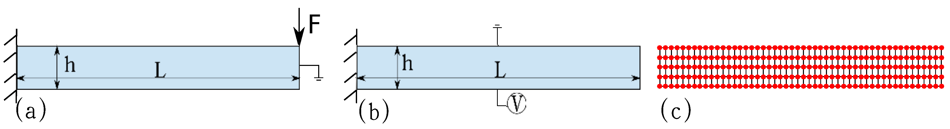
Figure 2a,b shows the simulation setup for open circuit mechanical loading and close circuit electrical loading, respectively. The length to thickness ratio for the cantilever beam is 20. Table 1 reports the various material parameters [21].
3.1.1. Mechanical Loading
A point load N is applied on the upper right edge of the cantilever beam (Figure 2a), and the electric potential is constrained to zero. Electromechanical coupling induces the electrical energy under point load deformation. The conversion from mechanical to electrical energy is defined as:
The present model is simplified by assuming that the transversal piezoelectric () and flexoelectric () components are the only non-zero in Equations (12) and (13). The Poisson effect is also ignored. The results of this simplified model are compared with the analytical model derived by Majdoub et al. [50]. The analytical solution for is:
where the normalized piezoelectric constant is:
where is obtained by neglecting flexoelectricity coefficient in Equation (15).
Figure 3a plots the comparison between the present model and the analytical solution, where is the normalized beam thickness for the open circuit mechanical loading condition. The variation between and from the present model agrees with the analytical solution from Equation (16). This proves that the present model correctly estimates the electromechanical coupling in a non-piezoelectric beam under bending deformation. The coupling between mechanical and electric energy is strongly mediated by the flexoelectricity due to the low piezoelectric constant of the material (refer to Table 1). Figure 3b shows the distribution of the generated electric potential under the flexoelectric effect.
3.1.2. Electrical Loading
In this section, we study a cantilever beam (Figure 2b) under pure electric loading, which served as an actuator. The bottom edge of the cantilever beam (Figure 2b) enforced an electrical loading of −20V and grounded the top edge. There is no external mechanical loading in the cantilever beam. Figure 4 displays the displacement and electric potential profiles. The electric field across the beam in the y-direction is plotted in Figure 5. The electric field gradients near the top (negative sign) and bottom (positive sign) surface of the cantilever beam are due to the effect of converse flexoelectricity. This phenomenon generates mechanical stress at the top and bottom surface and thus deforms the beam. The displacement and electric potential distribution on the cantilever beam are in good agreement with earlier findings based on IGA analysis [21].
3.2. Compress Truncated Pyramid
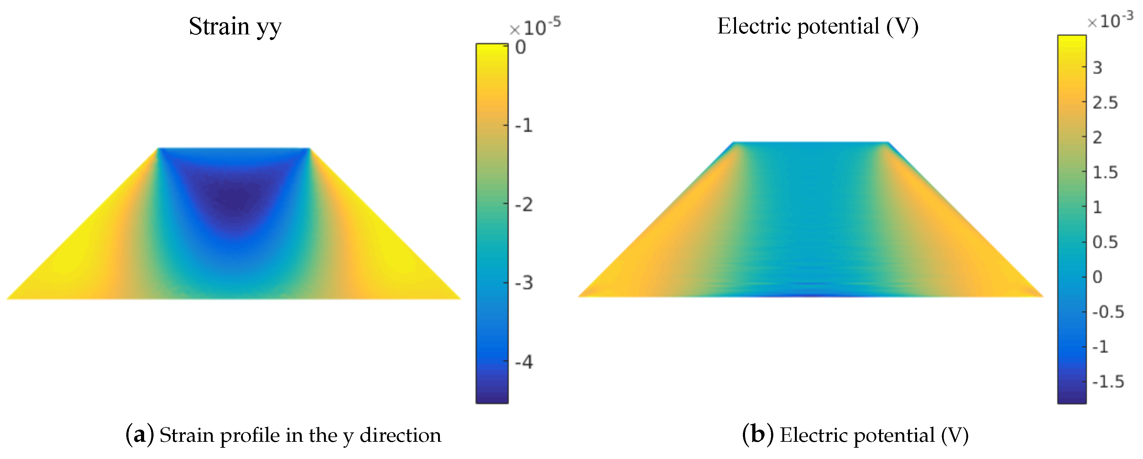
In this section, we have extended the validation for the compression of a truncated pyramid (Figure 6). Due to its different top () and bottom () edge lengths, the applied uniform force F generates different tractions at the top and bottom edges, which results in a longitudinal strain gradient. The top edge of the pyramid is grounded, and a uniform force of N is applied to it. The aspect ratio h of the pyramid is set as 75 m, and the bottom edge length is 225 m. The remaining material parameters are listed in Table 1. Figure 7 shows the developed strain in the y-direction and the electromechanical coupling-induced electric potential profiles. The numerical values and the field distributions are in good agreement with earlier reports [21]. This represents that the present model accurately estimated the electromechanical coupling.
3.3. Flexoelectricity in Composite
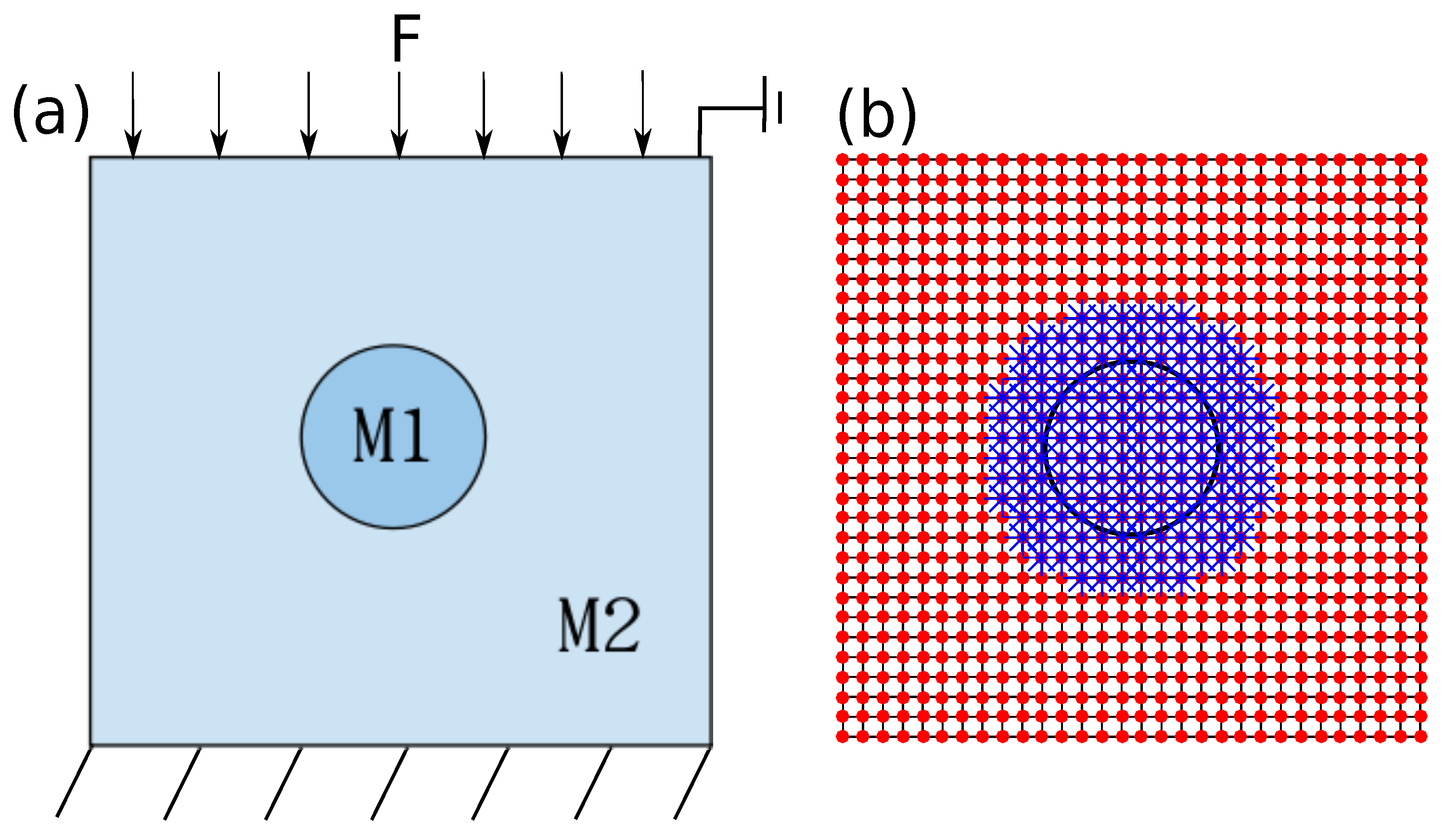
In this section, we demonstrate the possibility of inducing electric polarization in a composite system. The composite system is a combination of an embedding matrix in a square shape and a non-piezoelectric material (inclusion) in a circular shape, as shown in Figure 8. The composite under a uniform mechanical loading induces electrical polarization due to the local strain gradients near the material discontinuity. The dielectric constant of the inclusion material is about of the embedding matrix. It is assumed that the Young’s modulus of the matrix material () is lower than the Young’s modulus of the inclusion material (). Three different Young’s modulus ratios () are used to understand its influence on the energy transfer ratio between mechanical energy and electrical energy. The edge length of the square domain is L = 10 m with center inclusion radius = 1.5 m. The remaining parameters (Table 1) for both materials are similar.
Figure 9 presents the strain and electric potential profile for the domain with a center inclusion. The non-uniform strain field near the inclusion boundary generates the polarization gradient and electric potential. Figure 10 plots the strain gradient profile: and along the horizontal and vertical center line of the square domain, respectively. In both directions, a high strain gradient is seen near the boundary of the inclusion, which is due to the different material toughness of the matrix and the inclusion. Since the inclusion material is a non-piezoelectric material, the induced electrical potential is a consequence of flexoelectricity. Therefore, the linear relationship between electrical potential and strain gradient generates the strong potential near the inclusion, as seen from Figure 9b.
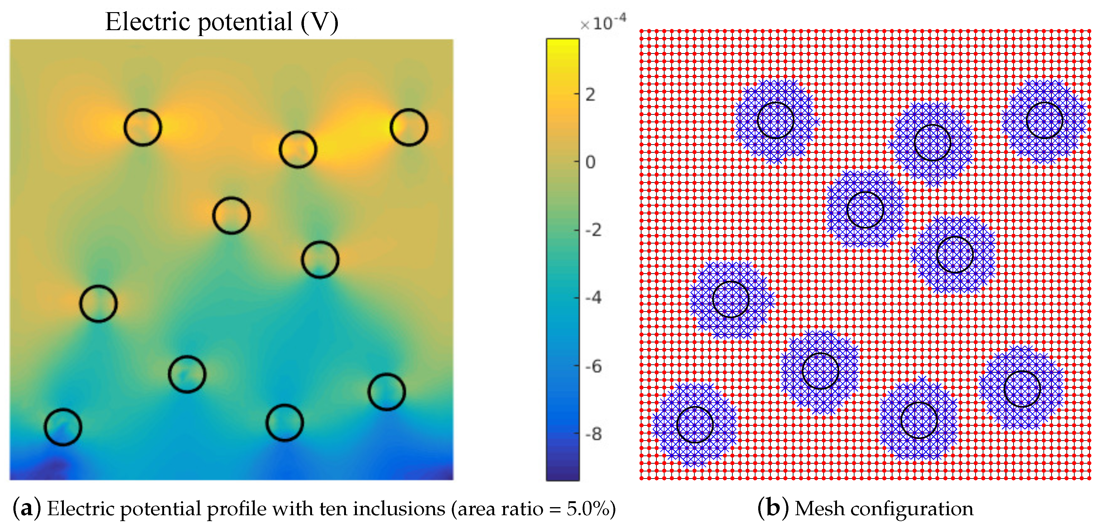
In general, the volume percentage of the inclusions has a vast impact on the overall composite properties [56]. In order to investigate the volume percentage effect on the electromechanical coupling, we have repeated the simulations with many inclusions under the same loading condition. The number of inclusions is varied according to the area ratio from –. The area ratio is defined as the total area of inclusions divided by the area of a square domain. For each area ratio, several inclusion configurations (center location for inclusions) are examined, and later, the results are averaged. Note that, for inserting many inclusions, the radius is decreased to m. Figure 11a shows the strong electric potential near the inclusion boundary for a domain with 10 randomly-distributed inclusions. This is due to the non-uniform strain distributions near the inclusion boundary. A strong electric potential is noted in the region between the nearby inclusions. This corresponds to the interaction of the non-uniform strain fields around the neighboring inclusions. Figure 11b shows the mesh configuration. Figure 12 plots the variation of the total electrical energy transfer rate with the area ratio. The energy transfer increases with the increase of the inclusion area ratio. This behavior is expected since higher irregularities of strain are induced when many inclusions are present. Figure 12 also indicates that domains with an identical inclusion area ratio with higher induce higher energy conversion from mechanical to electrical energy. This suggests that softer matrix materials enhance the electromechanical coupling characteristics.
4. Conclusions
In this study, the proposed model demonstrates the possibilities of inducing electromechanical coupling in a nano-composite material without the presence of the piezoelectric effect. The electromechanical coupling is modeled using the EFG method. Strain gradient involving partial differential equations is numerically solved using the MLS approximation. The continuity due to the strain gradient term is fulfilled by choosing the special weight function in the EFG. The level set techniques are employed to handle the weak discontinuity between the inclusion and matrix. The present numerical model captures the finite size flexoelectric effect for a mechanically-loaded cantilever beam. The converse flexoelectric effect-induced mechanical deformation of an electrically loaded cantilever beam is in good agreement with earlier reports. The results of the truncated pyramid further validate the current model. The non-uniform strain fields near the inclusion boundary induce the electrical polarization and thus electric potential due to flexoelectricity. We also found that the magnitude of the electromechanical coupling is largely dependent on the area ratio between the inclusion and the matrix. The higher the inclusion area ratio, the stronger the electromechanical coupling. Furthermore, a softer matrix material can also enhance the electromechanical coupling when compared to a stiff material. These findings help in designing a nano-composite utilizing the flexoelectric effect.
Author Contributions
Conceptualization, B.H.; Methodology, B.H.; Software, B.H.; Validation, B.H.; Formal Analysis, B.H. and B.J.; Investigation, B.H. and B.J.; Resources, B.H. and B.J.; Data Curation, B.H. and B.J.; Writing-Original Draft Preparation, B.H. and B.J.; Writing-Review and Editing, B.H. and B.J.; Visualization, B.H. and B.J.; Supervision, X.Z.; Project Administration, X.Z.; Funding Acquisition, X.Z.
Funding
This research is funded by the National Science Foundation of China (11772234) and ERC Starting Grant 802205.
Conflicts of Interest
Authors declare no conflict of interest.
Appendix A. Theory of Flexoelectricity
The enthalpy density for a dielectric solid with piezoelectric and flexoelectric effects is [50,51]:
where is the electric field; is the electric potential; is the mechanical strain; is the fourth-order elastic moduli tensor; is the third-order tensor of piezoelectricity; and are the fourth-order direct and converse flexoelectric tensors; and is the second-order dielectric tensor. Sharma et al. [52] defined the flexoelectric tensor as the difference between and by the application of integration by parts and Gauss divergence theorem to Equation (A1), which is:
The stress and electric displacement from Equation (1) when considering the piezoelectricity effect is given as:
Due to the presence of flexoelectricity, the higher-order stress and electric displacement read:
The total stress and electric displacement from piezoelectric and flexoelectric effects are summarized as:
The essential and natural electric boundary condition are:
where and w are the applied electric potential and surface charge density, represents the boundary of the domain, and is the unit normal to the boundary . The mechanical boundary conditions are given as:
where and are prescribed mechanical displacement and traction. The remaining boundary conditions (normal derivation of displacement and higher-order tractions) resulting from the strain gradient have been set to zero under the assumption of a homogeneous condition.
Rewrite Equations (A3) and (A4) as:
and integration over the domain gives:
where is the total electrical enthalpy. The external work by surface mechanical and electrical forces is given by:
Finally, the weak form of the mechanical and electrical equilibrium derived from the Hamilton principle for the static problem yields:
The unknowns (displacement and electric potential) in Equation (A12) are approximated using MLS.
Appendix B. Details of the Shape Function
The shape function associates with Node I and a point x under MLS is:
where is the second-order polynomial, which is:
The quadratic spline weight function w ensures continuity inside an element and continuity between elements [40]. The mathematical expression for w is:
where:
d is the predefined search radius of the support domain and d equals three-times the nodal spacing. The moment matrix has the form:
A sufficient number of support nodes ensures the non-singularity of matrix . The enrichment function has the form [42]:
where is the total number of inclusions inside the domain, is the center coordinate of the circular inclusion, and is the radius of the circular inclusion.
Appendix C. Mathematical Expression for the Elements in Equation (4)
References
- Chen, J.; Qiu, Q.; Han, Y.; Lau, D. Piezoelectric materials for sustainable building structures: Fundamentals and applications. Renew. Sustain. Energy Rev. 2019, 101, 14–25. [Google Scholar] [CrossRef]
- Cabeza, L.F.; Barreneche, C.; Miró, L.; Morera, J.M.; Bartolí, E.; Fernández, A.I. Low carbon and low embodied energy materials in buildings: A review. Renew. Sustain. Energy Rev. 2013, 23, 536–542. [Google Scholar] [CrossRef]
- Ramesh, T.; Prakash, R.; Shukla, K. Life cycle energy analysis of buildings: An overview. Energy Build. 2010, 42, 1592–1600. [Google Scholar] [CrossRef]
- Scopelianos, A.G. Piezoelectric Biomedical Device. US Patent 5,522,879, 4 June 1996. [Google Scholar]
- Zhou, Q.; Lau, S.; Wu, D.; Shung, K.K. Piezoelectric films for high frequency ultrasonic transducers in biomedical applications. Prog. Mater. Sci. 2011, 56, 139–174. [Google Scholar] [CrossRef] [PubMed] [Green Version]
- Jiang, X.; Huang, W.; Zhang, S. Flexoelectric nano-generator: Materials, structures and devices. Nano Energy 2013, 2, 1079–1092. [Google Scholar] [CrossRef]
- Zhuang, X.Y.; Huang, R.Q.; Liang, C.; Rabczuk, T. A coupled thermo-hydro-mechanical model of jointed hard rock for compressed air energy storage. Math. Probl. Eng. 2014, 2014, 179169. [Google Scholar] [CrossRef]
- Ahmadpoor, F.; Sharma, P. Flexoelectricity in two-dimensional crystalline and biological membranes. Nanoscale 2015, 7, 16555–16570. [Google Scholar] [CrossRef]
- Ma, W.; Cross, L.E. Observation of the flexoelectric effect in relaxor Pb (Mg 1/3 Nb 2/3) O 3 ceramics. Appl. Phys. Lett. 2001, 78, 2920–2921. [Google Scholar] [CrossRef]
- Ma, W.; Cross, L.E. Flexoelectricity of barium titanate. Appl. Phys. Lett. 2006, 88, 232902. [Google Scholar] [CrossRef]
- Hong, J.; Catalan, G.; Scott, J.; Artacho, E. The flexoelectricity of barium and strontium titanates from first principles. J. Phys. Condens. Matter 2010, 22, 112201. [Google Scholar] [CrossRef] [Green Version]
- Xu, T.; Wang, J.; Shimada, T.; Kitamura, T. Direct approach for flexoelectricity from first-principles calculations: Cases for SrTiO3 and BaTiO3. J. Phys. Condens. Matter 2013, 25, 415901. [Google Scholar] [CrossRef] [PubMed]
- Kundalwal, S.; Meguid, S.; Weng, G. Strain gradient polarization in graphene. Carbon 2017, 117, 462–472. [Google Scholar] [CrossRef]
- Javvaji, B.; He, B.; Zhuang, X. The generation of piezoelectricity and flexoelectricity in graphene by breaking the materials symmetries. Nanotechnology 2018, 29, 225702. [Google Scholar] [CrossRef] [PubMed] [Green Version]
- He, B.; Javvaji, B.; Zhuang, X. Size dependent flexoelectric and mechanical properties of barium titanate nanobelt: A molecular dynamics study. Phys. B Condens. Matter 2018, 545, 527–535. [Google Scholar] [CrossRef]
- Zhang, Z.; Geng, D.; Wang, X. Calculation of the piezoelectric and flexoelectric effects in nanowires using a decoupled finite element analysis method. J. Appl. Phys. 2016, 119, 154104. [Google Scholar] [CrossRef] [Green Version]
- Nanthakumar, S.; Zhuang, X.; Park, H.S.; Rabczuk, T. Topology optimization of flexoelectric structures. J. Mech. Phys. Solids 2017, 105, 217–234. [Google Scholar] [CrossRef]
- Nanthakumar, S.S.; Lahmer, T.; Zhuang, X.Y.; Zi, G.; Rabczuk, T. Detection of material interfaces using a regularized level set method in piezoelectric structures. Inverse Probl. Sci. Eng. 2016, 24, 153–176. [Google Scholar] [CrossRef]
- Deng, F.; Deng, Q.; Yu, W.; Shen, S. Mixed Finite Elements for Flexoelectric Solids. J. Appl. Mech. 2017, 84, 081004. [Google Scholar] [CrossRef]
- Mao, S.; Purohit, P.K.; Aravas, N. Mixed finite-element formulations in piezoelectricity and flexoelectricity. Proc. R. Soc. A 2016, 472, 20150879. [Google Scholar] [CrossRef] [Green Version]
- Ghasemi, H.; Park, H.S.; Rabczuk, T. A level-set based IGA formulation for topology optimization of flexoelectric materials. Comput. Methods Appl. Mech. Eng. 2017, 313, 239–258. [Google Scholar] [CrossRef]
- Hamdia, K.M.; Ghasemi, H.; Zhuang, X.Y.; Alajlan, N.; Rabczuk, T. Sensitivity and uncertainty analysis for flexoelectric nanostructures. Comput. Methods Appl. Mech. Eng. 2018, 337, 95–109. [Google Scholar] [CrossRef]
- Nguyen-Thanh, N.; Valizadeh, N.; Nguyen, M.N.; Nguyen-Xuan, H.; Zhuang, X.Y.; Areias, P.; Zi, G.; Bazilevs, Y.; De Lorenzis, L.; Rabczuk, T. An extended isogeometric thin shell analysis based on Kirchhoff–Love theory. Comput. Methods Appl. Mech. Eng. 2015, 284, 265–291. [Google Scholar] [CrossRef]
- Nguyen, V.P.; Anitescu, C.; Bordas, S.P.; Rabczuk, T. Isogeometric analysis: An overview and computer implementation aspects. Math. Comput. Simul. 2015, 117, 89–116. [Google Scholar] [CrossRef] [Green Version]
- Hughes, T.J.; Cottrell, J.A.; Bazilevs, Y. Isogeometric analysis: CAD, finite elements, NURBS, exact geometry and mesh refinement. Comput. Methods Appl. Mech. Eng. 2005, 194, 4135–4195. [Google Scholar] [CrossRef]
- Abdollahi, A.; Peco, C.; Millán, D.; Arroyo, M.; Arias, I. Computational evaluation of the flexoelectric effect in dielectric solids. J. Appl. Phys. 2014, 116, 093502. [Google Scholar] [CrossRef]
- Abdollahi, A.; Millán, D.; Peco, C.; Arroyo, M.; Arias, I. Revisiting pyramid compression to quantify flexoelectricity: A three-dimensional simulation study. Phys. Rev. B 2015, 91, 104103. [Google Scholar] [CrossRef]
- Bernholc, J.; Nakhmanson, S.M.; Nardelli, M.B.; Meunier, V. Understanding and enhancing polarization in complex materials. Comput. Sci. Eng. 2004, 6, 12–21. [Google Scholar] [CrossRef] [Green Version]
- Ghidelli, M.; Sebastiani, M.; Collet, C.; Guillemet, R. Determination of the elastic moduli and residual stresses of freestanding Au-TiW bilayer thin films by nanoindentation. Mater. Des. 2016, 106, 436–445. [Google Scholar] [CrossRef]
- Msekh, M.A.; Cuong, N.H.; Zi, G.; Areias, P.; Zhuang, X.Y.; Rabczuk, T. Fracture properties prediction of clay/epoxy nanocomposites with interphase zones using a phase field model. Eng. Fract. Mech. 2018, 188, 287–299. [Google Scholar] [CrossRef]
- Bhavanasi, V.; Kumar, V.; Parida, K.; Wang, J.; Lee, P.S. Enhanced Piezoelectric Energy Harvesting Performance of Flexible PVDF-TrFE Bilayer Films with Graphene Oxide. ACS Appl. Mater. Interfaces 2016, 8, 521–529. [Google Scholar] [CrossRef]
- Biswal, A.K.; Das, S.; Roy, A. Designing and synthesis of a polymer matrix piezoelectric composite for energy harvesting. IOP Conf. Ser. Mater. Sci. Eng. 2017, 178, 012002. [Google Scholar] [CrossRef] [Green Version]
- Sidhardh, S.; Ray, M.C. Effective properties of flexoelectric fiber-reinforced nanocomposite. Mater. Today Commun. 2018, 17, 114–123. [Google Scholar] [CrossRef]
- Hamdia, K.M.; Silani, M.; Zhuang, X.Y.; He, P.F.; Rabczuk, T. Stochastic analysis of the fracture toughness of polymeric nanoparticle composites using polynomial chaos expansions. Int. J. Fract. 2017, 206, 215–227. [Google Scholar] [CrossRef]
- Ghasemi, H.; Park, H.S.; Rabczuk, T. A multi-material level set-based topology optimization of flexoelectric composites. Comput. Methods Appl. Mech. Eng. 2018, 332, 47–62. [Google Scholar] [CrossRef]
- Cordes, L.; Moran, B. Treatment of material discontinuity in the element-free Galerkin method. Comput. Methods Appl. Mech. Eng. 1996, 139, 75–89. [Google Scholar] [CrossRef]
- Rabczuk, T.; Belytschko, T.; Xiao, S.P. Stable particle methods based on Lagrangian kernels. Comput. Methods Appl. Mech. Eng. 2004, 193, 1035–1063. [Google Scholar] [CrossRef]
- Krongauz, Y.; Belytschko, T. EFG approximation with discontinuous derivatives. Int. J. Numer. Methods Eng. 1998, 41, 1215–1233. [Google Scholar] [CrossRef]
- Rabczuk, T.; Zi, G.; Bordas, S.; Nguyen-Xuan, H. A geometrically non-linear three-dimensional cohesive crack method for reinforced concrete structures. Eng. Fract. Mech. 2008, 75, 4740–4758. [Google Scholar] [CrossRef] [Green Version]
- Nguyen, V.P.; Rabczuk, T.; Bordas, S.; Duflot, M. Meshless methods: A review and computer implementation aspects. Math. Comput. Simul. 2008, 79, 763–813. [Google Scholar] [CrossRef] [Green Version]
- Budarapu, P.R.; Gracie, R.; Yang, S.W.; Zhuang, X.Y.; Rabczuk, T. Efficient coarse graining in multiscale modeling of fracture. Theor. Appl. Fract. Mech. 2014, 69, 126–143. [Google Scholar] [CrossRef]
- Sukumar, N.; Chopp, D.L.; Moës, N.; Belytschko, T. Modeling holes and inclusions by level sets in the extended finite-element method. Comput. Methods Appl. Mech. Eng. 2001, 190, 6183–6200. [Google Scholar] [CrossRef] [Green Version]
- Ren, H.L.; Zhuang, X.Y.; Rabczuk, T. Dual-horizon peridynamics: A stable solution to varying horizons. Comput. Methods Appl. Mech. Eng. 2017, 318, 762–782. [Google Scholar] [CrossRef] [Green Version]
- Ren, H.L.; Zhuang, X.Y.; Cai, Y.C.; Rabczuk, T. Dual-horizon peridynamics. Int. J. Numer. Methods Eng. 2016, 108, 1451–1476. [Google Scholar] [CrossRef] [Green Version]
- Rabczuk, T.; Bordas, S.; Zi, G. On three-dimensional modelling of crack growth using partition of unity methods. Comput. Struct. 2010, 88, 1391–1411. [Google Scholar] [CrossRef]
- Rabczuk, T.; Areias, P.M.A.; Belytschko, T. A meshfree thin shell method for non-linear dynamic fracture. Int. J. Numer. Methods Eng. 2007, 72, 524–548. [Google Scholar] [CrossRef] [Green Version]
- Rabczuk, T.; Belytschko, T. A three-dimensional large deformation meshfree method for arbitrary evolving cracks. Comput. Methods Appl. Mech. Eng. 2007, 196, 2777–2799. [Google Scholar] [CrossRef] [Green Version]
- Rabczuk, T.; Belytschko, T. Cracking particles: A simplified meshfree method for arbitrary evolving cracks. Int. J. Numer. Methods Eng. 2004, 61, 2316–2343. [Google Scholar] [CrossRef]
- Rabczuk, T.; Bordas, S.; Zi, G. A three-dimensional meshfree method for continuous multiple-crack initiation, propagation and junction in statics and dynamics. Comput. Mech. 2007, 40, 473–495. [Google Scholar] [CrossRef] [Green Version]
- Majdoub, M.; Sharma, P.; Cagin, T. Enhanced size-dependent piezoelectricity and elasticity in nanostructures due to the flexoelectric effect. Phys. Rev. B 2008, 77, 125424. [Google Scholar] [CrossRef]
- Majdoub, M.S.; Sharma, P.; Çağin, T. Erratum: Enhanced size-dependent piezoelectricity and elasticity in nanostructures due to the flexoelectric effect [Phys. Rev. B 77, 125424 (2008)]. Phys. Rev. B 2009, 79, 119904. [Google Scholar] [CrossRef]
- Sharma, N.; Landis, C.; Sharma, P. Piezoelectric thin-film superlattices without using piezoelectric materials. J. Appl. Phys. 2010, 108, 024304. [Google Scholar] [CrossRef] [Green Version]
- Belytschko, T.; Lu, Y.Y.; Gu, L. Element-free Galerkin methods. Int. J. Numer. Methods Eng. 1994, 37, 229–256. [Google Scholar] [CrossRef]
- Belytschko, T.; Lu, Y.; Gu, L.; Tabbara, M. Element-free Galerkin methods for static and dynamic fracture. Int. J. Solids Struct. 1995, 32, 2547–2570. [Google Scholar] [CrossRef]
- Belytschko, T.; Black, T. Elastic crack growth in finite elements with minimal remeshing. Int. J. Numer. Methods Eng. 1999, 45, 601–620. [Google Scholar] [CrossRef]
- He, B.; Mortazavi, B.; Zhuang, X.; Rabczuk, T. Modeling Kapitza resistance of two-phase composite material. Compos. Struct. 2016, 152, 939–946. [Google Scholar] [CrossRef]
Figure 1.
Level-set function and its derivation cross the interface.

Figure 2.
Schematic illustration of the cantilever beam under (a) mechanical loading and (b) electrical loading. (c) MLS discretization with the red solid point representing the nodes.
Figure 2.
Schematic illustration of the cantilever beam under (a) mechanical loading and (b) electrical loading. (c) MLS discretization with the red solid point representing the nodes.

Figure 3.
Calculation results of the (a) size-dependent effective piezoelectric constant and (b) the electric potential profile for a fully-coupled cantilever beam.
Figure 3.
Calculation results of the (a) size-dependent effective piezoelectric constant and (b) the electric potential profile for a fully-coupled cantilever beam.

Figure 4.
Calculation result of the cantilever beam under electric loading: (a) beam displacement; (b) electric potential profile.
Figure 4.
Calculation result of the cantilever beam under electric loading: (a) beam displacement; (b) electric potential profile.

Figure 5.
Calculation result of the electric field profile across the beam in the y direction at the mid-length of the beam.
Figure 5.
Calculation result of the electric field profile across the beam in the y direction at the mid-length of the beam.
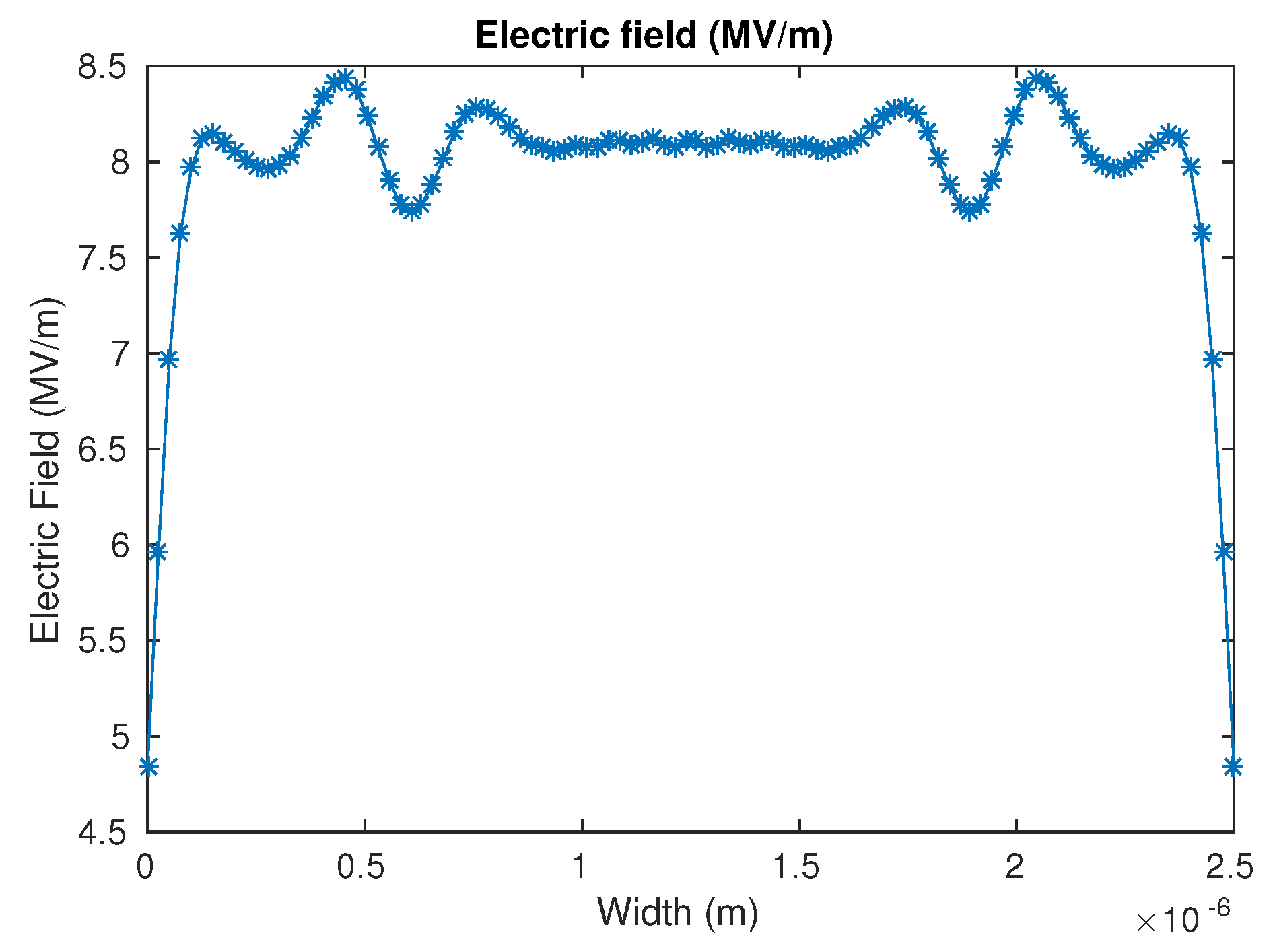
Figure 6.
Schematic illustration of: (a) the pyramid case and its boundary condition; (b) MLS discretization with the red solid point representing the nodes.
Figure 6.
Schematic illustration of: (a) the pyramid case and its boundary condition; (b) MLS discretization with the red solid point representing the nodes.
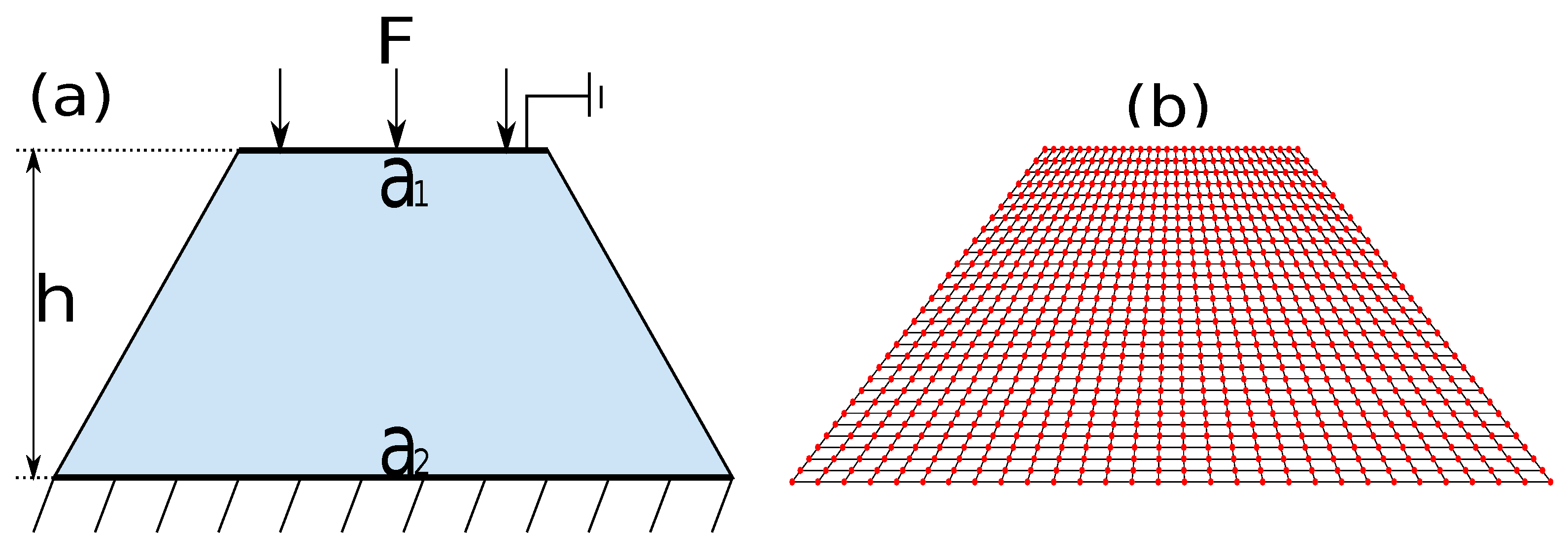
Figure 7.
Calculation result of the compressed truncated pyramid: (a) strain profile in the y direction; (b) electric field profile.
Figure 7.
Calculation result of the compressed truncated pyramid: (a) strain profile in the y direction; (b) electric field profile.

Figure 8.
Schematic illustration of: (a) the square domain with center inclusion and its boundary condition; (b) MLS discretization with the red solid point representing the nodes and the blue asterisk representing the enriched nodes.
Figure 8.
Schematic illustration of: (a) the square domain with center inclusion and its boundary condition; (b) MLS discretization with the red solid point representing the nodes and the blue asterisk representing the enriched nodes.

Figure 9.
Calculation results of a square composition under compression: (a) strain profile in the y direction; (b) induced electric potential.
Figure 9.
Calculation results of a square composition under compression: (a) strain profile in the y direction; (b) induced electric potential.
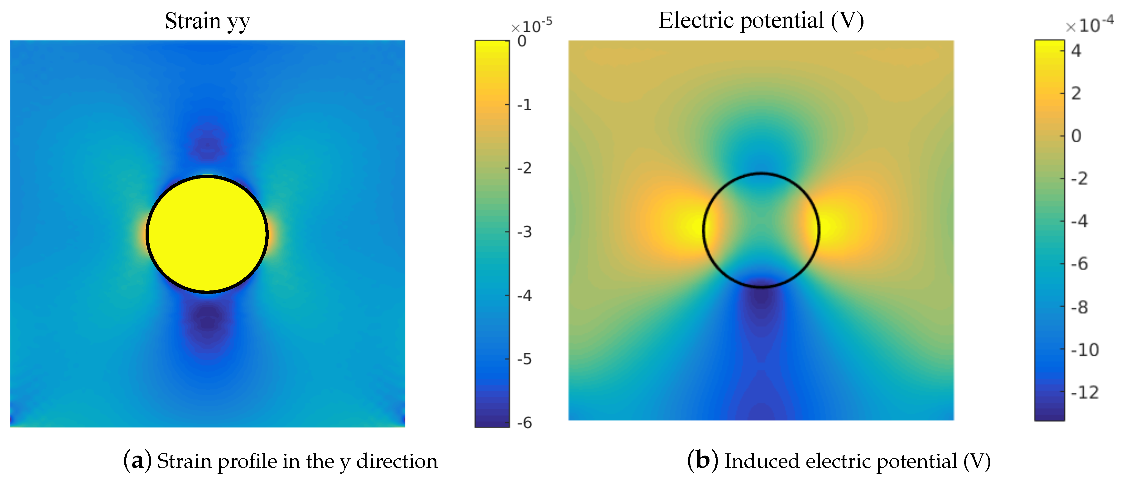
Figure 10.
Strain gradient profile at the horizontal center line () and the vertical center line ().
Figure 10.
Strain gradient profile at the horizontal center line () and the vertical center line ().
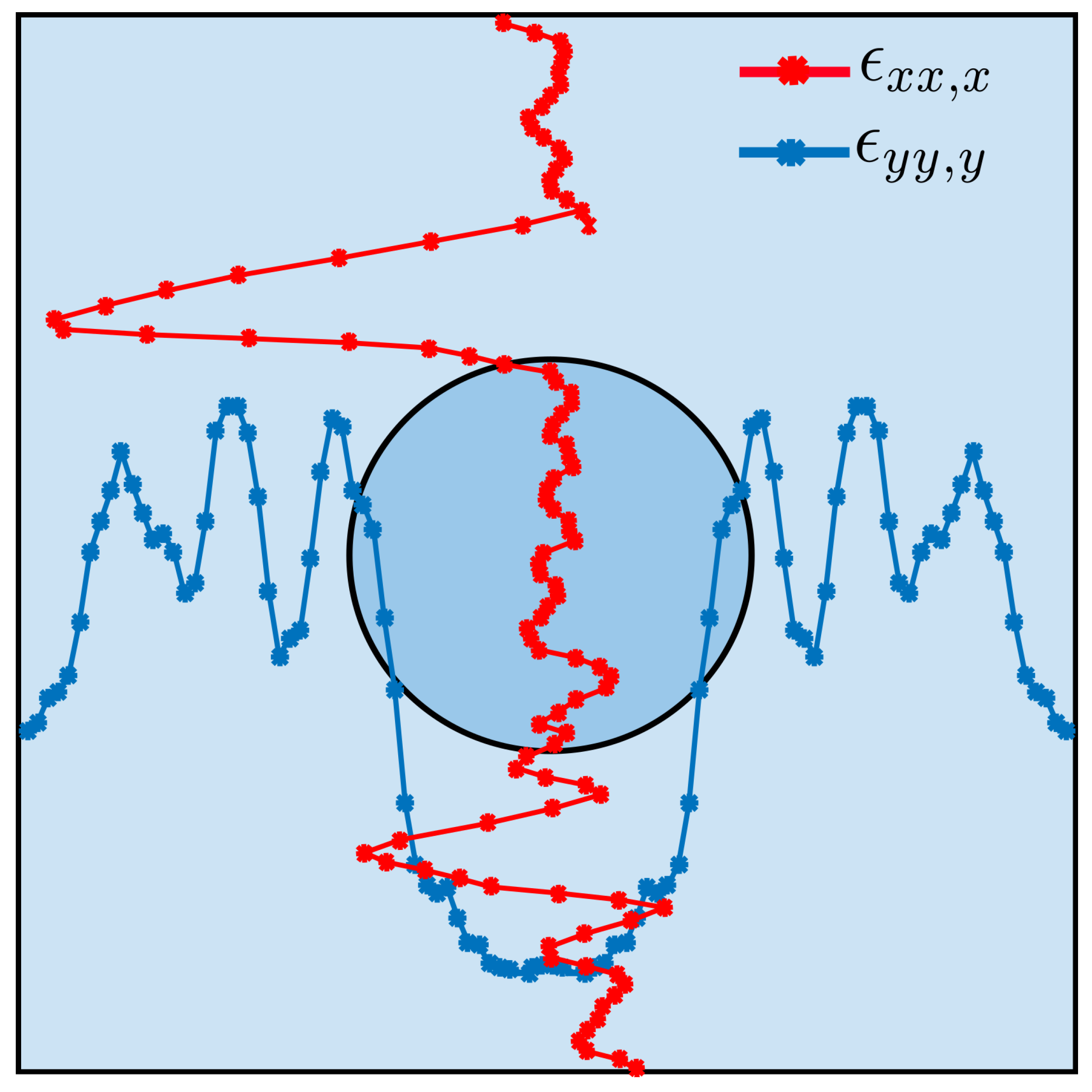
Figure 11.
Calculation results of the square domain with randomly-distributed inclusions under compression: (a) electric potential profile for the domain with ten inclusions; (b) MLS discretization with the red solid point representing the nodes and the blue asterisk representing the enriched nodes.

Figure 12.
The energy conversion rate calculated by (Equation (14)) vs. the inclusion area ratio. Several setups are created for each configuration; hereafter, the averaged results are plotted. The error bar represents the upper and lower boundary of the calculation results.
Figure 12.
The energy conversion rate calculated by (Equation (14)) vs. the inclusion area ratio. Several setups are created for each configuration; hereafter, the averaged results are plotted. The error bar represents the upper and lower boundary of the calculation results.


Table 1.
Material properties.
| Name | Symbol | Value |
|---|---|---|
| Poisson’s ratio | 0.37 | |
| Young’s modulus | E | 100 GPa |
| Piezoelectric constant | −4.4 nC/m | |
| Flexoelectric constant | 1 C/m | |
| Dielectric constant | ; | 11 nC/Vm; 12.48 nC/Vm |
| Electric susceptibility | 1408 |
© 2019 by the authors. Licensee MDPI, Basel, Switzerland. This article is an open access article distributed under the terms and conditions of the Creative Commons Attribution (CC BY) license (http://creativecommons.org/licenses/by/4.0/).
Share and Cite
MDPI and ACS Style
He, B.; Javvaji, B.; Zhuang, X. Characterizing Flexoelectricity in Composite Material Using the Element-Free Galerkin Method. Energies 2019, 12, 271. https://doi.org/10.3390/en12020271
AMA Style
He B, Javvaji B, Zhuang X. Characterizing Flexoelectricity in Composite Material Using the Element-Free Galerkin Method. Energies. 2019; 12(2):271. https://doi.org/10.3390/en12020271
Chicago/Turabian StyleHe, Bo, Brahmanandam Javvaji, and Xiaoying Zhuang. 2019. "Characterizing Flexoelectricity in Composite Material Using the Element-Free Galerkin Method" Energies 12, no. 2: 271. https://doi.org/10.3390/en12020271
Note that from the first issue of 2016, this journal uses article numbers instead of page numbers. See further details here.