Table A1.
Technical parameters of the battery and inverter system used for this study.
| Parameter | Value |
|---|
| Battery type | muRata Fortelion (Sony US26650FTC1) |
| Cathode chemistry | Lithium-iron-phosphate |
| Nominal cell voltage | 3.2 V |
| Nominal cell capacity | 3 Ah |
| Storage capacity | 36 kWh |
| Operation limits | [10 ⋯ 95] % SOC |
| Ageing model | Empirical cycle ageing model |
| Inverter type | Siemens Sinamics s120 |
| Inverter power rating | 36 kW (nominal) 43.2 kW (maximum) |
Table A2.
Optimisation parameters.
| Parameter | Value | Unit |
|---|
| 500 or 250 | EUR/kWh |
| (for ) or (for ) | EUR/ |
| 0.8 | N.A. |
| 36 | kWh |
| 36 | kW |
| 43.2 | kW |
| 0.95 | N.A. |
| 0.1 | N.A. |
| (IDM) or (DAM) | N.A. |
| 0.25 (IDM) or 1 hour (DAM) | h |
| , | 1 | N.A. |
| −3.18 | |
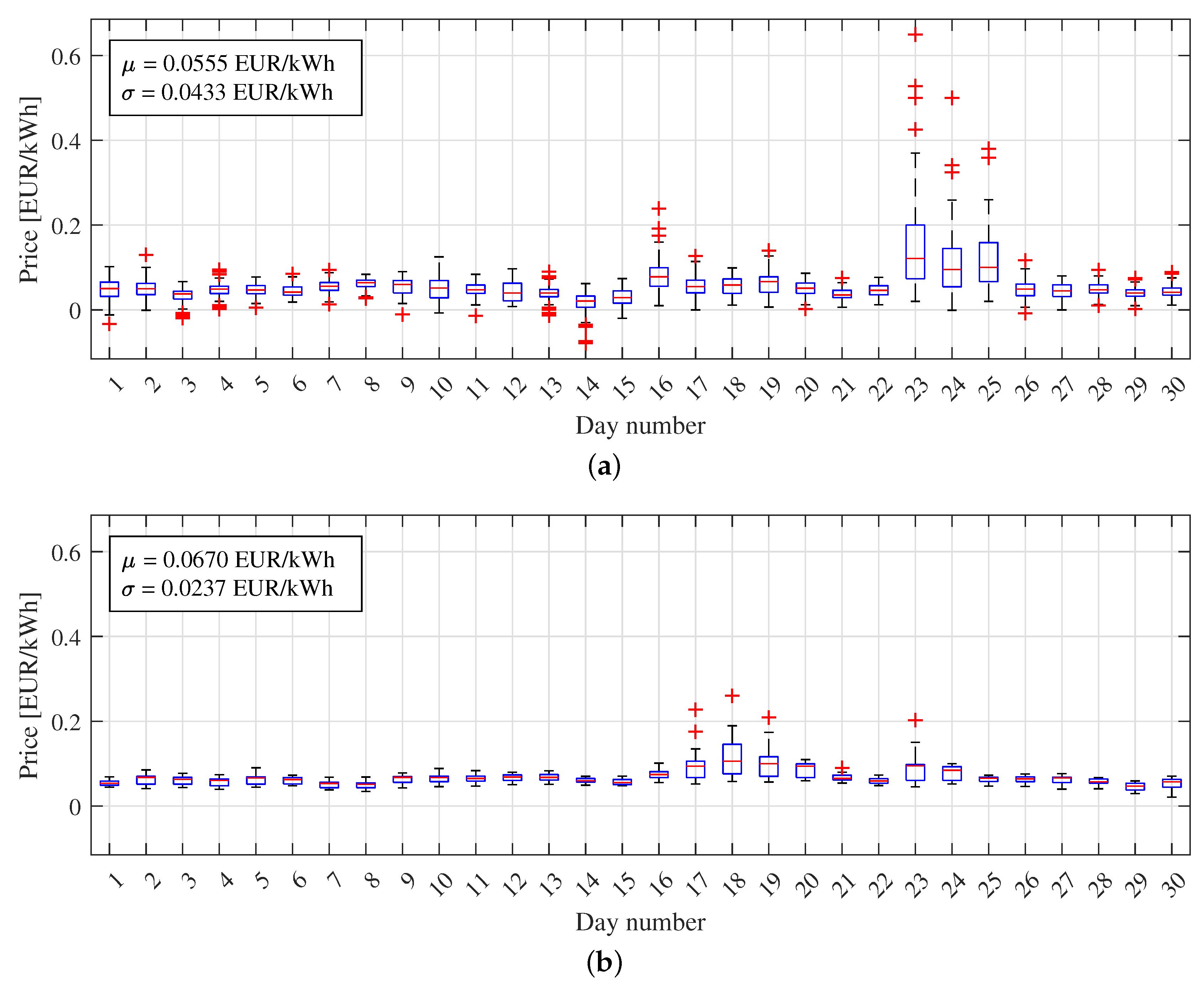
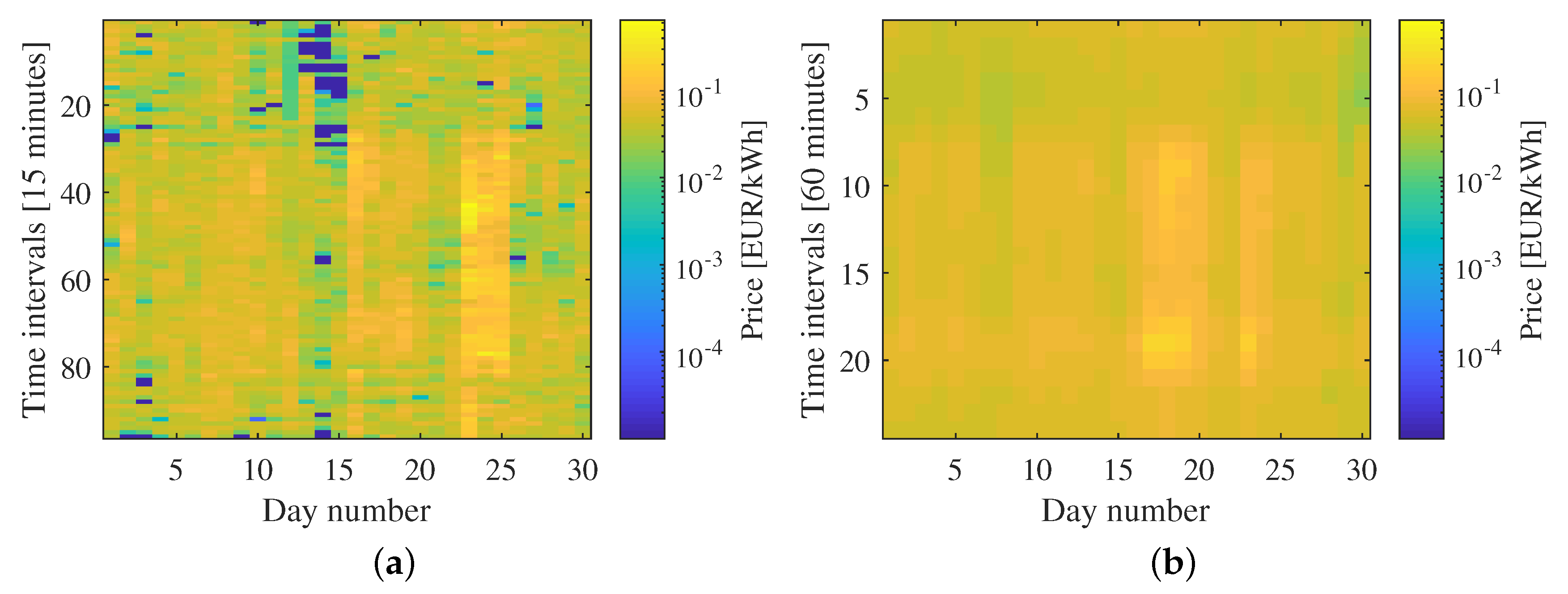
Figure A1.
Price distribution for (a) the intraday market; and (b) the day-ahead market.
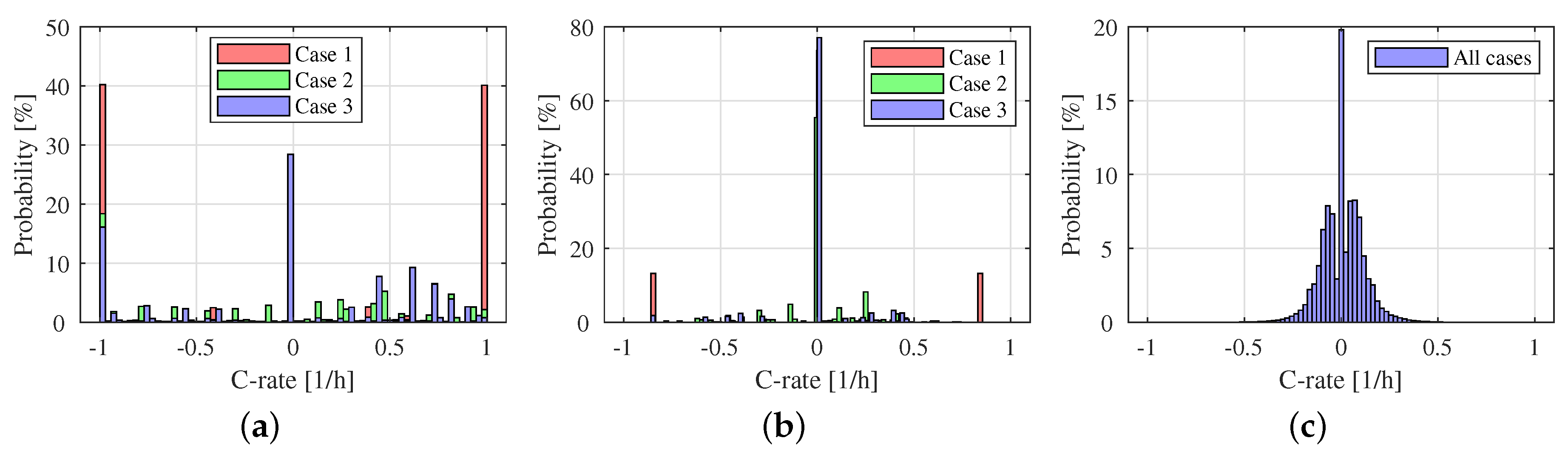
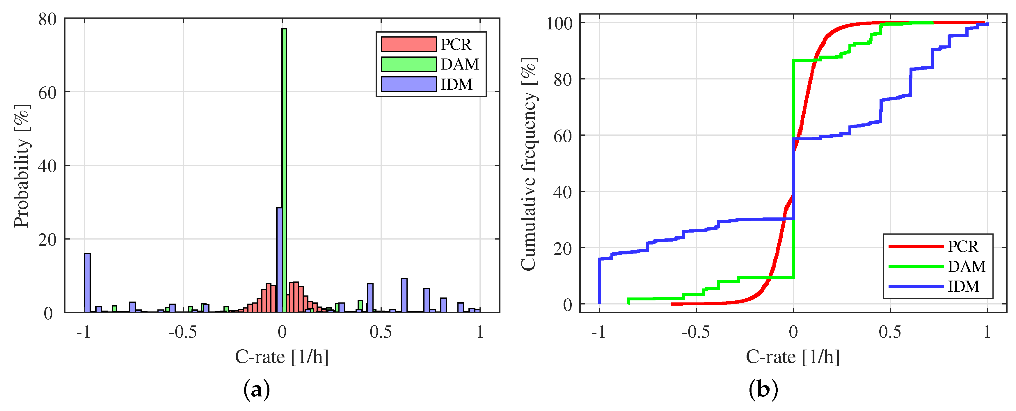
Figure A2.
Histogram plots of C-rate for (a) the intraday market; (b) the day-ahead market; and (c) the primary control reserve.
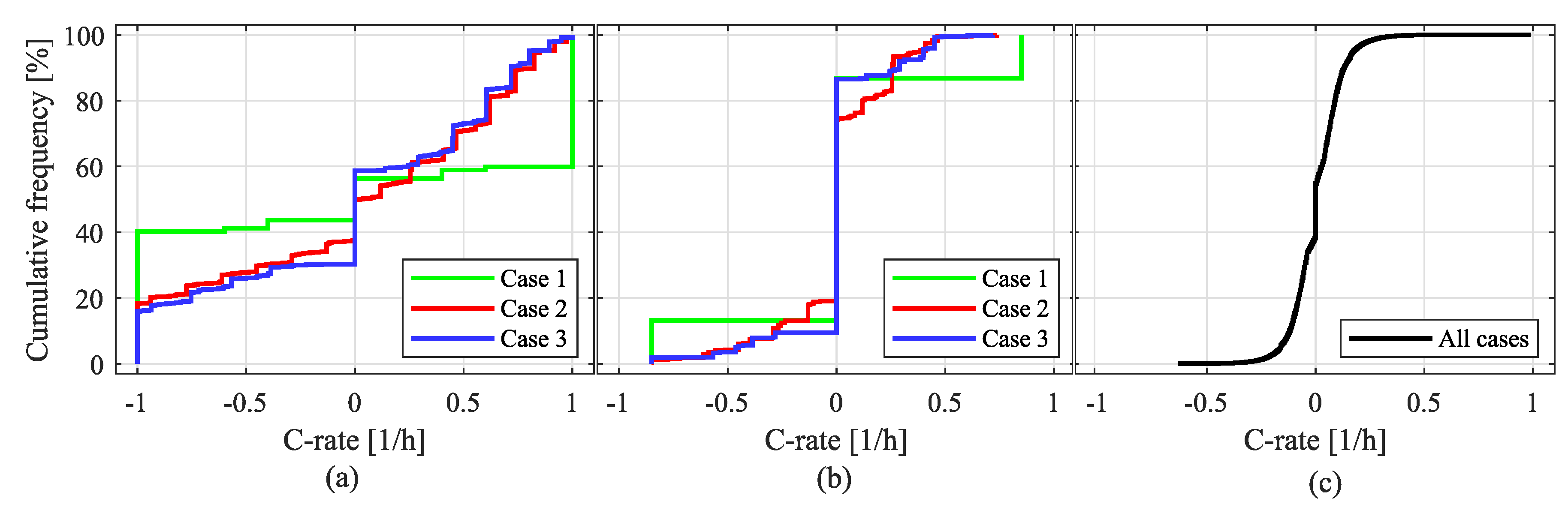
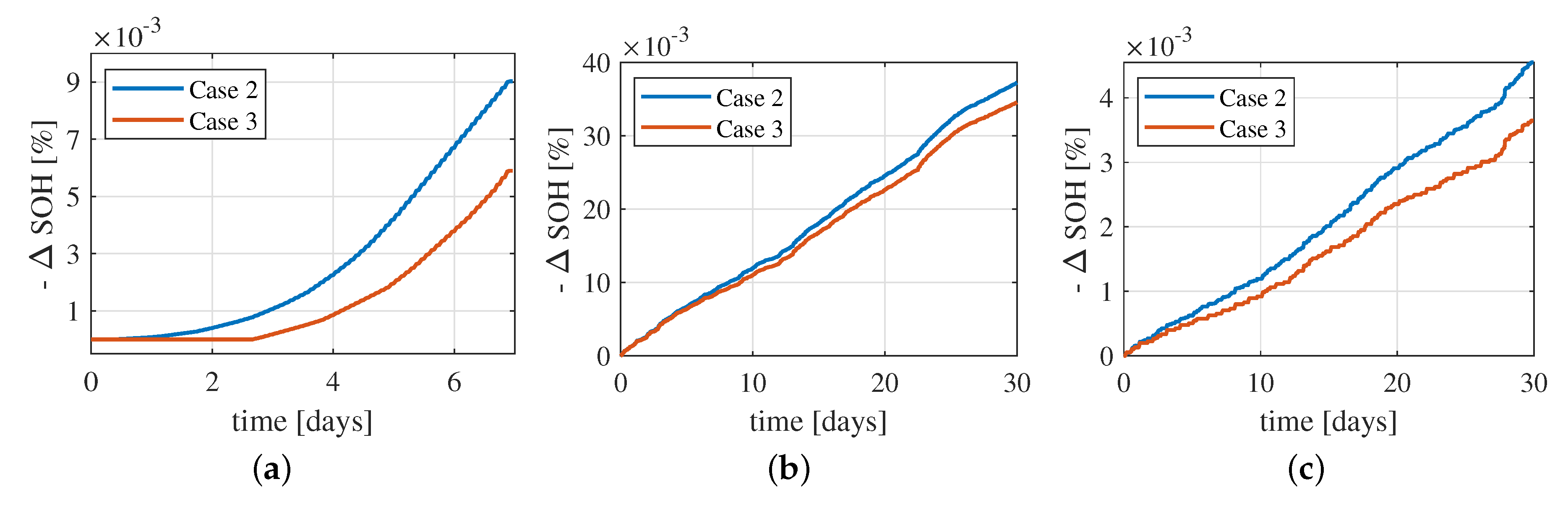
Figure A3.
For PCR, DAM, and IDM in the Case 3 scenario (considering all losses and ageing): (a) Histogram plots; and (b) cumulative distribution.
Table A3.
Table of efficiencies concerning real-world data.
| Application and Dataset | System Indicators under Different Cases |
|---|
| Case 1 | Case 2 | Case 3 |
|---|
| Battery Cost (per kWh) | | 250 EUR | 500 EUR | 250 EUR | 500 EUR |
|---|
| Intraday Market | | | | | |
| Energy throughput [kWh] | 21,647 | 16,073 | 14,498 | 14,461 | 12,924 |
| Full equivalent cycle [-] | 301 | 223 | 201 | 201 | 180 |
| Mean round-trip efficiency [%] | 100 | 93.3 | 93.6 | 88.7 | 89.0 |
| Day Ahead Market | | | | | |
| Energy throughput [kWh] | 5814 | 3656 | 3418 | 2721 | 2487 |
| Full equivalent cycle [-] | 81 | 51 | 47 | 38 | 35 |
| Mean round-trip efficiency [%] | 100 | 96.6 | 96.7 | 90.6 | 90.6 |
| PCR (Reference Operation) | | | | | |
| Energy throughput [kWh] | – | – | – | 2168 |
| Full equivalent cycle [-] | – | – | – | 28 |
| Mean round-trip efficiency [%] | – | – | – | 80.7 |
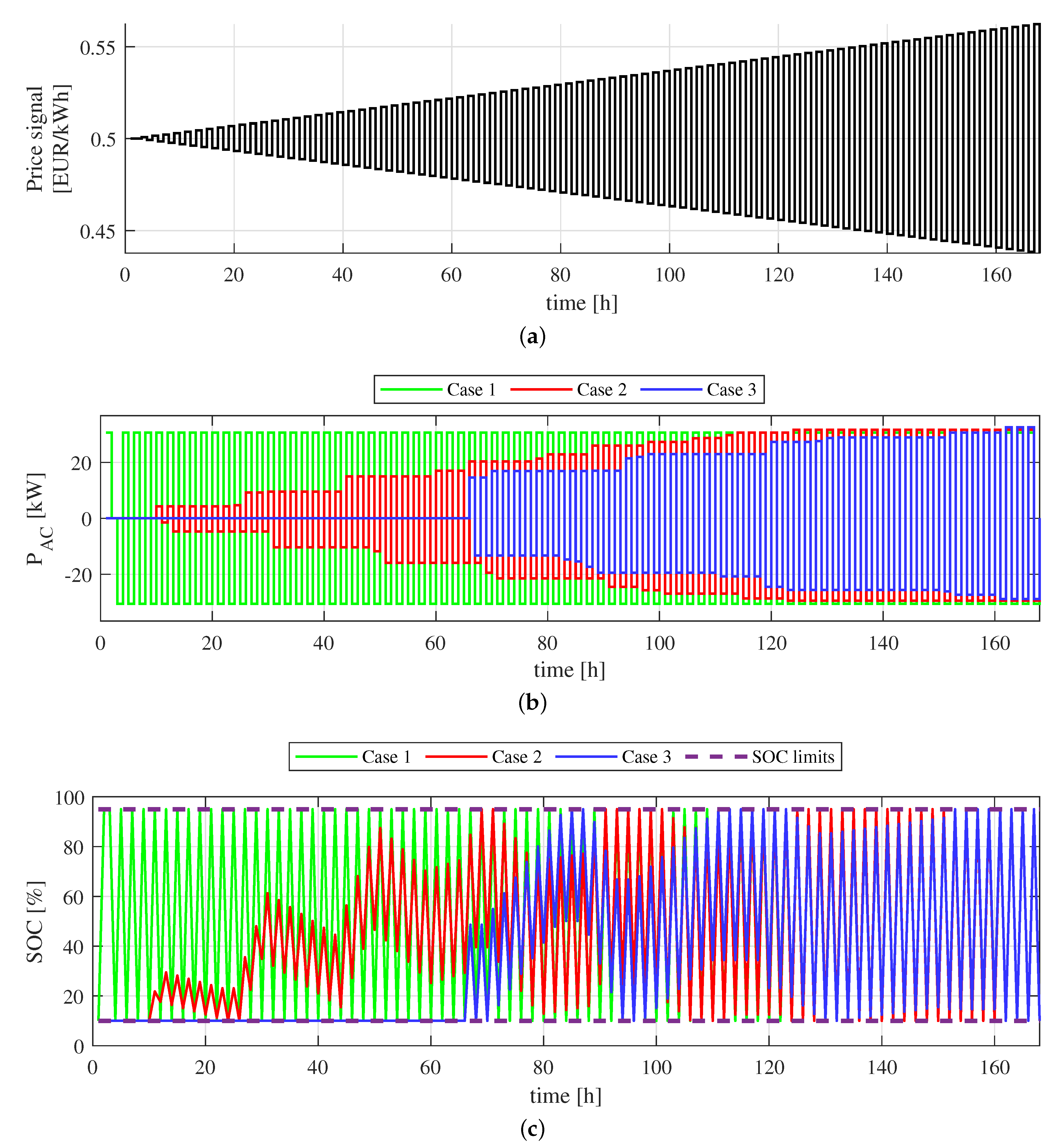
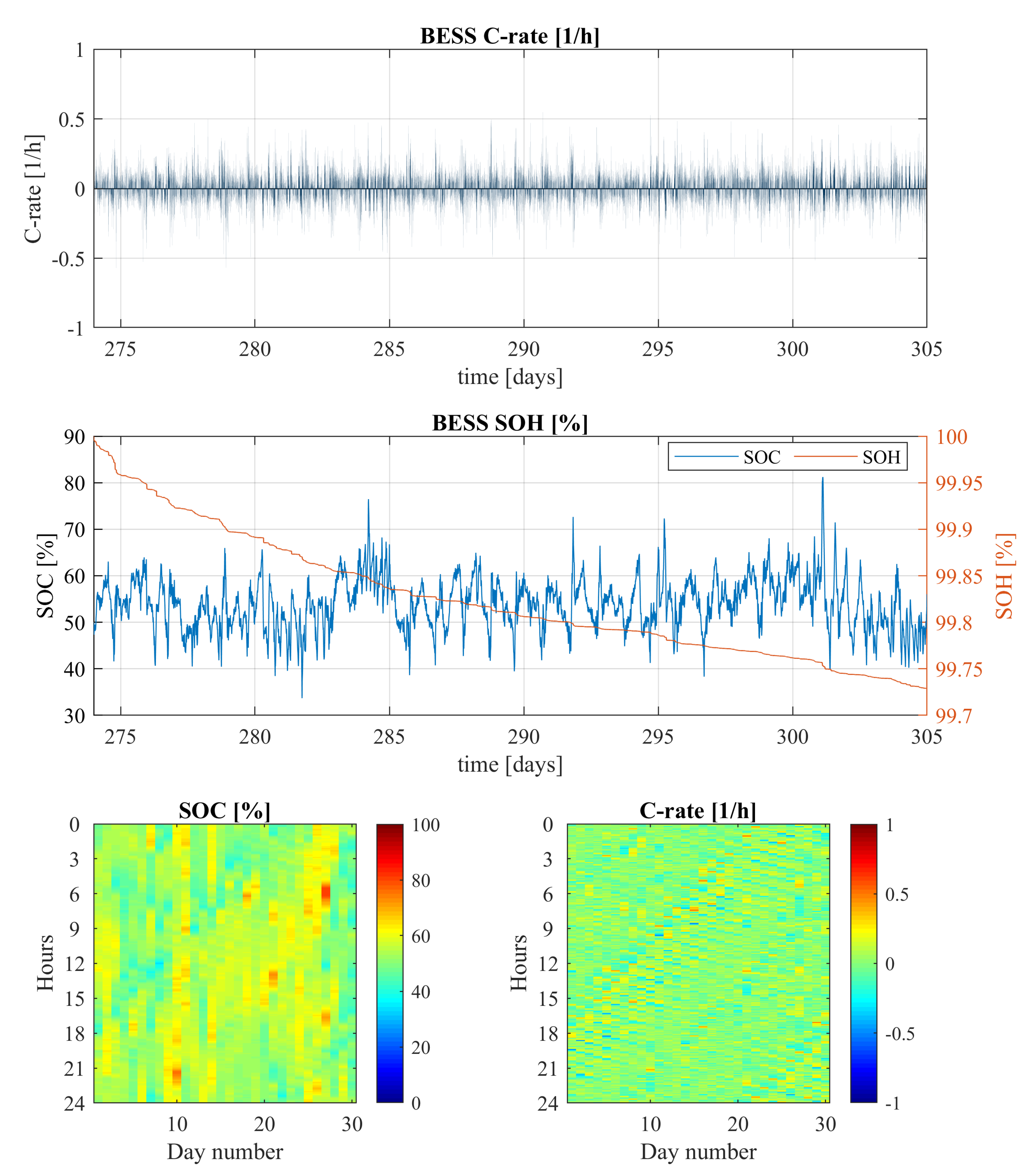
Figure A4.
SimSES modelling of a 30 day PCR operation. The battery model is set to the lithium-iron-phosphate (LFP) cathode chemistry, and ageing is limited to cycle ageing solely.
Figure A5.
Ageing for: (a) Test data; (b) the intraday market; and (c) the day-ahead market.
Appendix A.1. PWA Approximation
The power of MILP lies in its ability to model highly complex functions using piecewise affine (PWA) approximations. Therefore, the nonlinear parts in the model, the ageing and loss functions, are modelled by suitable PWAs. As shown in
Figure A6,
is a nearly-quadratic (but not exactly) function of
. Therefore, these nonlinearities must be approximated by a series of PWA functions to use the MILP approach. However, since it is a convex function, the formulation can be done without using integer variables, which reduces the computational burden substantially.
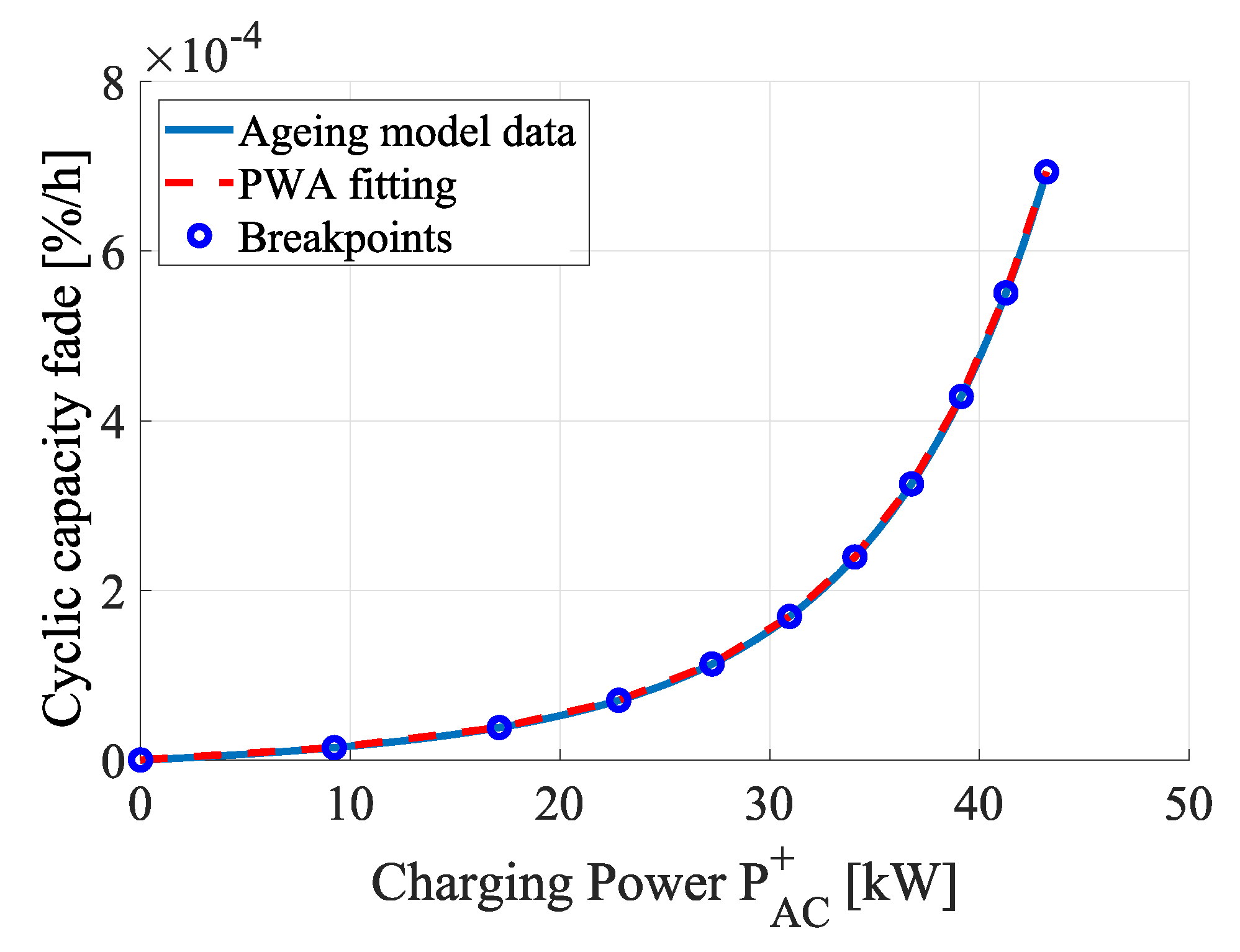
Figure A6.
Piecewise affine (PWA) curve fitting for the semi-empirical cycle ageing curve (charging).
Figure A6.
Piecewise affine (PWA) curve fitting for the semi-empirical cycle ageing curve (charging).
A sample PWA function is given in the form of Equation (
A1) and the actual function can be approximated by selecting the maximum value of the pieces, as in Equation (
A2) [
63].
This formulation can be converted into epigraph form, as in Equation (
A3) [
63]. In the epigraph form, a variable called
is defined as an upper boundary for all PWA functions. When an expression involving
is minimised,
will be minimised until it intercepts the maximum value amongst the PWA functions. Hence, it can accurately represent a convex PWA function.
After obtaining an appropriate form for approximation, the coefficients
and
, and the breakpoints
, in Equation (
A1), can be found by solving a nonlinear programming problem, defined by Equation (
A4) for a pre-defined
N number of pieces [
52]. Therefore, an open-source toolbox, developed by Alexander Szücs et al. [
64,
65,
66], is used to determine the unknown parameters. Solutions are given in
Table A4 and
Table A5.
Consequently, total ageing in the epigraph formulation is given by Equations (
A5) and (
A6).
In this formulation,
constitutes the upper bound for the PWA functions at each time step
k, similar to the role of
in the epigraph formulation given by Equation (
A3).
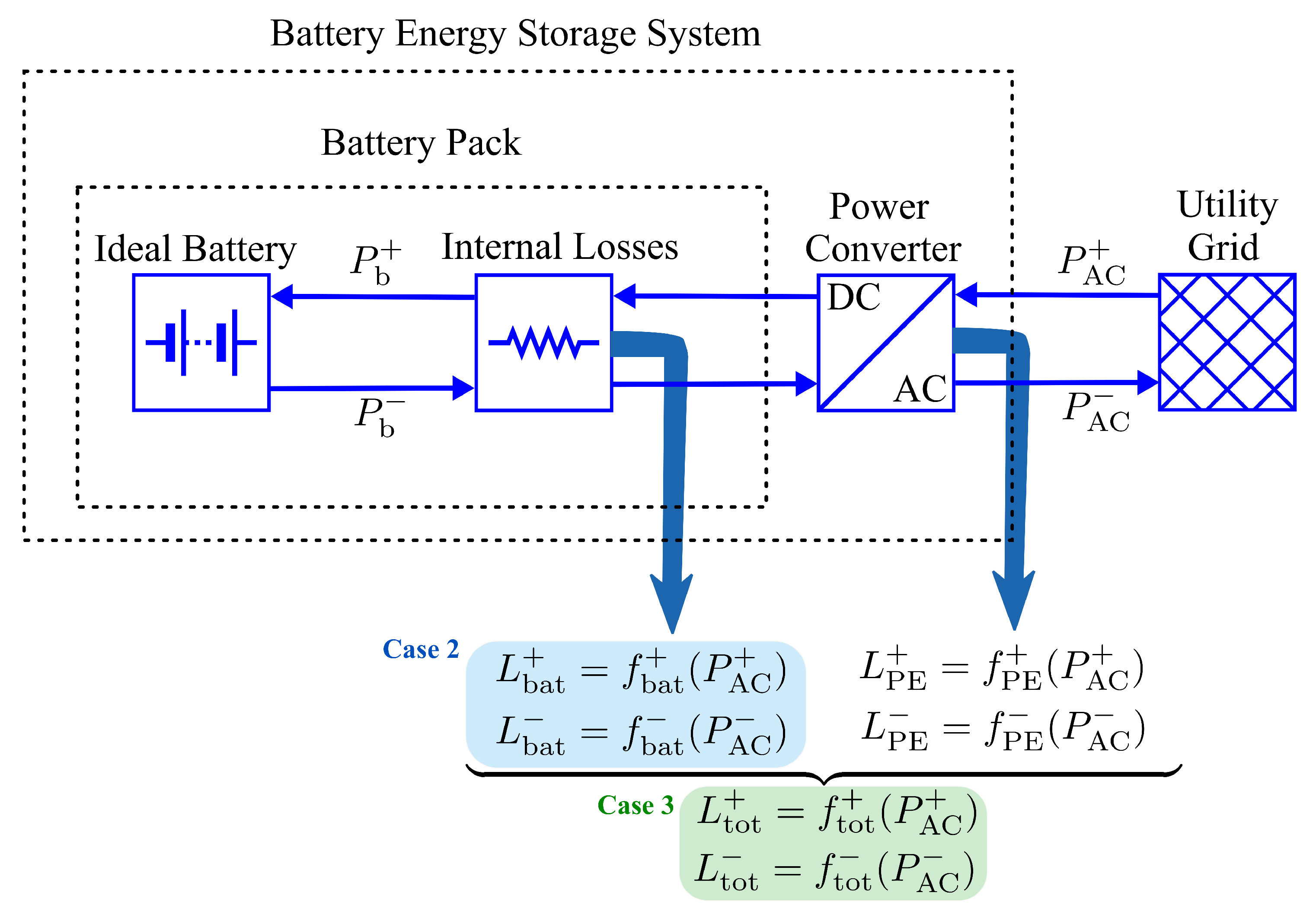
Appendix A.2. Battery Loss Modelling
In battery loss modelling, two loss elements are considered: Battery internal losses and power electronic losses [
14]. In this study, three cases are analysed: All losses are neglected (Case 1); only battery internal losses and ageing are considered (Case 2); and battery internal losses, battery ageing, and power-electronic losses are considered (Case 3). Therefore, as illustrated in
Figure A7, there exist different data-driven functions that map the input power
to the dissipation losses
(battery dissipation losses),
(power electronic losses) and
(total system losses). Loss mapping for Cases 2 and 3 is shown in
Figure A7, and
for Case 1. Therefore, according to the three different cases we study, there are four different functions
,
,
, and
(given in
Figure A8) to be approximated with the method given in the previous subsection.
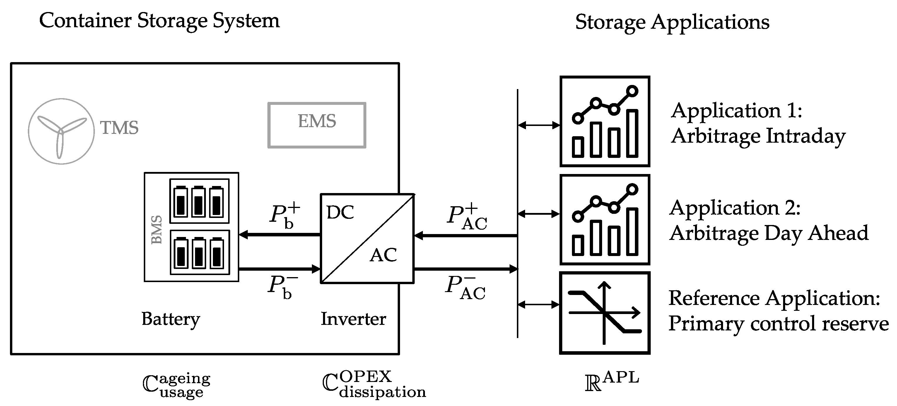
Figure A7.
System Diagram.
Figure A7.
System Diagram.
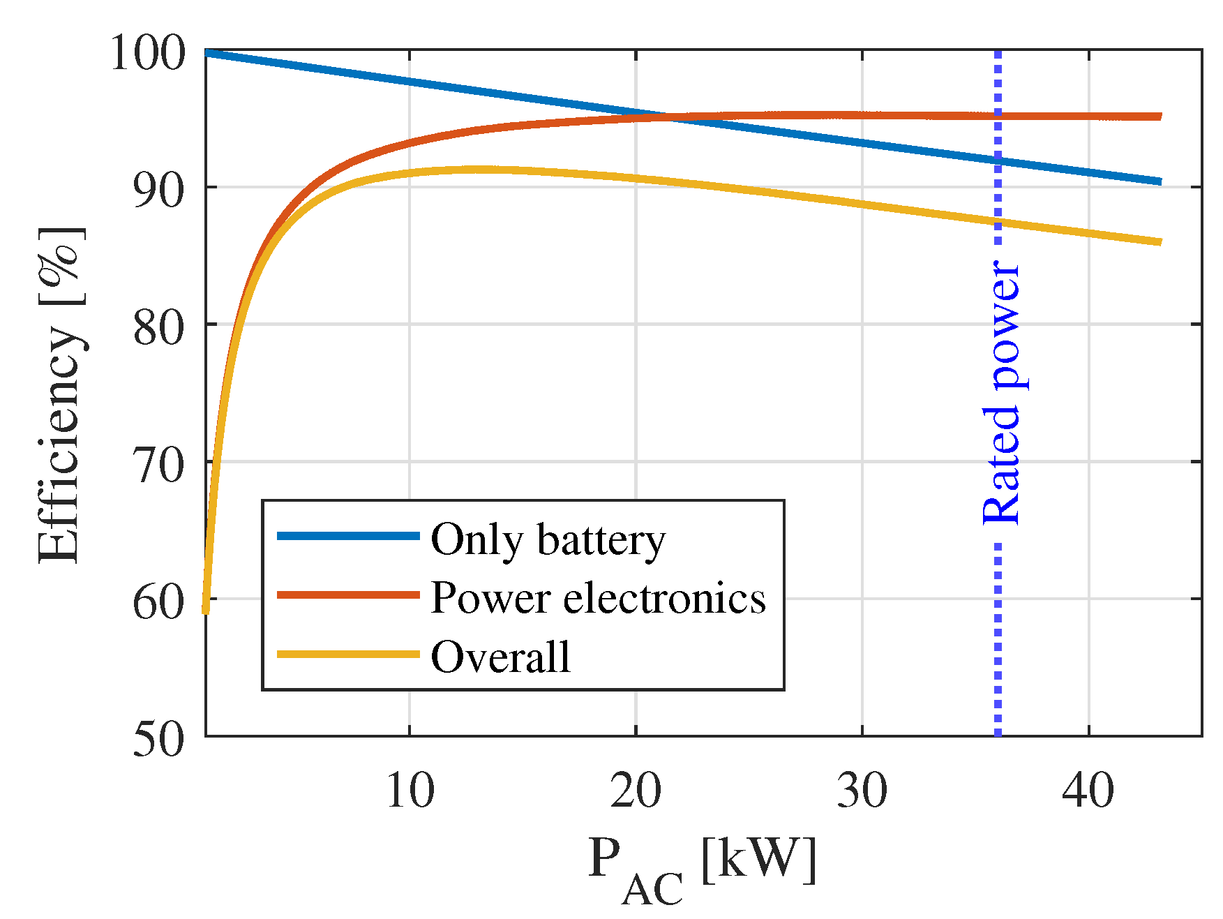
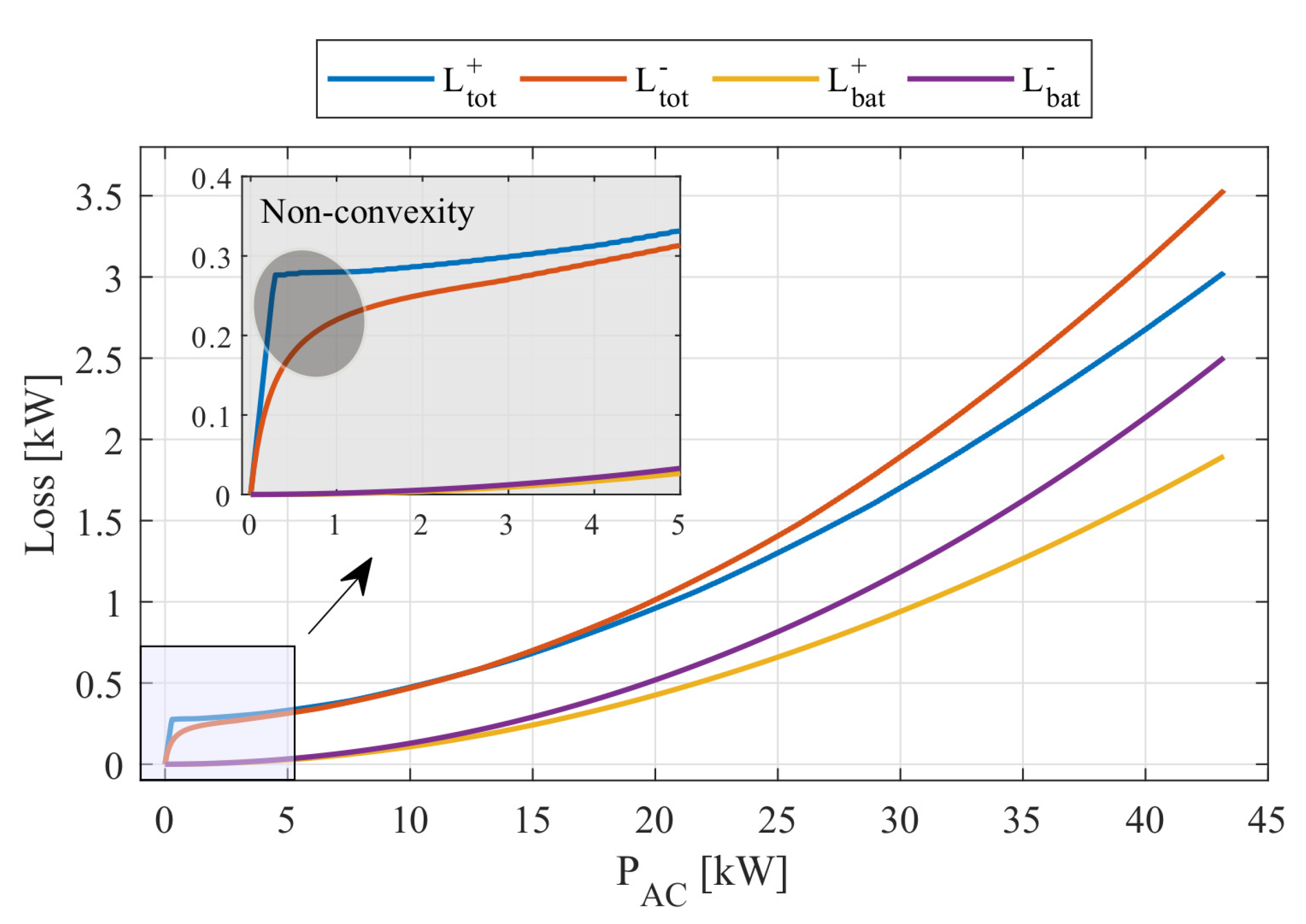
Figure A8.
Loss values for different AC side power levels.
Figure A8.
Loss values for different AC side power levels.
Compared to the PWA approximation of the ageing function, which is an increasing convex function, there are two complications for the modelling of the loss functions:
Some of the price values may be negative, which causes the loss function to be concave at that time step; therefore, the epigraph formulation given in Equation (
A3) cannot be used.
Although the battery loss functions
and
are convex, the combined loss functions
and
are non-convex. Hence, they can not be written as in Equation (
A3).
Due to the above problems, the representation in Equation (
A3) cannot be completely relied on for selecting the appropriate part of the PWA function. Therefore, we need to expand our formulation into the mixed-integer domain to include binary variables, which can be utilised to select the correct segment of the PWA function. However, despite having the state-of-the-art MILP solvers, excessive use of integer variables may lead to an insufficient memory problem and an increased computation time. Hence, we utilise a decomposition method that will reduce the number of redundant binary and real variables. The procedure followed is produced in
Figure A9 and
Figure A10.
The procedure given in
Figure A9 and
Figure A10 is basically a classifier that makes rough decisions to determine if a part of the system is convex, non-convex, or concave, which are collected, respectively, in the sets
,
, and
. The algorithm assumes that the PWA approximations are mostly convex, and that there are only several pieces that violate the convexity condition. The validity of this assumption can be verified by
Figure A8. Only a small portion of
causes non-convexity. Therefore, using binary variables to represent all segments is not necessary. For this reason, the function can be split into several regions that are convex themselves and fewer binary variables that can be utilised to select amongst these regions instead of all piece-wise functions. Inside each different region, the epigraph formulation can be leveraged to select the correct piece. On the other hand, as given in Equation (
7), the cost incurred by the efficiency losses is embedded in the first term, and it can be expanded into Equation (
A7) by using Equations (
10)–(
12):
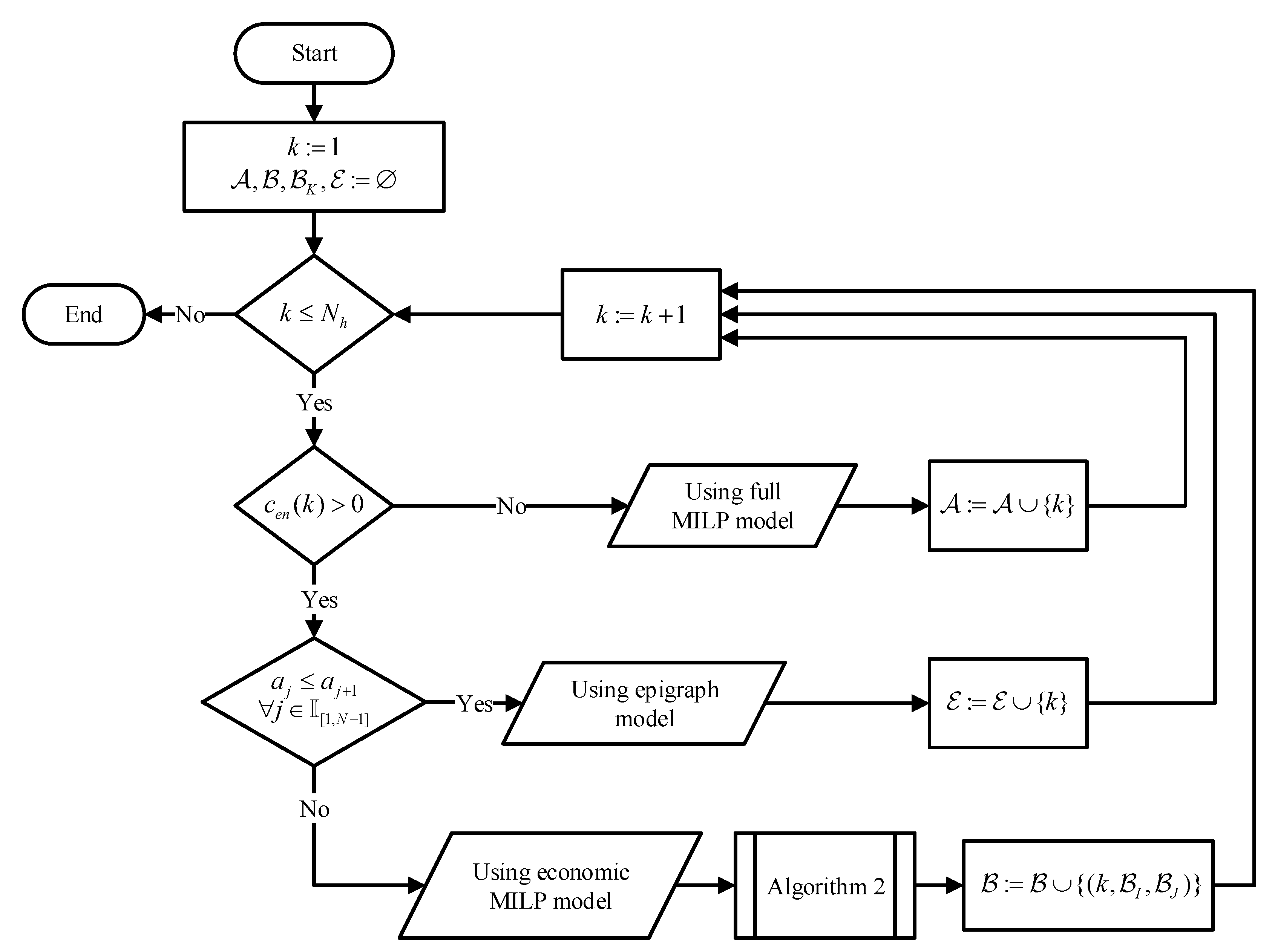
Figure A9.
Flowchart to determine approximation method for losses.
Figure A9.
Flowchart to determine approximation method for losses.
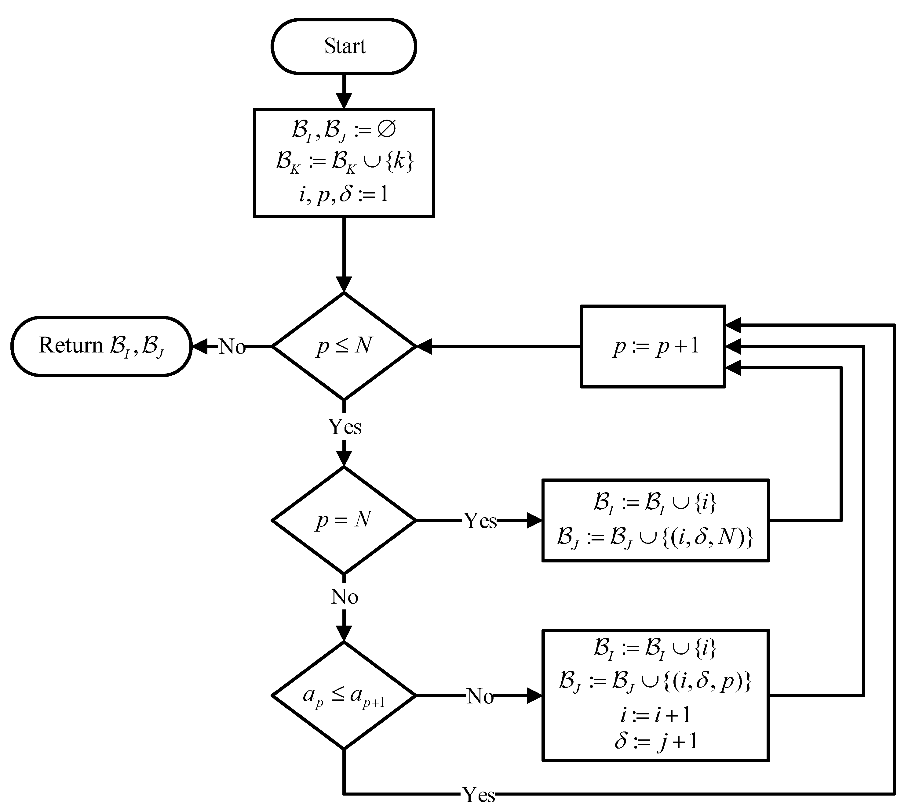
Figure A10.
Flowchart for Algorithm 2.
Figure A10.
Flowchart for Algorithm 2.
For the epigraph formulation to hold, the approximated variables, shown in Equation (
A7), must be minimised in the optimisation problem. However, if the multiplier
at time
k is negative, the loss values in the brackets are going to be maximised by the optimisation solver. In other words, having a negative price signal at time
k causes the curves shown in
Figure A8 to be reversed and become concave or mostly concave. Therefore, a full-scale MILP formulation with binary variables assigned for each piece in the PWA approximation must be used. In summary, when the price signal is negative, the loss function is multiplied by a negative number and converted into a mostly concave function. In this case, the algorithm executes the complete MILP modelling at that time step. If the price signal is not negative, but the PWA approximation violates the convexity requirement at some points (e.g., the slope is not monotonically increasing), then the algorithm collects all breakpoints and the time step in the set
. Lastly, if the PWA approximation is completely convex, then the procedure given in
Appendix A.1 (the previous section) is applied.
After the problem separation, the final equations to complete the system formulation are given. First, the
a,
b, and
r coefficients and breakpoints must be defined in the system, according to the studied case (where the numerical values are presented in
Table A4). Selected parameters for charge and discharge will be called
,
, and
, and
,
, and
, respectively. Then, by leveraging the algorithm given in
Figure A9 for both charge and discharge approximations, the sets
,
, and
, and
,
, and
are obtained, respectively. Then, we define two group of variables for the full MILP and economic MILP models. Binary variables are shown by
S, where continuous variables are given by
P, with indices full and eco for full MILP and economic MILP, respectively. finally, the variables related to charging and discharging are indicated by a plus and minus sign as superscript, respectively. Therefore, the newly defined variables are given by
,
,
,
,
,
, and
,
, in respective sets of appropriate dimensions. Thereafter, we define the following constraints. For all
k that the epigraph formulation can be used, the constraints are defined by Equations (
A8) and (
A9).
For all
k that the full MILP formulation must be used, the constraints are defined by Equations (
A10)–(
A15).
For all
k that the economic MILP formulation can be utilised, the constraints are defined by Equations (
A16)–(
A21).
Table A4.
PWA approximation parameters for power loss ( is omitted).
Table A4.
PWA approximation parameters for power loss ( is omitted).
| Efficiency |
|---|
| Charging | Discharging |
|---|
| Case 2 | Case 3 | Case 2 | Case 3 |
|---|
| a | b | r | a | b | r | a | b | r | a | b | r |
| () | [kW] | [kW] | () | [kW] | [kW] | () | [kW] | [kW] | () | [kW] | [kW] |
| 3.29 | 0 | 4.26 | 1000 | 0 | 0.29 | 4.71 | 0 | 4.68 | 467.65 | 0 | 0.44 |
| 14.99 | −0.0498 | 9.57 | 12.14 | 0.2655 | 5.33 | 19.31 | −0.0684 | 10.34 | 24.18 | 0.1955 | 7.74 |
| 26.26 | −0.1577 | 14.94 | 30.3 | 0.1688 | 10.97 | 33.98 | −0.2202 | 15.93 | 39.5 | 0.077 | 13.3 |
| 37.23 | −0.3216 | 20.39 | 46.17 | −0.0052 | 16.95 | 48.89 | −0.4576 | 21.46 | 58.97 | −0.1821 | 19.47 |
| 47.97 | −0.5406 | 25.97 | 61.36 | −0.2627 | 22.96 | 64.07 | −0.7835 | 26.94 | 78.7 | −0.5662 | 25.66 |
| 58.56 | −0.8155 | 31.68 | 76.69 | −0.6147 | 28.94 | 79.74 | −1.2054 | 32.41 | 101.55 | −1.1526 | 31.62 |
| 68.86 | −1.1419 | 37.39 | 91.77 | −1.0513 | 35.17 | 95.58 | −1.7188 | 37.84 | 118.59 | −1.6915 | 37.56 |
| 79.01 | −1.5213 | 43.2 | 104.71 | −1.5062 | 43.2 | 111.67 | −2.3276 | 43.2 | 135.27 | −2.3179 | 43.2 |
Table A5.
PWA approximation parameters for cycle ageing ( is omitted).
Table A5.
PWA approximation parameters for cycle ageing ( is omitted).
| Cycle Ageing |
|---|
| a () | b () | r |
| [ h/kW] | [] | [kW] |
| 1.44 | 0 | 9.24 |
| 2.97 | −0.142 | 17.11 |
| 5.62 | −0.594 | 22.8 |
| 9.58 | −1.5 | 27.25 |
| 15.1 | −3.01 | 30.94 |
| 22.5 | −5.28 | 34.06 |
| 31.8 | −8.47 | 36.76 |
| 43.4 | −12.7 | 39.13 |
| 57.3 | −18.1 | 41.26 |
| 73.7 | −24.9 | 43.2 |

 ,
, 


