Daily Operation Optimization of a Hybrid Energy System Considering a Short-Term Electricity Price Forecast Scheme

Abstract

The scenario where the renewable generation penetration is steadily on the rise in an increasingly atomized system, with much of the installed capacity “sitting” on a distribution level, is in clear contrast with the “old paradigm” of a natural oligopoly formed by vertical structures. Thereby, the fading of the classical producer–consumer division to a broader prosumer “concept” is fostered. This crucial transition will tackle environmental harms associated with conventional energy sources, especially in this age where a greater concern regarding sustainability and environmental protection exists. The “smoothness” of this transition from a reliable conventional generation mix to a more volatile and “parti-colored" one will be particularly challenging, given escalating electricity demands arising from transportation electrification and proliferation of demand-response mechanisms. In this foreseeable framework, proper Hybrid Energy Systems sizing, and operation strategies will be crucial to dictate the electric power system’s contribution to the “green” agenda. This paper presents an optimal power dispatch strategy for grid-connected/off-grid hybrid energy systems with storage capabilities. The Short-Term Price Forecast information as an important decision-making tool for market players will guide the cost side dispatch strategy, alongside with the storage availability. Different scenarios were examined to highlight the effectiveness of the proposed approach.

1. Introduction

Over the last decade we have witnessed a renewable energy burst. This flourishing, increasingly mature and less costly portfolio of renewable generation technologies, with a prominence of wind, hydro, solar, biomass, geothermal and ocean energy technologies [1,2], offers a variety of clean and environment-friendly energy sources. These are responsible for an ever-increasing supply share of electric loads (rising electrification rate), shifting from a centralized energy mix, i.e., an upstream grid based on circumscribed fossil fuels (prone to price increase with considerable economic spillovers) and nuclear energy, towards a rich renewable energies’ portfolio [3,4]. The scientific community, as well as policy makers, have set ambitious goals for the energy sector, particularly in Europe that, in addition to its commitment to the Paris Agreement, has targeted an almost emission-free generation in Europe by 2050 (Energy Roadmap 2050). According to recent data reports, 167 GW of new renewable power capacity was added, in 2017 alone, totaling now more than 2 TW of global renewable energy generation capacity, surpassing the already astounding figure of 138.5 GW added in 2016, which in itself was approximately equivalent to Canada’s total installed capacity [5,6]. With this regard, we must emphasize the levels of photovoltaics integration, either in self-consumption or mandatory grid injection schemes, with both residential and buildings appliances adding up to a third of the globally installed PV capacity [7]. Even though these technologies present some drawbacks, specifically their dependence upon weather conditions (stochastic nature), making them too unreliable to meet the whole energy demand, which in unconnected systems can lead to supply disruptions [8,9].

An hybrid energy system (HES) is typically formed by matching different forms of renewable/non-renewable energy sources with or without storage units in order to achieve a greater balance in the energy supply (mitigating its uncertain nature), a more distributed generation, as well as an increased system reliance [8,9], i.e., by better exploiting the local endogenous resources, taking advantage of the combined production from different technologies, e.g., solar photovoltaic, solar thermal, wind, hydro, biomass, hydrogen, fuel cells, micro-turbine generators, diesel generators among others. As a result of the wide range of existing technologies, innumerous HESs have been proposed, combining all sorts of generation technologies to deal with both generation and load uncertainty, in different topologies and operating strategies [2,3,4,10,11,12,13,14,15,16,17]. For instance an optimal scheduling approach for a thermal-wind-solar system with storage, considering the uncertainty in load forecast, and in wind and solar power output is proposed in [14], another example is the stand-alone wind-photovoltaic-hydrogen presented in [18]. In another instance, a maritime solution anticipating the increasingly high costs of fossil fuels and increasing restrictions on diesel usage and gas emissions from ships was proposed. Its operation is based on an optimal PV/battery/diesel scheme during the cold-ironing connection. A solar HES with diesel generators is contemplated (via Homer^®) in [19] to respond to the growing demand on isolated telecommunication infrastructures in Nigeria. This type of hybrid renewable energy systems integration is an effective electrification solution, in particular for rural electrification in least developed countries. Following this path, an off-grid hybrid PV-diesel-battery appliance (with an optimization based on PSO and ε-constraint method) serving a demand of 20 households in remote Saharan regions with 93% renewable fraction is proposed in [20]. A multi-objective optimization of the power dispatch of a large-scale integrated energy system (distributed district heating and cooling units and a power grid) via adaptive covariance and Lévy flights was assembled in [21]. Lastly, a rule-based method is implemented in [17] to a PV, wind, diesel and battery energy storage system via minimizing the operation cost by scheduling the distributed energy resources.

Besides, these systems can operate as “grid-connected” or “off-grid”, i.e., as stand-alone systems, constituting a suitable solution for rural and isolated areas (ranging from suitable HES for remote islands to particular alternatives for buildings) with demand and resource availability [1,2,4,11,16,22]. However, the optimized operation of these systems still poses some challenges. For all these reasons, HESs are presently a hot topic among researchers [4], covering topics ranging from feasibility analysis, optimum sizing, modeling, dispatch, control aspects and reliability issues [9,23].

Furthermore, one of the most important tasks regarding HESs is the generation and storage operation control, known as dispatch strategy. Load Following, Cycle Charging and Combined Dispatch are the most employed classical strategies. A common complementary strategy is the use of demand and/or renewable generation forecasts to outline the charging periods of the battery bank, usually known as Predictive Dispatch [24,25].

As a matter of fact, these HES together with demand-response mechanisms, constitute a great opportunity for industrial, commercial and public prosumers (active energy consumers), whose primary activity is not electricity generation, but who possess the necessary capital and land resources to collect the energy savings. Moreover, benefiting from the fall in the cost of renewable energy technologies and by actively participating as players in the “broader” horizontal electricity markets, can make them achieve noteworthy profits [26,27]. In this framework, this research proposes an optimal dispatch strategy for a simulated grid connected/stand-alone hybrid energy system, owned by an industrial prosumer with resources availability. Contemplating the common PV/Wind (onshore) generation in simultaneous operation mode [23], as well as a traditional energy storage unit (battery), complemented by the addition of a less common small hydro unit with pumping that, in parallel to the battery bank, will provide storage capability. This is a particular feature since few research works have explored HES with both multi-generation units and multi-storage units [22]. The operating strategy proposed in this paper, essentially, can be decomposed into two phases. In the first phase a short-term electricity price forecast (24 h-ahead) is carried out, using a feed forward neural network (FFNN). In a second phase, a real-time dispatch is performed subject to several constraints, incorporating the short-term price forecast and the current state-of-charge of the storage units, to allow the best compromise between cost and reliability of the various generation and storage technologies, i.e., satisfying the electricity demand while minimizing the operation costs. The main contributions of this work can be defined as:

• A new hybrid energy system architecture is proposed, combining a wide-range of technologies, including a Pumped Storage Hydro unit as a complementary storage technology;
• A novel dispatch strategy (algorithm) based on a 24 h electricity price forecast coupled with the state-of-charge information from the storage technologies is presented;
• In addition to the main grid-connected mode, the novel dispatch strategy contemplates modifications to the algorithm (cost formulas) for the off-grid operation (standalone mode), with the addition of traditional diesel generators.

This paper is organized as follows: Section 2 describes the proposed hybrid topology and its operating principles (operation assumptions) and formulates the PV/wind/PSH/diesel/battery optimal dispatch strategy. The case study is presented in Section 3, explaining the prosumer profile replicated in this paper and illustrating the used input variables. Section 4 briefly describes the current electricity market structure (where our industrial prosumer is inserted), the importance of Short-Term Price Forecasting as a decision-making tool and finally the approach followed in this paper, including its data preprocessing stage. Then, in Section 4 the modeling of the HES is presented, including all the specifications employed. In Section 5, the case study is simulated in different scenarios and its results are highlighted, before closing this work in Section 6 with the main conclusions.

2. System Architecture and Operation

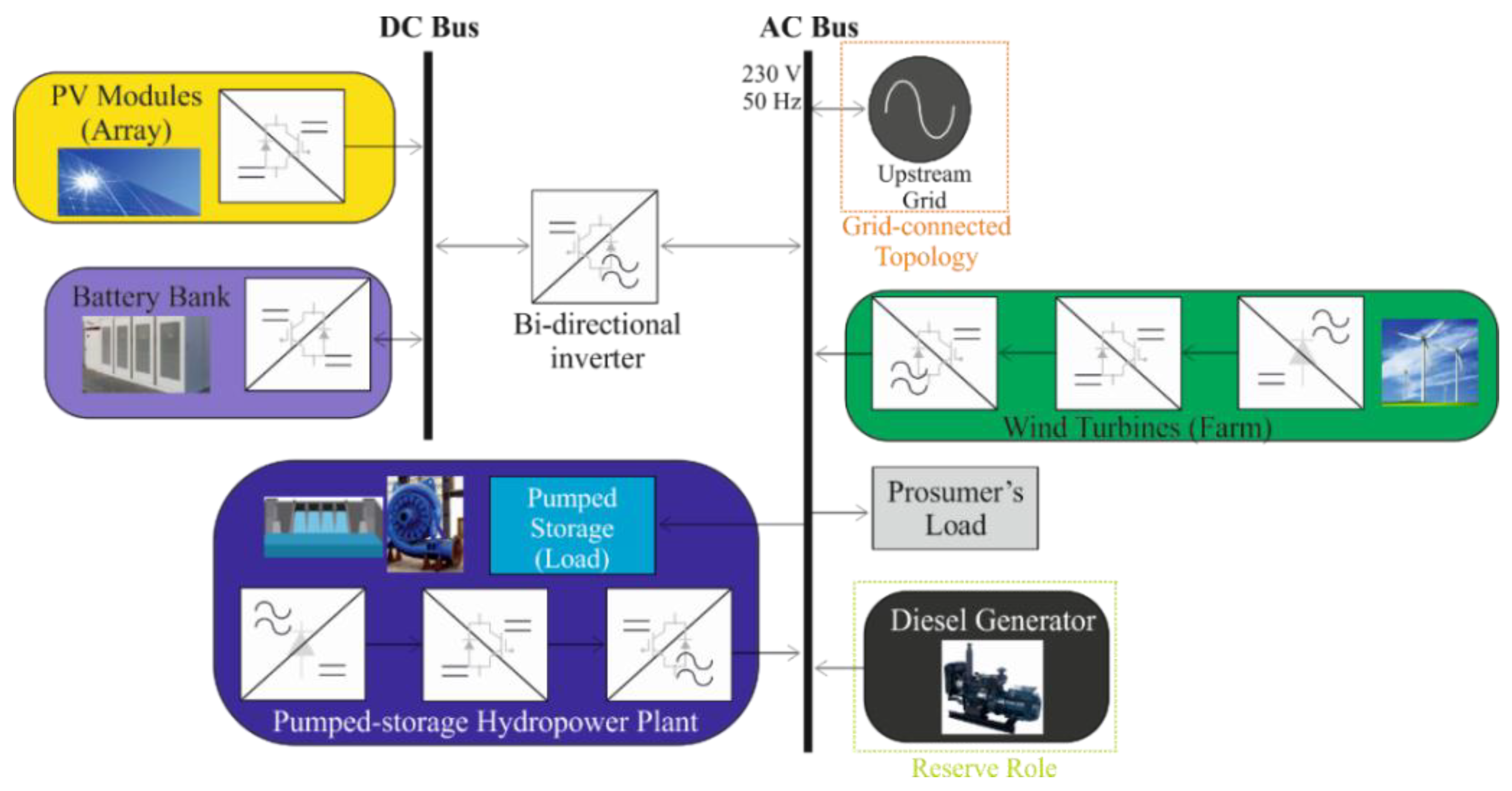
The underlying hybrid architecture, interconnected with the grid, combining the generation technologies (PV-wind-PSH-diesel) and the storage unit mentioned above, is illustrated in Figure 1. An advantage of this architecture is the plug-and-play operation, where wind, hydropower and diesel generation units are coupled directly to the AC Bus. The storage unit (battery bank) and the PV generation are coupled to a DC bus, through proper DC/DC converters, which is then sequentially coupled to the AC bus through a bidirectional DC/AC, thus allowing a two-way (flow between the two busbars) power flow. The diesel generator will play a reserve role, i.e., its primary state is off, only on shut down situations will be turned one, otherwise the grid exchanges will provide existing shortages.

The proposed HES, shown in Figure 1, was designed to fully satisfy an actual load profile for a simulated prosumer profile. The overall operation strategy pseudocode is formulated above (Algorithm 1), it starts with a data gathering and features extraction stage (i), where the different time-series are analyzed and processed. Subsequently, the short-term price forecasting (ii) is carried out for a one-day ahead horizon, using a FFNN as a forecasting engine. These procedures are further explained in Section 4.

Algorithm 1: Proposed operation strategy

i. init: Data gathering and Features Extraction ii. price forecasting$\left\{{\widehat{p}}_1,\text{}{\widehat{p}}_2,\mathrm{\dots },{\widehat{p}}_{24}\right\}$ iii. for$k=1:K_{\mathrm{N}}$ iv. $\mathsf{\epsilon }\left(k\right)=P_{\mathrm{D}}\left(k\right)-\left(P_{\mathrm{solar}}\left(k\right)+P_{\mathrm{wind}}\left(k\right)\right)$ v. $\min \left\{\begin{array}{c}{C}_{\mathrm{solar}}{P}_{\mathrm{solar}}\left(k\right)+C_{\mathrm{wind}}{P}_{\mathrm{wind}}\left(k\right)+C_{\mathrm{grid}}\left(\mathsf{\epsilon }\left(k\right)\right)P_{\mathrm{grid}}\left(k\right)+\\ +{\displaystyle {\sum }_{j=1}^2{C}_j\left(SO{C}_j\left(k\right),\Delta SO{C}_j,\widehat{p}\left(k\right)\right)P{g}_j}\end{array}\right\}$ System constraints: vi. $P_{\mathrm{solar}}\left(k\right)+P_{\mathrm{wind}}\left(k\right)+P_{\mathrm{grid}}\left(k\right)+{\displaystyle {\sum }_{j=1}^{2}P{g}_j\left(k\right)=P_{\mathrm{D}}\left(k\right)}$ vii.  if$\mathsf{\epsilon }\left(k\right)>0$ then $P{g}_1\left(k\right)>0$ $P{g}_2\left(k\right)>0.1P_{\mathrm{hydro}\mathrm{rated}}$ $P_{\mathrm{grid}}\left(k\right)>0$ viii.  else $P{g}_1\left(k\right)\le 0$ $P{g}_2\left(k\right)\le -0.1P_{\mathrm{hydro}\mathrm{rated}}$ $P_{\mathrm{grid}}\left(k\right)\le 0$ ix.  end if x. $\{\begin{array}{c}P{g}_{j,\min }\left(k\right)\le P{g}_j\left(k\right)\le P{g}_{j,\max }\left(k\right)\\ P_{\mathrm{grid}}\left(k\right)\le P_{\mathrm{grid},\max }\end{array}$ xi. end for xii. end

Following the forecasting stage (ii), for each discrete-time step k, up to a total of K_N steps (simulation time horizon), it is determined how much the non-dispatchable PV and wind generations can supply the existing load P_D(k) given by $\mathsf{\epsilon }(k)$ (iv). This will result in situations where $\mathsf{\epsilon }(k)>0$, i.e., energy deficit, which involves the discharge of the storage technologies or the purchase of energy from the grid. On other hand, when $\mathsf{\epsilon }(k)\le 0$, i.e., energy surplus, requiring that the energy surplus is either stored in the storage technologies or sold to the grid.

Thereafter, the economic dispatch is carried out, i.e., allocating the available generation to supply the HES load, while minimizing the operation costs (v) and fulfilling the demand–supply balance (vi) and unit capacity limits constraints (x).

In (v) the economic dispatch (ED) stage is executed by linear programming, determining the output power of the different units that form the proposed HES, to fulfill the existing energy deviation $\mathsf{\epsilon }(k)$ in the most cost-effective manner. C_solar, C_wind, C_j and C_grd are the costs associated with the respective generation technologies and the grid electricity cost (energy price), respectively. In particular, C_j translates the storage unit and pumped-storage hydro plant (PSH) cost as defined in Equation (2) and are computed as a function of the state of charge, SOC_j, and an estimate of how much the SOC of the storage technologies varies, ΔSOC_j, as well as the forecasted prices, $\widehat{p}\left(k\right)$, where the index j selects the battery bank for j = 1 and PSH as a source/sink for j = 2. In the case of the PSH, SOC₂ is defined as the ratio between the current volume of stored water and the reservoir maximum capacity. Equation (2) was defined as a piecewise function where each sub-function has its own SOC_j, working range and signal of $\mathsf{\epsilon }(k)$. The considered SOC working range for both storage technologies were [0.15,1], implying that the domain of ΔSOC_j is [−0.85,0.85].

The marginal costs of the non-dispatchable generation are considered null. Regarding the grid cost, the same is computed as a function of the state of charge, SOC_j, and the electricity price forecast (predicted value $\widehat{p}$, predicted daily average and maximum predicted value) and is given by Equation (1). This cost was also defined as a piecewise function where each sub-function is defined over an interval formed by the signal of $\mathsf{\epsilon }(k)$ and $\widehat{p}\left(k\right)$. The inclusion of the electricity price forecast information on the formulation allows to gauge the future trend of electric energy prices, which is of high interest for a player with this type of generation mix. Since it allows to dispatch the stored energy when high electricity prices are expected and, on the opposite, to take advantage of off-peak periods for storing energy when lower electricity prices are expected.

For instance, in the presence of energy deficits, $\mathsf{\epsilon }(k)>0$, the $SO{C}_j(k)$ is inversely proportional to the attributed grid cost, furthermore a normalized price information $\frac{1}{24}{\displaystyle \sum _{j=1}^{24}{\widehat{p}}_j}\text{}/\max \left(\left\{{\widehat{p}}_1\mathrm{\dots }{\widehat{p}}_{24}\right\}\right)$ regarding the considered day will translate how the average compares with the maximum forecasted value, finally the predicted $\widehat{p}\left(k\right)$ price for the current hour is compared with its daily average, decreasing the grid cost if $\widehat{p}\left(k\right)<\text{}\frac{1}{24}{\displaystyle \sum _{n=1}^{24}{\widehat{p}}_n}$ and otherwise increasing it, in turn for the energy surplus situation, $\mathsf{\epsilon }(k)\le 0$, the $SO{C}_j(k)$ is now directly proportional to the attributed grid cost and instead of adding the factor regarding the difference between the current dispatch price and its daily average, the same is now subtracted.

From point (vi) forward, we focus the attention on the set of operational and system constraints to which the ED is subject. The first system operation constraint is the demand–supply balance equation (vi), translating the need for the non-dispatchable generation, $P_{\mathrm{solar}}\left(k\right)$ and $P_{\mathrm{wind}}\left(k\right)$, coupled with the sum of the output power from the PSH and battery bank units, $P{g}_j\left(k\right)$, as well as the power flow with the upstream grid, $P_{\mathrm{grid}}\left(k\right)$, to match at all times the HES load, $P_{\mathrm{D}}\left(k\right)$. In addition, it was established that for energy deficit occurrences, the output power $P{g}_j\left(k\right)$ and $P_{\mathrm{grid}}\left(k\right)$ have by convention a positive signal (vii), i.e., power is being injected into the buses (HES), contrarily, when $P_{\mathrm{grid}}\left(k\right)<0$ and $P{g}_j\left(k\right)<0$ power is now being injected into the grid and being consumed for pumping up the water (upstream reservoir) and/or to charge the storage bank (viii). Besides, an additional constraint concerning the operating range of the PSH unit is defined, imposing 10% of the rated power of the turbine, as minimum operating point both for turbine and pump modes (vii-b and viii-b). The last constraints (x) ensure that the power generation limits, firstly for battery bank, translates the lower and upper charge and discharge power, and secondly the generation/consumption bounds for the PSH unit, which are a function of the current $SO{C}_2$ and its generator rated power, $P_{\mathrm{hydro}\mathrm{rated}}$.

$$C_{\mathrm{grid}}\left(\widehat{p}\left(k\right),SO{C}_j(k)\right)=\{\begin{array}{c}\min \left(\left\{1-SO{C}_1(k)1-SO{C}_2(k)\right\}\frac{\frac{1}{24}{\displaystyle \sum _{j=1}^{24}{\widehat{p}}_j}}{\max \left(\left\{{\widehat{p}}_1\mathrm{\dots }{\widehat{p}}_{24}\right\}\right)}\right)+\frac{\widehat{p}\left(k\right)-\frac{1}{24}{\displaystyle \sum _{j=1}^{24}{\widehat{p}}_j}}{\max \left(\left\{{\widehat{p}}_1\mathrm{\dots }{\widehat{p}}_{24}\right\}\right)},\mathrm{if}\mathsf{\epsilon }(k)>0\wedge \widehat{p}\left(k\right)>0\\ \begin{array}{l}\min \left(\left\{SO{C}_1(k)SO{C}_2(k)\right\}\frac{\frac{1}{24}{\displaystyle \sum _{j=1}^{24}{\widehat{p}}_j}}{\max \left(\left\{{\widehat{p}}_1\mathrm{\dots }{\widehat{p}}_{24}\right\}\right)}\right)-\frac{\widehat{p}\left(k\right)-\frac{1}{24}{\displaystyle \sum _{j=1}^{24}{\widehat{p}}_j}}{\max \left(\left\{{\widehat{p}}_1\mathrm{\dots }{\widehat{p}}_{24}\right\}\right)},\mathrm{if}\mathsf{\epsilon }(k)\le 0\wedge \widehat{p}\left(k\right)>0\\ 0,\widehat{p}\left(k\right)\le 0\end{array}\end{array}$$

(1)

$$C_j\left(SO{C}_j(k),\Delta SO{C}_j(k),\widehat{p}\left(k\right)\right)=\{\begin{array}{c}2,\mathrm{if}\left(SO{C}_j(k)\le 0.15\wedge \mathsf{\epsilon }(k)>0\right)\vee \left(SO{C}_j(k)=1\wedge \mathsf{\epsilon }(k)\le 0\right)\\ \frac{\left(1-SO{C}_j(k)+\Delta SO{C}_j(k)\right)\left(\frac{1}{24}{\displaystyle \sum _{j=1}^{24}{\widehat{p}}_j}\right)}{\max \left(\left\{{\widehat{p}}_1\mathrm{\dots }{\widehat{p}}_{24}\right\}\right)},\mathrm{if}0.15\le SO{C}_j(k)\le 1\wedge \mathsf{\epsilon }(k)>0\\ \frac{SO{C}_j(k)\left(\frac{1}{24}{\displaystyle \sum _{j=1}^{24}{\widehat{p}}_j}\right)}{\max \left(\left\{{\widehat{p}}_1\mathrm{\dots }{\widehat{p}}_{24}\right\}\right)},\mathrm{if}SO{C}_j(k)<1\wedge \mathsf{\epsilon }(k)\le 0\end{array}$$

(2)

Lastly, several tweaks were also considered: for small discharge depths and state of charges close to 1 the cost of both technologies is similar; with state of charges close to 1 and as the discharge depth increases, the cost of using the battery bank is higher. This is especially important, since the battery bank is a more sensible storage technology, i.e., its preferable to avoid full discharges cycles, even if it requires charging cycles more frequently.

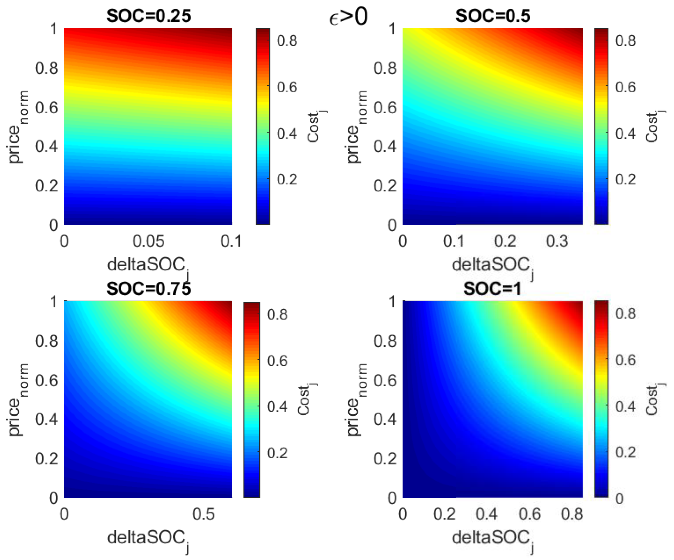
To better highlight the codomain of this cost function, Figure 2 is introduced, where four different initial SOCs are considered for an energy deficit situation (where a discharge of the storage technologies is expected). The chosen SOCs, were the upper limit, i.e., SOC = 1, followed by two intermediate levels (equally spaced), i.e., SOC = 0.5 and SOC = 0.75 and a near border limit of SOC = 0.85.

Figure 2 clearly shows that the cost is inversely proportional to the current SOC and varies in a way that favors the use of PSH and storage bank technologies when not only its SOCs are higher but also when the required DOD is smaller. Although the function ranges between [−1,1.85], for energy deficit situations its respective cost is always positive, since discharge cycles have negative repercussions on these technologies’ lifespan.

3. Case Study

The proposed daily operation optimization strategy for a HES (dispatch strategy) is tested under the assumption that a prosumer, such as a resourceful industrial/commercial corporation, has invested in an increasingly mature energy generation portfolio, firstly with the intent of suppressing/lessening their electric loads consumption burden, but also to take advantage of the decreasing storage cost, in other words to “act” as market player on both sides. Moreover, by taking advantage of the exchanges with the upstream grid, in foreseeable profitable periods, thus he accelerates not only the payback period (shortened), but also the medium-long term profitability. For example, the operation of a storage system owned by a large consumer that purchases electricity from the Ontario’s wholesale market, where the price forecasts are also applied to an optimization platform for operation scheduling of a battery energy storage system, within a grid-connected micro-grid in Ontario, is studied in [28].

For simulation purposes, it was necessary to use a nationwide database, which included not only all the parameters required to model the different HES sources, but also the vital information (explanatory/exogenous variables) for the successful implementation of a 24-h electricity prices forecasting in a real market context. To serve this purpose, the open power system data [29] was used. This online platform compiles national/system level data from several sources, not only containing common time-series data (load, prices and renewable generation and its respective forecasts, etc.), but also the important weather data (solar irradiation, temperature and windspeed). Thus, to include all the necessary simulation variables (used both in price prediction and in HES modeling), only a handful of countries provide all the necessary data on an hourly basis. In this sense, the data regarding the Czech Republic (CZ) system for the period from 1 January 2015 until 31 December 2016 was used. Furthermore, the annual average diesel prices for Czech Republic were also used to representatively model the diesel generator operation cost [30]. Nevertheless, some processing of these raw data is still necessary, starting with the necessary electric load adjustment, since the average CZ system load value is about 7343 MW, then a reducing scale factor is applied to bring the load to an average value around 100 kW (prosumer level). Secondly, since the wind speed is the result of average anemometers measurements across the country, its average value is around 3.93 m/s, which following the Wind Energy Resource Atlas of the United States for a height of 10 m placing it in the lowest class of wind power potential (class 1) and well below the majority of the wind turbines cut-in speed, when viable wind farming sites usually present values higher than 6 m/s. So, therefore, a scaling factor of 3 is applied to the existing wind profile to simulate more favorable conditions, as is customary in wind farm sites. In the same manner, a minor adjustment is applied to the irradiance levels, in order to better replicate more consistently the existing conditions in photovoltaic parks.

The existence of rebated fuel for off-road usage is a common practice in the vast majority of countries and is regulated in the European Union by the directive 92/81/EEC, which states in its Article 8 (2) that reduced rates or exemptions can be applied, namely for electricity production purposes. This type of fuel is often referred as colored or dyed fuel, and benefits from reduced taxes, for instance in the UK a VAT rate of 5% is considered for “red diesel” in contrast with the normal 20% VAT [31], and in Portugal fuels used to generate electricity are untaxed [32]. Consequently, for simulation purposes a 10% discount was considered when dealing with the end-user diesel prices, since industrial users benefit from a special regime.

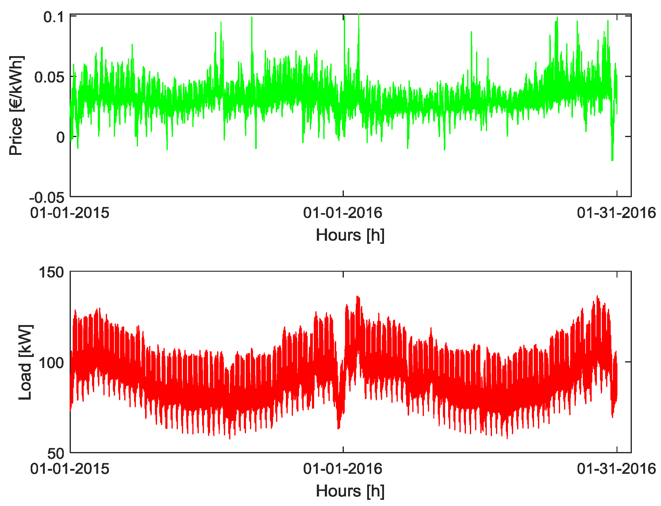
The electricity prices and the adjusted prosumer load profile are shown in Figure 3, in turn Figure 4 illustrates the employed meteorological data, whereas

Table 1. Descriptive statistics of the different datasets.

	Mean	Median	St. Dev	Minimum	Maximum	Skewness	Kurtosis
Prices [€/kWh]	3.17 × 10−2	3.07 × 10−2	1.28 × 10−2	−2.00 × 10−2	0.10	0.43	4.57
Load [€/kWh]	97.9	97.8	16.0	59.0	140.2	0.13	2.30
Wind Speed [m/s]	11.8	10.7	5.38	0.44	39.8	1.18	4.81
Irradiance [W/m2]	127.2	0.54	242.5	0	1193.3	2.17	6.94
Temperature [°C]	9.07	7.96	9.00	−12.0	36.2	0.37	2.41

provides the time-series descriptive statistics after the adjustments mentioned before, i.e., mean, median, standard deviation, upper and lower limits, as well as the shape related statistics, kurtosis and skewness for the hourly time-series. We can see a mean and median price around 3 cents per kWh, with a considerable standard deviation, in the order of 40% of the mean value (thus translating the difficulty for the forecasting task), a minimum negative value of 2 cents per kWh was recorded and the shape metrics reveal an approximately symmetric and leptokurtic distribution. The load was modeled with an average/median value of around 100 kW and presents also an approximately symmetric distribution, however kurtosis reveals a more compact distribution, i.e., platykurtic distribution.

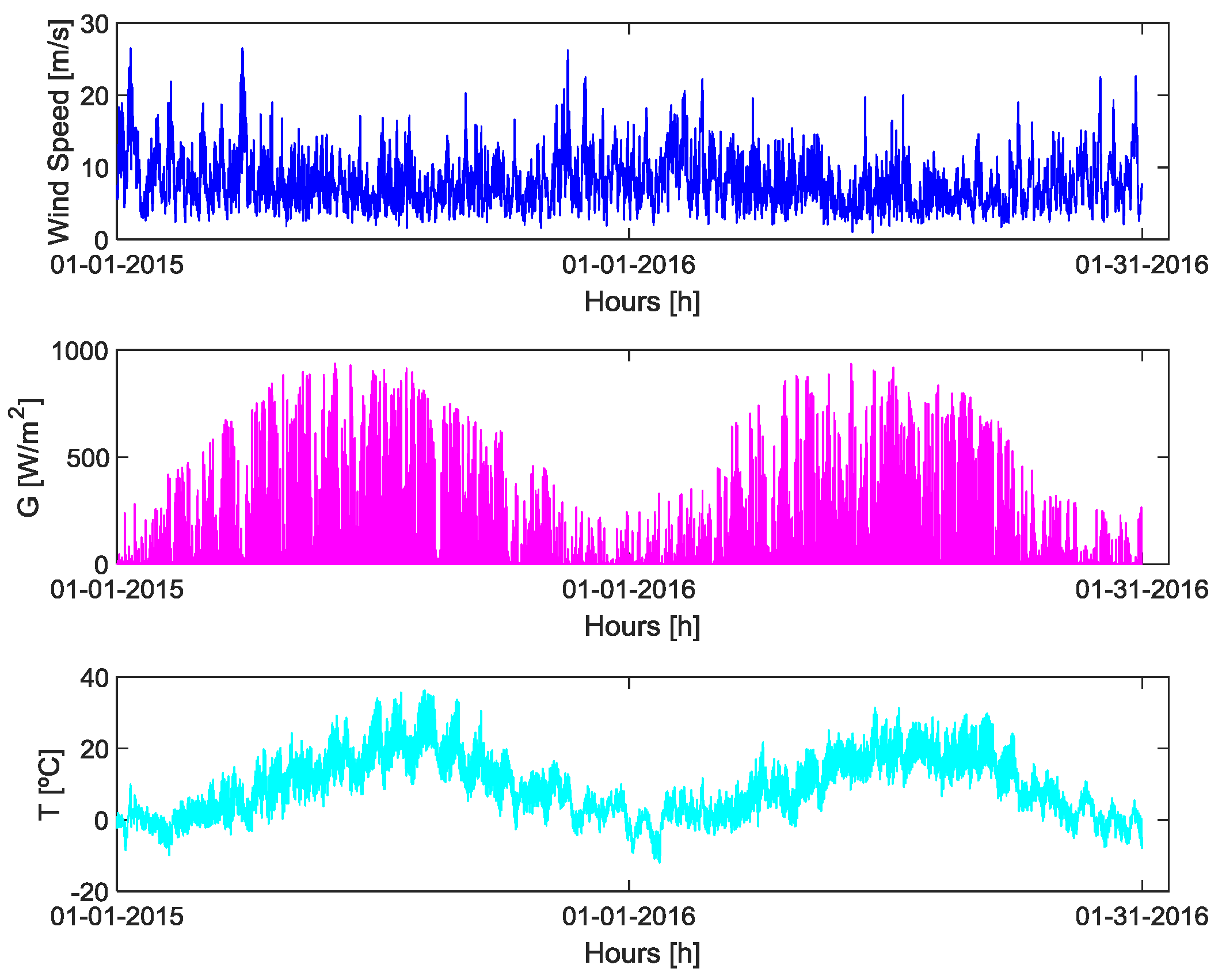
With respect to the wind speed profile, we can see that it presents a considerable standard deviation (in the order of 46% of the average value) with an adjusted average speed close to 11 m/s and the shape metrics reveals a leptokurtic and highly positively skewed distribution. The irradiance time-series further accentuates these shape characteristics. Furthermore, an interesting situation, where the standard deviation is higher than the mean and the median, has a considerably distance from the mean value of 127.2 W/m, revealing a very widely distributed data set. Meanwhile, temperature statistics reveal a time-series with relatively low mean temperatures and an approximately symmetrical distribution. Finally, we can also perceive that during the summer season, conditions are substantially more favorable for non-dispatchable generation.

For this permanent load levels, an energy portfolio totaling approximately 275 kW of non-dispatchable renewable sources (wind + solar) is considered, however, due to the unstable nature of these production sources, a traditional battery bank with an energy availability of around 130 kWh is added to the mix, accompanied by a small hydro unit which is one of the highlights of this paper, since it provides a second storage capacity and a nominal power around 150 kW. To conclude, the availability of diesel generators is also considered (~60 kW), to evaluate whether or not constitutes a viable alternative to the upstream grid exchanges, thereby as a preferred reserve source.

4. Short-Term Price Forecasting

The restructuring of the electric power systems saw deregulated wholesale energy markets emerge as effective structures to foster competition and override traditional vertically integrated utilities, enabling the participation of several entities such as generating and investment companies, distribution (retailers) companies, among others. Therefore, as widely traded commodity with special features (uninterruptable supply security and very limited storage capacity) electric energy (clearing) prices are set by intersecting the supply/demand curves [33,34,35]. However, a set of added taxes and levies must be accounted to determine the end user retail price, for instance in the first semester of 2018 they averaged approximately 30% of the household consumers retail electricity prices in the Euro Area. Besides, a distinction between household and non-household retail electricity prices needs to be considered, again for the 1 semester 2018 the Euro Area non-household prices were approximately 52% inferior [36].

In this framework, the existence of accurate price forecasts is an extremely important decision-making tool, mainly the day-ahead forecast, since it enables producers to hedge against risks and ultimately maximize their profits, while bulking consumers to optimize their load schedules. For the last few years, these wholesale markets have been dealing with increased volatility, thus making the forecasting task harder, much influenced by the snowballing levels of renewables and its particular close-to-zero marginal costs [33,37]. Hence, by following the Predictive Dispatch concept it is possible to model the operating costs of the implemented HES based on the information of these forecasting engines, in order to promote cost rationalization and its integrity (lifespan).

Plentiful methods have been developed for electricity price forecasting such as: statistical methods, computational intelligence methods and, nowadays with a greater propensity, hybrid methods [38,39,40,41]. These last further explore the best features of each individual method. Artificial intelligence techniques are among the favorite forecasting engines, given the revealed capabilities to detect/learn complex non-linear patterns and trends [34,42]. For instance in [43] a linear regression ensemble from a set of individual RVMs predictors optimized via micro-genetic algorithm is proposed for electricity pricing signal forecasting. A hybrid algorithm for simultaneous forecast of price and demand is proposed in [44], understanding the importance of smart-grids, in particular coupled with Demand-Side Management as a platform for market participants to consider capital cost investments.

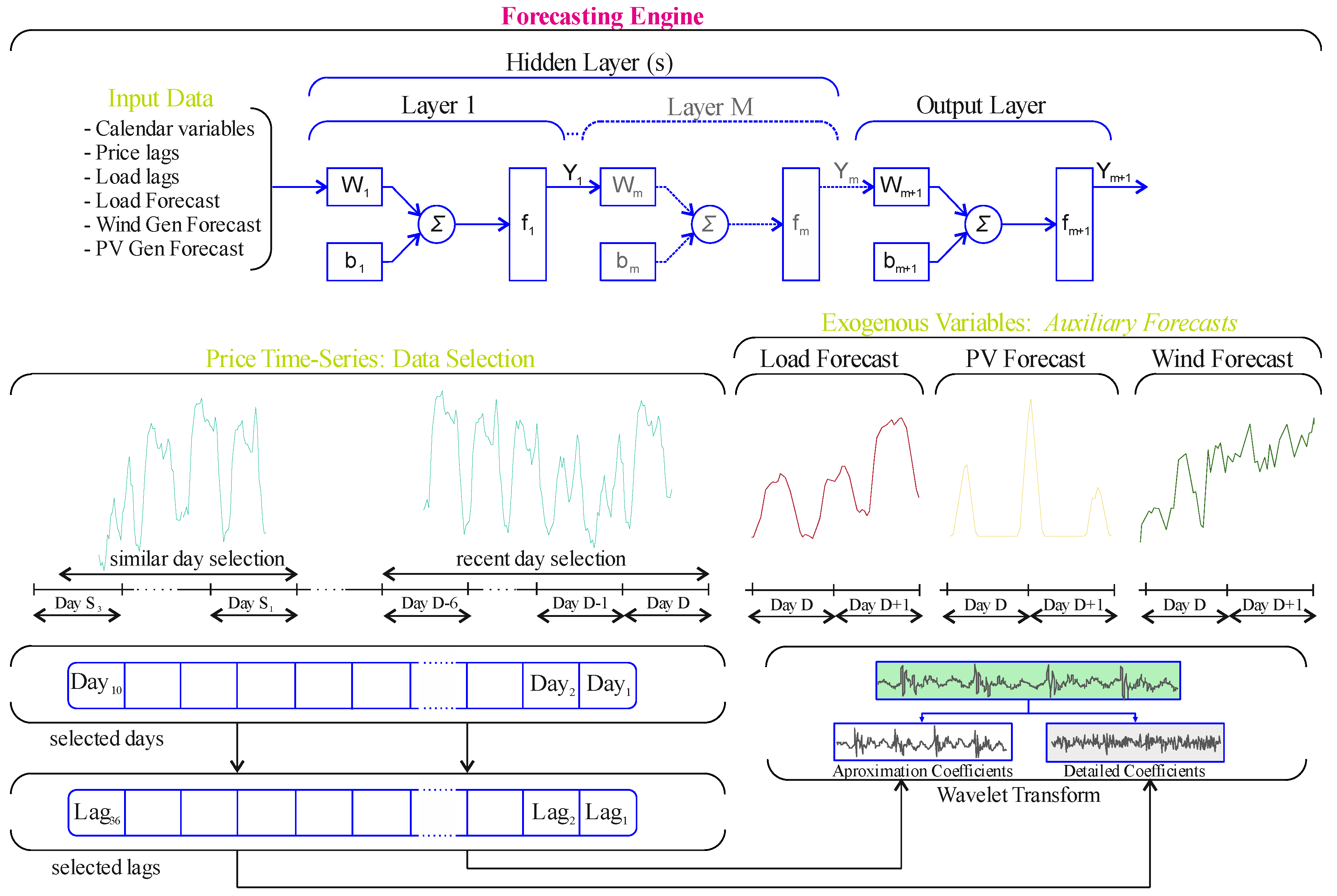
Thus, taking advantage of the knowledge already gathered in [45], an analogous approach was followed, using a FFNN with 2-hidden layers, and an ad-hoc number of neurons. This multi-layer configuration is one of the most common topologies where, in each network layer, every neuron response is given by the activation function evaluation of a cost given by a biased weighted sum, which works as a threshold. For two consecutive layers $\left[l-1,l\right]$ this can be expressed mathematically as follows:

$$y_j=f_j\left({\displaystyle \sum _{i=1}^m{\omega }_{ij}{x}_i+b_j}\right),\forall i\in \left[0,m\right]\wedge j\in \left[0,n\right],$$

(3)

where $m$ is the number of neurons in layer $l-1$ and $n$ is the number of neurons in layer $l$; $y_j$ is the output for neuron $j$ in layer $l$; $f_j$ is the employed activation function; $x_i$ and $b_j$ are input signals; and finally ${\omega }_{ij}$ is the weight of the synaptic connection between neurons $i$ and $j$.

The Scaled Conjugate Gradient Backpropagation (SCG) algorithm is then used as a learning algorithm. The performance of the FFNN is evaluated through the mean absolute error (MAE) at each training step (iteration). Additionally, a standard cross-validation technique (K-fold) was used to partition the data set into 4 mutually exclusive subsets, with a distribution of 75% and 25% of training and validation data, respectively. An extended overview of the described forecasting methodology is presented in Figure 5.

Besides the forecasting engine choice, another delicate issue surrounding forecasting accuracy is the proper feature selection (selected price explanatory variables) [46]. By this means, first a pre-selection stage is carried out where Correlation Analysis (CA) is performed over the available price data, i.e., we take the current day D (last available information) and measure the partial correlation between the prior lags with a span up to a total of 168 h (enabling the capture of intra-day and intra-week relationships), and by selecting the most significant lags the recent days set is formed. Then, a complementary set containing information regarding Similar Days (SD) is also formed, i.e., we take the current day D and find other historical days (SD = 3 days) with a similar daily pattern, thereby exploring the seasonal properties of the electricity price time-series. With this stage completed, then Wavelet Transform is used to decompose the signal up to three levels into its detailed and approximation coefficients, and these are also fed to the multi-layer network.

In addition, the FFNN input layer is completed with a set of exogenous variables, including calendar variables (hour, season, weekday and binary holiday indexes), lagged load and renewable generation, as well as load and renewable generation estimates (i.e., with the same time horizon for which the price forecast is made).

5. Hybrid System Modeling

In this section, the modeling of the several sources and coupling devices that form the HES is presented as realistically as possible. These sources will supply the existing electrical load, and include the battery bank, the pumped-storage hydropower, wind turbine, PV generator, and the power converters. In addition, the grid-connected topology enables the interaction with the upstream grid, which is considered as a perfect power source or sink, i.e., electric power is purchased from upstream grid to supply existing loads and/or charge storage units, otherwise in surplus situations to export (sell) the exceeding power to the upstream grid. The available storage capacity will play a vital role, providing the ability to respond peak time loads and store energy surplus during off-peak periods.

5.1. Kinetic Battery Model (KiBaM)

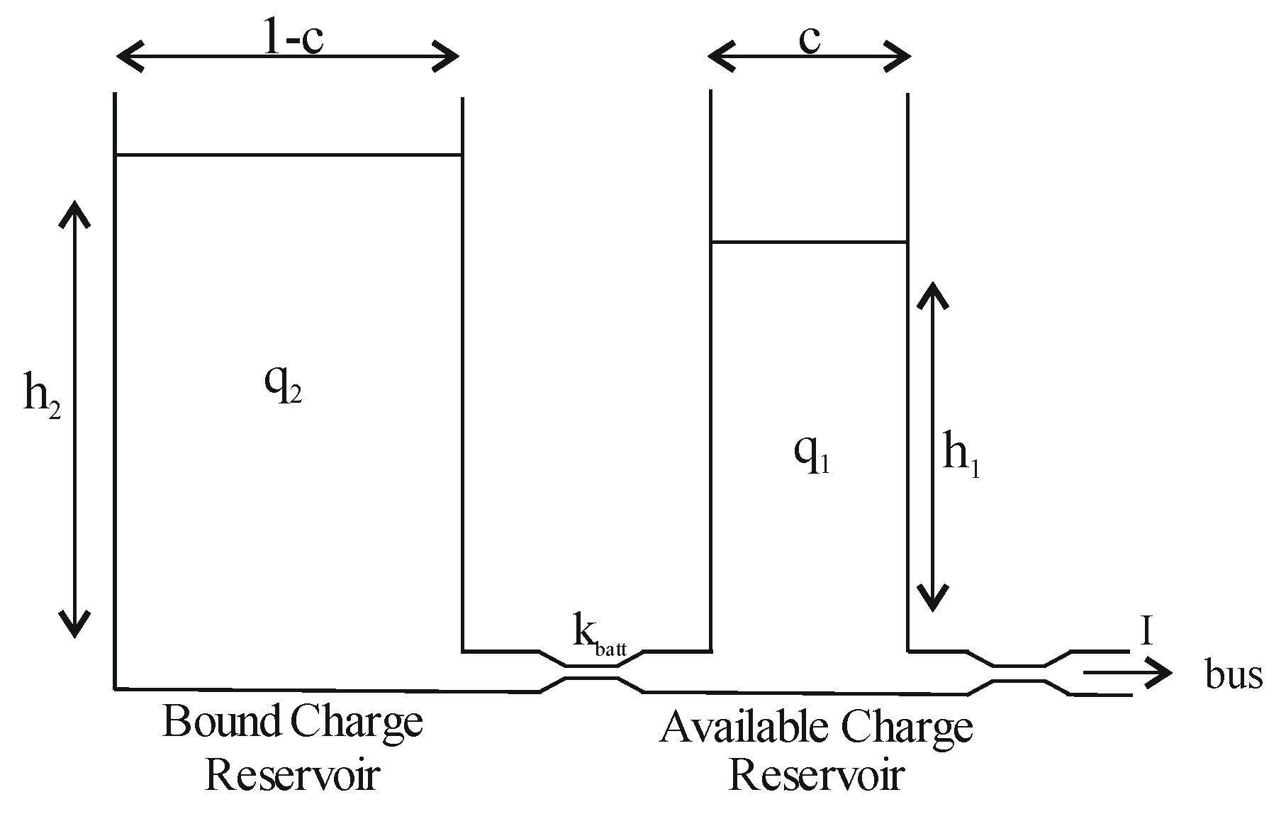
The integration of a battery pack into the HES is highly recommended since it will store the surplus energy and supply the power deficit for the different operation conditions. The literature offers a comprehensive range of models to describe the behavior of different types of batteries under different operating conditions [47,48]. Among them, four major groups stand out: electrochemical, stochastic, electrical and analytical models. In this work, authors employed the powerful and widely used analytical model: Kinetic Battery Model (KiBaM) [49], the same model that is used by the computational tools Homer^® and Hibrid2^®.

KiBaM models the total capacity of a battery in two reservoirs, separated by a conductance, as illustrated in Figure 6. The available charge reservoir contains a fraction $c$ of the total (nominal) capacity q_max (expressed by q₁), responsible for the immediate supply of energy to the connected load. The bound charge reservoir has a fraction $1-c$ of the total capacity (expressed by q₂) and is responsible for supplying energy exclusively to the available charge reservoir. The rate of charge flow between reservoirs depends on the conductance parameter $k_{\mathrm{batt}}$, as well as the difference between the two reservoirs height $\left(h_1-h_2\right)$, with $h_1=q_1/c$ and $h_2=q_2/\left(1-c\right)$. After periods of battery discharge/charge the reservoirs tend to balance, i.e., $h_1=h_2$.

The flows of available and bound charge during a constant current discharge or charge I [A], are computed using the differential equations system, as shown in Equation (4). A full model description, including the maximum allowable battery charge and discharge power equations, as well as the amount of available and bound energy at each time-step can be found in [50,51]. In this work, specific model parameters were identified using the information provided by the manufacturers and are available in

Table 2. KiBaM model: battery bank specifications.

Parameter	Value
$q_{\max }$	131.3305 kWh
$c$	0.6213
$k_{\mathrm{batt}}$	0.185

. The battery bank has a capacity about 5 times larger than a low range electric vehicle battery and is, nowadays, easy to assemble with solutions like Tesla’s^© Powerwall and Powerpack (up to 210 kWh-AC) solutions:

$$\{\begin{array}{c}\frac{d{q}_2}{dt}=k_{\mathrm{batt}}\left(h_1-h_2\right)\\ I=-\frac{d{q}_1}{dt}-\frac{d{q}_2}{dt}\end{array},$$

(4)

At each time-step, the maximum amount of discharge/charge power is computed, as well as the available energy and bound energy and from these two we determine the total amount of energy (storage) $q(t)=q_1(t)+q_2(t)$, to then compute one of the most important battery parameters: its state-of-charge (SOC), $SO{C}_{\mathrm{batt}}\left(t\right)=q\left(t\right)/q_{\max }$.

5.2. Pumped-Storage Hydropower

Hydropower generation with pumping is characterized by the presence of two reservoirs, one upstream and the other downstream. The concept behind this system is simple: in surplus off-peak periods, with a lower energy price, water is pumped upstream, then when the demand is higher (peak periods), and consequently the energy price is higher (more profitable), the stored water is turbinated to produce energy. Given these characteristics, PSH has a very important load balancing role, since it allows a high penetration of intermittent sources.

As defined in the literature [11,52,53,54], the amount of power generated, $P_{\mathrm{hydro}}\left[\mathrm{W}\right]$, and the pumped flow rate, $Q_{\mathrm{pump}}\left[{\mathrm{m}}^3{\mathrm{s}}^{-1}\right]$, can be determined using Equations (5) and (6), respectively:

$$P_{\mathrm{hydro}}={\mathsf{\mu }}_{\mathrm{hydro}}{\mathsf{\rho }}_{\mathrm{water}}g{h}_{\mathrm{net}}{Q}_{\mathrm{turbine}},$$

(5)

$$Q_{\mathrm{pump}}={\mathsf{\mu }}_{\mathrm{pump}}\raisebox{1ex}{$P_{\mathrm{pump}}$}\!\left/ \!\raisebox{-1ex}{${\mathsf{\rho }}_{\mathrm{water}}g{h}_{\mathrm{net}}$}\right.,$$

(6)

where ${\mathsf{\mu }}_{\mathrm{hydro}}[\%]$ and ${\mathsf{\mu }}_{\mathrm{pump}}[\%]$ represent the turbine and pump energy conversion efficiencies, respectively; $h_{\mathrm{net}}\left[\mathrm{m}\right]$ is the effective head; $Q_{\mathrm{turbine}}\left[{\mathrm{m}}^3{\mathrm{s}}^{-1}\right]$ is the turbined water flow; $P_{\mathrm{pump}}\left[\mathrm{W}\right]$ is the pump power consumption; ${\mathsf{\rho }}_{\mathrm{water}}$ is the water density, typically 1000 kg m⁻³ (4 °C); $g$ is the gravitational acceleration, usually 9.81 ms⁻².

Table 3. PSH specifications.

Parameter	Value
$h_{\mathrm{net}}$	25 m
$P_{\mathrm{hydro}\mathrm{installed}}$	150 kW
$V_{\mathrm{total}}$	35,000 m3

displays all the remaining parameters associated with the hydropower turbine application.

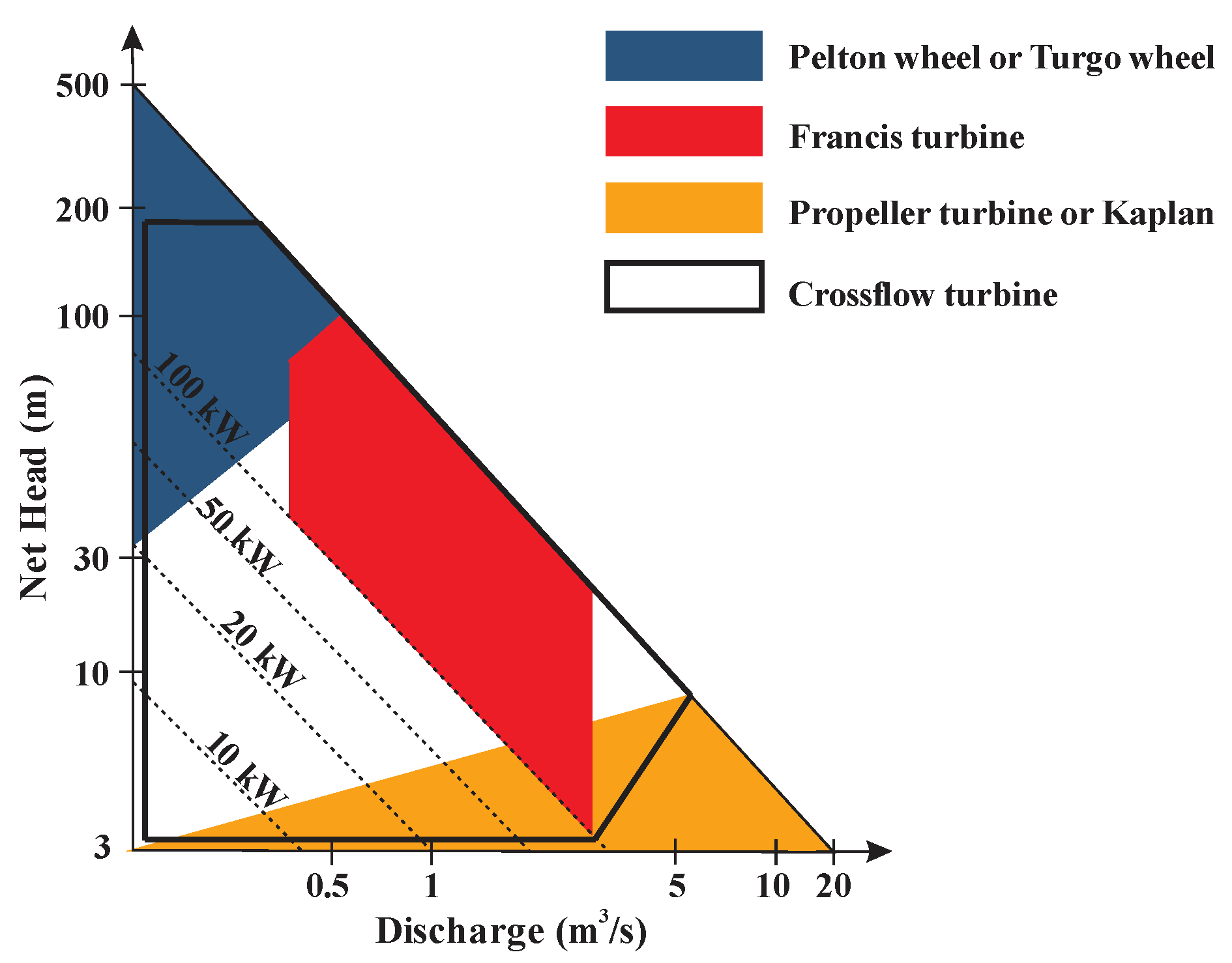
A Francis turbine is a good fit for energy demanding appliances. For this HES a mini hydropower application (<1 MW) is considered, feasible with low to medium head resources with relatively small dams, as Figure 7 reveals. China has exploited these mature small-scale ranges better than anyone else [55], proving the effectiveness of these technologies, leading the charts with around 200 GW of installed hydropower capacity.

Having selected a Francis turbine, and in order to replicate its operational conditions in the best manner, since the output rate depends heavily upon percent of actual flow to nominal flow, instead of using an approximate constant efficiency (such as the euro efficiency standard), it was decided to do the modeling of the performance as a function of the turbine flow, as shown in [57]. For this purpose, a 5th degree polynomial approximation was made to the curve data points, with a R² = 0.9906, resulting in the following polynomial expression:

$${\mathsf{\mu }}_{\mathrm{hydro}}\left(Q\right)=1.19\times {10}^{-10}{Q}^5-6.58\times {10}^{-8}{Q}^4+1.39\times {10}^{-5}{Q}^3-1.4\times {10}^{-3}{Q}^2+0.071Q-0.637,$$

(7)

Additionally, for the sake of simplification $h_{\mathrm{net}}\left[\mathrm{m}\right]$ was considered constant despite the volume change in the reservoir, ${\mathsf{\mu }}_{\mathrm{hydro}}[\%]$ and ${\mathsf{\mu }}_{\mathrm{pump}}[\%]$ were considered equal. Finally, since PSH allows storage in an analogous form as the battery bank, the concept of SOC has also been attributed, and it is computed as the ratio between the current reservoir capacity and its maximum capacity allowance, i.e., $SO{C}_{\mathrm{hydro}}\left(t\right)=V\left(t\right)/V_{\max }$.

5.3. Wind Power Model

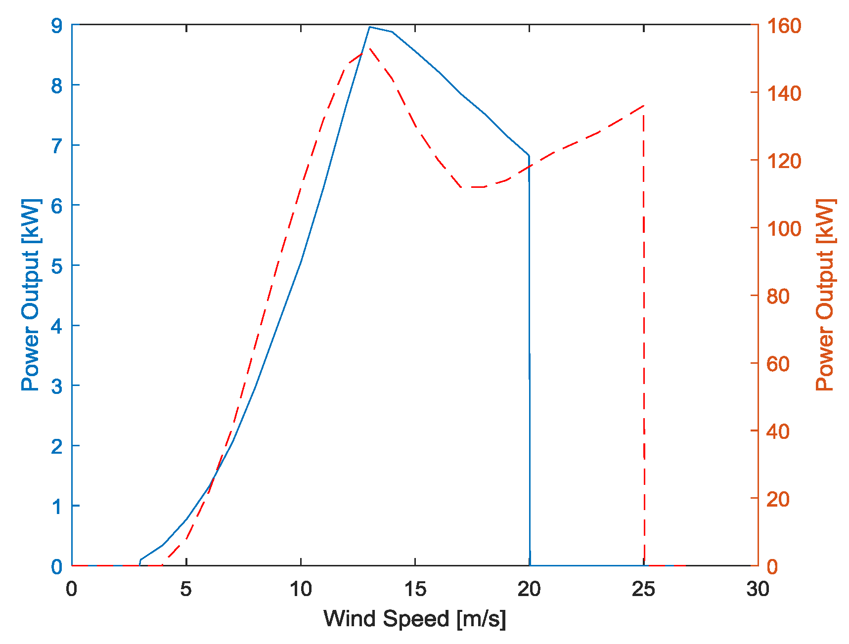
The wind energy conversion process is characterized by two specific curves associated with each wind turbine model. Power output of wind turbine generator at a specific site depends on wind speed at hub height and speed characteristics of the turbine [58], furthermore the wind speed needs to be constrained between a model’s specific cut-in and cut-out speeds. One known as power curve relates the turbine output power with the wind speed, the other is the power efficiency curve relating the turbine output power with the available power in the wind (power coefficient).

In order to perform the wind speed mapping to turbine’s output power $P_{\mathrm{wind}}$, the authors used the approximated power curves provided by the manufacturers, as depicted in Figure 8, despite the existence of linear, nonlinear and physical approximated models [1,51,58,59,60]. In this paper, the adopted wind energy conversion system fell on a combination of Bergey BWC Excel-10 and Norwin 24-STALL-150 kW turbines, in order to a total an exact amount of 200 kW of installed capacity.

Additional details vis-à-vis important features can be seen in

Table 4. Wind Turbine Modelling: Bergey and Norwin.

Parameter	Value	Parameter	Value
$P_{\mathrm{Wind}\mathrm{installed}}$	200 kW	$\mathsf{\alpha }$	1/7
$z_1$	30 m	$z_2$	30 m
$P_{1\mathrm{rated}}$	10 kW	$P_{2\mathrm{rated}}$	150 kW
Cut-in speed	2.5 m/s	Cut-in speed:	4 m/s
Cut-Out speed	20 m/s	Cut-Out speed	25 m/s
# of Turbines	5	# of Turbines	1

. The wind speed measured by the anemometer at a certain height need to be corrected given the wind shear effect; to this end the Power Law Profile was used, Equation (8), with the power law exponent $\mathsf{\alpha }=1/7$:

$$\frac{u}{u_{\mathrm{r}}}={\left(\frac{z}{z_{\mathrm{r}}}\right)}^{\mathsf{\alpha }},$$

(8)

where $u_{\mathrm{r}}\left[m{s}^{-1}\right]$ is the measured (available) wind speed at height $z_{\mathrm{r}}\left[m\right]$ and $u\left[m{s}^{-1}\right]$ is the wind speed at hub height $z\left[m\right]$ of the wind turbine.

5.4. Solar Photovoltaic Model

Solar PV systems generate electric power from solar energy through PV cells. As pointed out in Section 1, substantial penetration levels can be found both in conventional producers’ portfolios, as well as in residential and business/industry appliances, seeking financial savings. To this end, its relatively portable and sizeable structure, the increased technological maturity, hand-in-hand with targeted fiscal policies and other incentives, constituted unparalleled attractiveness factors. As such, it makes it one of the most consensual solutions for hybrid energy systems, with the disadvantage of only being able to operate for 8 h per day.

With this regard, a rich literature is available concerning the accurate behavior mapping of photovoltaic (PV) cells operating under different conditions. Among them we can highlight the commonly used single diode or two diode models, as well as three or more diodes and partial-shading models. However due to the computational effort they require, an alternative followed in HES modeling is to use a more synthesized model [2,12,13]. PV cells are the main units of a PV generator, and are grouped to form panels or arrays.

Considering a PV generator formed by $N_{\mathrm{S}}$ modules connected in series, $N_{\mathrm{P}}$ connected in parallel, with a maximum power point $P_{\mathrm{MPP},\mathrm{STC}}\left[\mathrm{W}\right]$ under STC conditions, i.e., the standard test condition temperature $T_{\mathrm{ref},\mathrm{STC}}$ and with an irradiance $G_{\mathrm{ref},\mathrm{STC}}$, with an efficiency rate ${\mathsf{\mu }}_{\mathrm{MPP}}[\%]$ and a temperature coefficient of the open-circuit voltage ${\mathsf{\alpha }}_{\mathrm{VOC}}\left[\mathrm{V}°{\mathrm{C}}^{-1}\right]$, then for a given solar irradiance $G\left[{\mathrm{Wm}}^{-2}\right]$ the PV generator maximum power output $P_{\mathrm{solar}}\left[\mathrm{W}\right]$ is given by Equation (9) [61]:

$$P_{\mathrm{solar}}={\mathsf{\mu }}_{\mathrm{MPP}}\left(P_{\mathrm{MPP},\mathrm{STC}}\frac{G}{G_{\mathrm{ref},\mathrm{STC}}}\left(1+{\mathsf{\alpha }}_{\mathrm{VOC}}\left(T_{\mathrm{cell}}-T_{\mathrm{ref},\mathrm{STC}}\right)\right)\right)N_{\mathrm{S}}{N}_{\mathrm{P}},$$

(9)

where the cell temperature, Equation (10) is a function of the ambient temperature $T_{\mathrm{amb}}\left[°\mathrm{C}\right]$ and the nominal operating cell temperature $\mathrm{NOCT}\text{}\left[°\mathrm{C}\right]\text{}$ under NOCT conditions i.e., with an air temperature $T_{\mathrm{ref},\mathrm{NOCT}}$ and an irradiance $G_{\mathrm{ref},\mathrm{NOCT}}$:

$$T_{\mathrm{cell}}\left[°\mathrm{C}\right]=T_{\mathrm{amb}}+\frac{G}{G_{\mathrm{ref},\mathrm{NOCT}}}\left(\mathrm{NOCT}-T_{\mathrm{ref},\mathrm{NOCT}}\right),$$

(10)

It is also important to notice that PV systems are commonly coupled with a grid-connected inverter, that besides the DC/AC conversion task, employs an MPP-tracking algorithm to ensure that the maximum power is being extracted (its absence may account for losses up to 30%). The efficiency of these algorithms is nowadays well above 95%, and in this work a value of 99% was assumed, based on the Chint Power^© CPS SC100KT datasheet. Additionally, to achieve a total of 75 kW, the $V_{\mathrm{PM}}$ voltage of each module, as well as the maximum input voltage (DC) of the grid-inverter, 880 V, for the CPS SC100KT, needs to be taken into account, therefore we end up with a configuration with $N_{\mathrm{S}}=28$ and $N_{\mathrm{P}}=9$.

In this paper, for simulation purposes, a HARP^© NU-RD300S monocrystalline silicon photovoltaic module, with an 18.3% conversion efficiency, was employed. The full PV panel specifications are presented

Table 5. Specifications of the PV solar module.

Parameter	Value	Parameter	Value
${\mathsf{\alpha }}_{\mathrm{VOC}}$	−0.0029 V/°C	$T_{\mathrm{ref},\mathrm{NOCT}}$	25 °C
$T_{\mathrm{ref},\mathrm{STC}}$	25 °C	$G_{\mathrm{ref},\mathrm{NOCT}}$	800 W/m2
$G_{\mathrm{ref},\mathrm{STC}}$	1000 W/m2	$P_{\max }$	300 W
$V_{\mathrm{PM}}$	31.2 V	$P_{\mathrm{PV}\mathrm{installed}}$	75 kW
$\mathrm{NOCT}$	49 °C	${\mathsf{\mu }}_{\mathrm{MPP}}$	99%
${\mathsf{\eta }}_{\mathrm{m}}$	18.3%	$V_{\begin{array}{l}\max \left(\mathrm{DC}\right)\\ \mathrm{grid}-\mathrm{inverter}\end{array}}$	880 V
$N_{\mathrm{S}}$	28	$N_{\mathrm{P}}$	9

.

5.5. Diesel Generator

Diesel generators, also known as diesel gensets are a stable and robust option to feed unserved loads, widely used as stand-alone application in isolated areas, especially in developing countries, where India stand outs [62], or in complementary forms, for instance coupled with PV systems and storage, reducing pollution, noise, the partial loads which reduces the already low efficiency of the generator and fuel consumption, which in addition, to direct savings, translates into indirect savings associated with costly diesel fuel transportation, especially in rural areas.

In this work, diesel generators are always seen as a backup option, given its weak thermal efficiency and its pollutant emissions, to ensure the HES supply safety. A linear approximation, Equation (11), frequently used to approximate the amount of fuel the generator consumes, $F_{\mathrm{consumption}}\left[\mathrm{L}{\mathrm{h}}^{-1}\right]$ to generate electricity [16,51]:

$$F_{\mathrm{consumption}}=F_0\times Y_{\mathrm{gen}}+F_1\times P_{\mathrm{gen}},$$

(11)

where $F_0\left[\mathrm{L}{\mathrm{h}}^{-1}{\mathrm{kW}}^{{}^{-1}}\right]$ stands for the fuel curve intercept coefficient, $Y_{\mathrm{gen}}\left[\mathrm{kW}\right]$ for the rated capacity of the generator, $F_1\left[\mathrm{L}{\mathrm{h}}^{-1}{\mathrm{kW}}^{{}^{-1}}\right]$ is the fuel curve slope and $P_{\mathrm{gen}}\left[\mathrm{kW}\right]$ the generator power output. In this context, two diesel generators with a rated power, $Y_{\mathrm{gen}}=60\mathrm{kW}$, more suitable for large energy deficits and one diesel generator with a rated power $Y_{\mathrm{gen}}=12\mathrm{kW}$ for small deviations were integrated on the HES portfolio. To calculate the equation parameters, the approximate fuel consumption data at ¼, ½, ¾ and full load of real generators were used, as illustrated in Figure 9, with the constant parameters defined as: $F_0=0.0481\mathrm{L}{\mathrm{h}}^{-1}{\mathrm{kW}}^{{}^{-1}}$ and $F_1=0.2187\mathrm{L}{\mathrm{h}}^{-1}{\mathrm{kW}}^{{}^{-1}}$ for the 60 kW generator, and $F_0=0.0532\mathrm{L}{\mathrm{h}}^{-1}{\mathrm{kW}}^{{}^{-1}}$ and $F_1=0.2167\mathrm{L}{\mathrm{h}}^{-1}{\mathrm{kW}}^{{}^{-1}}$ for the 12 kW generator.

5.6. Power Electronic Converters

Besides energy generation sources and loads, power electronic converters are fundamental blocks in a HES. The possible configurations of the hybrid system are namely DC coupled, AC coupled and hybrid coupled system [9].

The AC/DC and DC/DC power converters were modeled according to their efficiency. The DC/AC electronic power converter was modeled based on [61], where the converter is characterized according to its efficiency as a function of the normalized rated power, $\frac{P_{\mathrm{in}}}{P_{\mathrm{rated}}}$, expressed by Equation (12), therefore the only input parameter that characterizes the model is the converter rated power:

$${\eta }_{\mathrm{conv}\left(\mathrm{DC}/\mathrm{AC}\right)}[\%]=1-\frac{P_{\mathrm{rated}}}{P_{\mathrm{in}}}\left(0.0094+0.013\left(\frac{P_{\mathrm{in}}}{P_{\mathrm{rated}}}\right)+0.04{\left(\frac{P_{\mathrm{in}}}{P_{\mathrm{rated}}}\right)}^2\right),$$

(12)

With regard to the DC/DC converter, the current high efficiency designs decrease the losses to the extent of achieving efficiencies close to 98/99%, as the bidirectional full SiC 200 kW DC/DC converter efficiency curve shows, therefore a constant value of ${\eta }_{\mathrm{conv}\left(\mathrm{DC}/\mathrm{DC}\right)}=98\%$ was considered reasonable.

6. Results

To validate and analyze the proposed operation dispatch strategy, two different scenarios were considered. In the first, a grid-connected topology that allows exchanges with the upstream grid is considered. These exchanges are governed by the existence of surplus or deficits, then the estimated cost/income obtained by using the grid is evaluated, if surpasses the benefits or the constraints revealed by the different technologies of the hybrid system (expressed by its cost functions, Equations (1) and (2)). Afterwards, a standalone (off-grid) topology is tested, where the diesel generator(s) will supply existing deficits and any generation surplus is now limited only to storage, there being no possibility of sale, as such any surplus that exceeds the storage capacity is considered wasted.

6.1. First Scenario

In the first scenario, the topology enables power-flows with the upstream grid. The same was tested in 4 different situations, which correspond to 1 week per season of the year. The chosen weeks were from February 09th to the 15th of 2016 (winter week); from April 25th to May the 01st of 2016 (spring week); from August 08th to the 14th of 2016 (summer week); finally, from November 11th to the 17th of 2016 (fall week)

Thereby, not only the load profile, the prices and the renewable generation are different, but also the initial SOCs (SOC_batt(0) and SOC_hydro(0)) of storage technologies, i.e., constitute four different starting points, as can be seen in

Table 6. HES Simulation: Main results.

Test Week	SOCbatt(0)	SOChydro(0)	$\overline{\mathsf{\epsilon }}\left(\mathit{k}\right)$	${\overline{\mathit{P}}}_{\mathrm{grid}}$	Gridbuy	Gridsell	SOCbatt (168)	SOChydro (168)
12–18 February (Winter)	0.50	0.99	22.17	17.62	87.11	1.97	0.21	0.25
18–24 May (Spring)	0.85	0.85	−3.82	1.53	31.48	25.62	0.92	0.90
10–16 August (Summer)	0.70	0.50	−8.89	−1.36	24.36	38.51	0.71	0.68
11–17 November (Fall)	0.90	0.75	8.54	8.61	65.61	6.83	0.29	0.24

, where the main simulation results include the average non-dispatchable power balance $\overline{\mathsf{\epsilon }}\left(k\right)$; the average power-flow with the upstream grid ${\overline{P}}_{\mathrm{grid}}$; its respective imports and exports costs Grid_buy and Grid_sell; lastly the final SOCs are presented, (SOC_batt(168) and SOC_hydro(168)). For instance, it makes perfect sense when we refer to the hydro plant to consider the initial SOC in a summer week (SOC_hydro = 0.50) lower than the existing SOC in the winter week (SOC_hydro = 0.99).

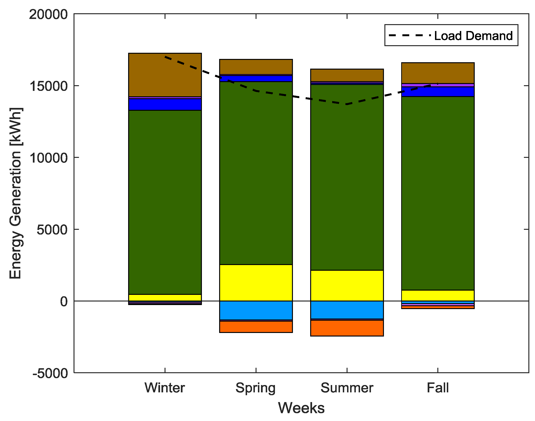
To begin with, we can see the extreme of when there is a week (winter) that presents a very weak renewable generation and high load levels, especially due to the absence of solar generation, as such most of the power flow is given by the upstream grid and the PSH unit, since its initial SOC was practically maximum. Interestingly, the spring week shows that on average the renewable generation slightly exceeds the load by about 4 kW. However, the average price of the exchanges with the grid is slightly positive, proving the balance of the implemented HES dispatch strategy that takes advantage of the existing surplus not only to profit, but also to leveling both SOCs during the 168 h. In turn, the summer week, leveraged by high wind and photovoltaic generation levels, illustrates not only significant net sales, but also enables the upstream pumping to refill partially the dam and the SOC_hydro(168) is 18% higher than the initial one, while the battery bank is used punctually and remains with a relatively unchanged SOC. For the fall week, we can see an average renewable generation deficit, therefore the HES is called upon to alleviate this deficit, and the PSH and grid are responsible for serving the remaining load demand.

Additionally, the resulting energy HES dispatch for these 4 weeks is illustrated by the bar plot in Figure 10, where the share of energy generation (168 h) of each HES technology and its respective load level is represented. As we can see, the employed datasets clearly reveal the benefits of the used hybrid system sizing, with an installed wind power capacity far superior to the remaining generation technologies. Furthermore, the statistics from each test week, i.e., the mean, standard deviation, minimum and maximum value and its mean load value are presented in

Table 7. Test weeks statistics and STPF forecasting performance.

Test Week	Mean	St. Dev	Min	Max	Mean Load	MAPE (%)	RMSE (€)
12–18 February (Winter)	2.45 × 10−2	9.75 × 10−3	2.23 × 10−3	4.65 × 10−2	108.0	9.12	2.53 × 10−3
18–24 May (Spring)	2.66 × 10−2	9.31 × 10−3	2.25 × 10−3	4.23 × 10−2	92.9	6.67	1.73 × 10−3
10–16 August (Summer)	2.69 × 10−2	6.66 × 10−3	1.40 × 10−2	4.00 × 10−2	87.0	5.49	1.89 × 10−3
11–17 November (Fall)	4.06 × 10−2	9.75 × 10−3	1.63 × 10−2	7.58 × 10−2	110.1	6.51	3.67 × 10−3

, side-by-side with the respective forecasting performance, measured by the common MAPE (%) and RMSE metrics.

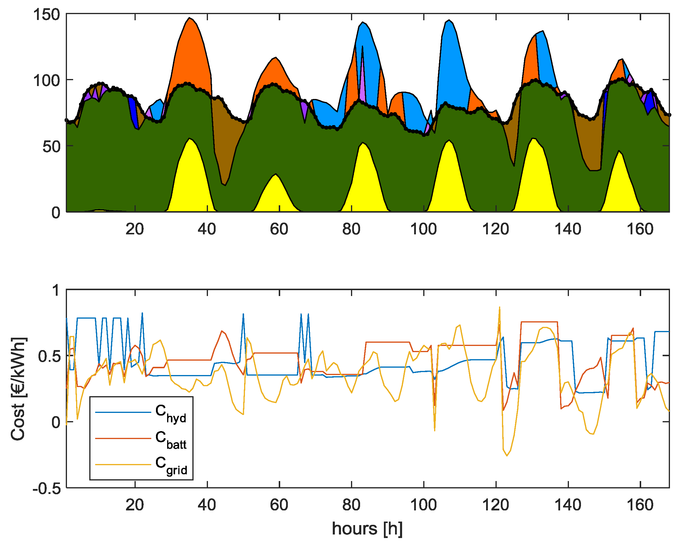
To better understand the followed dispatch strategy, Figure 11 and Figure 12 are presented to better highlight the proposed dispatch strategy, regarding the summer week simulation. Figure 11 illustrates the obtained generation mix profile for 168 h horizon and the cost functions for the hydro, storage bank and grid and, based on these, the cost-effective generation mix for this scenario was determined. As we can observe this scenario presents an approximately constant PV generation and load profile, with the exception of the first day, where the almost null irradiance levels unveil the presence of a cloudy day. The high levels of wind generation can almost exclusively suppress the existing load for many hours, as such it allows to increase the SOC_hydro and sales to the upstream grid. As intended, the battery bank has preferably an upper load balancing role within short periods of time. Moreover when the prices are expected to be low $\left(\widehat{p}\left(k\right)-\frac{1}{24}{\displaystyle {\sum }_{j=1}^{24}{\widehat{p}}_j<0}\right)$ and $\mathsf{\epsilon }\left(k\right)\ge 0$, the strategy favors the energy buying, otherwise, when prices are higher $\left(\widehat{p}\left(k\right)-\frac{1}{24}{\displaystyle {\sum }_{j=1}^{24}{\widehat{p}}_j\ge 0}\right)$ and $\mathsf{\epsilon }\left(k\right)\ge 0$, PSH is dispatched. The plot shows the cost functions for the hydro, storage and grid and, based on these, the cost-effective generation mix for this scenario was determined.

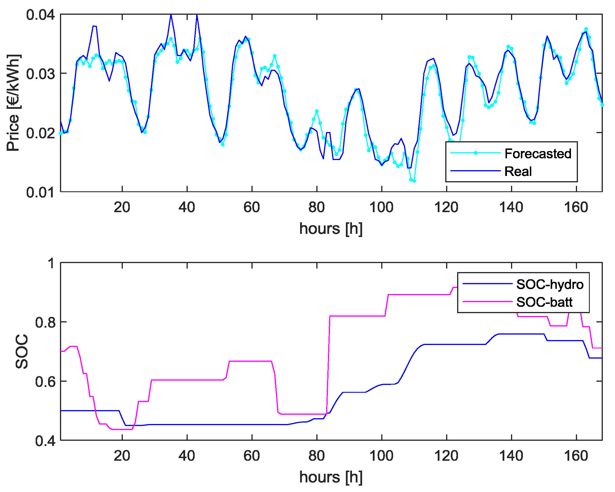
In turn, the one day-ahead electricity prices forecast for this summer week (10–16 August) with an average daily MAPE of 5.49%., as well as the SOCs profile during the 168 h, can be seen in Figure 12. Being evident that there is a surplus that allows the storage systems charging, and uncovers the intended tendency of the proposed strategy, in doing so in periods where low electricity prices are expected, as is the case with the abrupt SOC ramping around hour 80 h, in a clear contrast with what happens for instance in the first few hours of the simulation.

6.2. Second Scenario

For the second scenario a standalone off-grid topology is considered in the same simulation weeks, where diesel generators are called to respond when it is not viable using the hybrid system. To implement this scenario, some modifications in Algorithm need to be accounted, where the cost function is re-written as: $\min \left\{\begin{array}{c}{C}_{\mathrm{solar}}{P}_{\mathrm{solar}}\left(k\right)+C_{\mathrm{wind}}{P}_{\mathrm{wind}}\left(k\right)+C_{\mathrm{diesel}}\left(k\right)P_{\mathrm{diesel}}\left(k\right)\\ +{\displaystyle {\sum }_{j=1}^2{C}_j\left(SO{C}_j\left(k\right),\Delta SO{C}_j\right)P{g}_j}\end{array}\right\}$; where the diesel cost, $C_{\mathrm{diesel}}$, is given by an exponential decay function, $C_{\mathrm{diesel}}\left(k\right)=P_{\mathrm{Diesel}}{e}^{-\left(1-\max \left\{SO{C}_1(k)SO{C}_2(k)\right\}\right)}$ if $\mathsf{\epsilon }\left(k\right)>0$, whereas for $\mathsf{\epsilon }\left(k\right)\le 0$ the considered dispatch cost is irrelevant, since boundary conditions (system constraints) are unidirectionally limited, i.e., one way power flow (bus injection); the power balance equation is re-written as $P_{\mathrm{solar}}\left(k\right)+P_{\mathrm{wind}}\left(k\right)+{\displaystyle {\sum }_{j=1}^{2}P{g}_j\left(k\right)+P_{\mathrm{diesel}}\left(k\right)=P_{\mathrm{D}}\left(k\right)}$; and the systems constraints concerning the diesel generator are $P_{\mathrm{diesel}\mathrm{gen}}>0$, if $\mathsf{\epsilon }\left(k\right)>0$; else $P_{\mathrm{diesel}\mathrm{gen}}=0$, since it does not have the capacity to absorb situations of surplus energy, therefore non-dispatchable energy could be wasted. Finally, the generators must operate between its capacity limits $P_{\mathrm{diesel},\min }\le P_{\mathrm{diesel}}\left(k\right)\le P_{\mathrm{diesel},\max }$. The same test weeks were considered for testing purposes, and the main simulation results for this topology are presented in

Table 8. HES Simulation: Main results.

Test Week	SOCbatt(0)	SOChydro(0)	$\overline{\mathsf{\epsilon }}\left(\mathit{k}\right)$	${\overline{\mathit{P}}}_{\mathbf{diesel}}$	Dieselcost	SOCbatt (168)	SOChydro (168)
12–18 February (Winter)	0.50	0.99	22.17	15.38	703.17	0.17	0.15
18–24 May (Spring)	0.85	0.85	−3.82	3.03	137.20	0.64	0.49
10–16 August (Summer)	0.70	0.50	−8.89	0.87	47.19	0.40	0.49
11–17 November (Fall)	0.90	0.75	8.54	13.71	631.68	0.50	0.21

, and by analyzing them we can see that a standalone topology can be implemented as a backup option for potential power shortages. Though, it compares badly with the grid-connected topology of the first scenario, demonstrating how expensive diesel systems are nowadays and how more demanding they are from the PSH and the battery bank (increased discharge cycles and DOD).

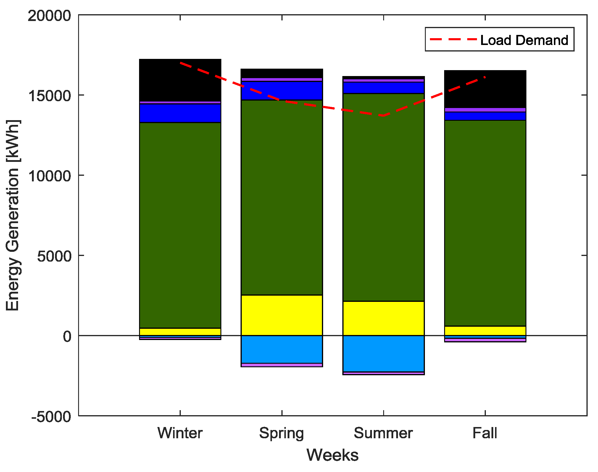
Moreover, the resulting energy HES dispatch for these four weeks is illustrated by the bar plot in Figure 13, where the share of energy generation (168 h) of each HES technology and its respective load level is represented. We can see a similar pattern to the one in Figure 10, since the non-dispatchable generation is the same; however, in a stand-alone application the energy storage technologies serve an increased share of load demand, namely the PSH. Last but not least, it was possible to infer that for the summer week, using relatively high initial SOC values with continuous periods of energy surplus, gave rise to curtailment situations, i.e., energy was dumped, however only for very sporadic time-steps, thus validating the compromise made when sizing the battery bank.

7. Conclusions

This manuscript provides a new operation strategy to cope with the challenges and opportunities of integrating solar PV, wind energy, given its intermittent nature, with hydropower and storage units for electricity generation, in a grid-connected system. By integrating energy resources into an optimum arrangement, the variability nature of solar and wind resources can be partially compensated, and the overall system becomes more reliable and cost-effective.

Short term price forecasting in deregulated electricity markets is a major research topic, with a large profusion of published techniques, since accurate forecasting methodologies have the utmost importance as decision-making tools for market players. The authors, using an experience capital, employed a forecasting engine based on a feed-forward neural network preceded by an improved input selection stage. This preprocessing stage not only relies on a similar/recent days selection mechanism, but also employs WT with filtering purposes, in order to feed the best input information as possible. Gains from the forecasting accuracy will translate into a better “informed” dispatch and consequently increase the HES profitability.

The mix of generation technologies resulting from the proposed operation strategy and the performed forecasting, as described in the algorithm, showed good performances, using the available information to drive the best dispatch decisions. The battery bank and the PSH dam have been able to accumulate the excess power generated by the HES and supply it to the system load during the hybrid power shortage, depending on the electricity prices forecast.

Therefore, the PV-wind-hydro with storage capabilities both from the increasingly cheaper storage banks and also of the PSH, which despite its significant presence in the grid, has not been incorporated frequently in this type of studies, is widely recommended and can also be used for remote areas. The proposed strategy has been tested in simulation under different scenarios for a week horizon and revealed a balanced dispatch strategy for a small range prosumer with a rich energy generation portfolio, working as effectively for energy surplus or deficit situations. Simulations revealed that very low irradiation levels can strongly condition the HES, since the wind despite its unstable nature constitutes itself as the predominant energy source. This fact is not unrelated to the chosen sizing, making evident the need for complementary strategies for systems with high levels of renewable penetration. The simulation with the off-grid system for exceptional situations has revealed that the use of diesel generators is a limited but a safe option, and for a better functioning it requires a greater storage capacity since it cannot be called for surplus situations.

Future works will consider additional costs, the importance of a more accurate prediction model to improve the algorithm’s decision-making process, the increase in the forecast time horizon and additional simulation scenarios.

References

- Potli, M.; Mallikarjuna, A.; Balachandra, J.C.; Venugopal, N. Optimal Sizing of Wind/Solar/Hydro in an Isolated Power System using SMFFT based Cuckoo Search Algorithm. In Proceedings of the 2016 IEEE 6th International Conference on Power Systems (ICPS), New Delhi, India, 4–6 March 2016; IEEE: New Delhi, India, 2016. [Google Scholar]
- Upadhyay, S.; Sharma, M.P. Development of hybrid energy system with cycle charging strategy using particle swarm optimization for a remote area in India. Renew. Energy 2015, 77, 586–598. [Google Scholar] [CrossRef]
- Nojavan, S.; Majidi, M.; Zare, K. Performance improvement of a battery/PV/fuel cell/grid hybrid energy system considering load uncertainty modeling using IGDT. Energy Convers. Manag. 2017, 147, 29–39. [Google Scholar] [CrossRef]
- Arsalis, A.; Georghiou, G.E. A Decentralized, Hybrid Photovoltaic-Solid Oxide Fuel Cell System for Application to a Commercial Building. Energies 2018, 11, 3512. [Google Scholar] [CrossRef]
- Scientist, N. Record Amounts of Renewable Energy Added to the Mix in 2016. Available online: https://www.newscientist.com/article/2127056-record-amounts-of-renewable-energy-added-to-the-mix-in-2016/ (accessed on 29 December 2017).
- IRENA. Renewable Capacity Statistics 2018; International Renewable Energy Agency (IRENA): Abu Dhabi, Arab, 2018. [Google Scholar]
- Schopfer, S.; Tiefenbeck, V.; Staake, T. Economic assessment of photovoltaic battery systems based on household load profiles. Appl. Energy 2018, 223, 229–248. [Google Scholar] [CrossRef]
- Upadhyay, S.; Sharma, M.P. A review on configurations, control and sizing methodologies of hybrid energy systems. Renew. Sustain. Energy Rev. 2014, 38, 47–63. [Google Scholar] [CrossRef]
- Shivarama Krishna, K.; Sathish Kumar, K. A review on hybrid renewable energy systems. Renew. Sustain. Energy Rev. 2015, 52, 907–916. [Google Scholar] [CrossRef]
- Bento, P.; Nunes, H.; Pombo, J.; Mariano, S.; Calado, M.d.R. Daily Operation Optimization for Grid-Connected Hybrid System Considering Short-Term Electricity Price Forecast Scheme. In Proceedings of the 2018 IEEE International Conference on Environment and Electrical Engineering and 2018 IEEE Industrial and Commercial Power Systems Europe (EEEIC / I&CPS Europe), Palermo, Italy, 12–15 June 2018; pp. 1–6. [Google Scholar]
- Ma, T.; Yang, H.; Lu, L.; Peng, J. Technical feasibility study on a standalone hybrid solar-wind system with pumped hydro storage for a remote island in Hong Kong. Renew. Energy 2014, 69, 7–15. [Google Scholar] [CrossRef]
- Xu, L.; Ruan, X.; Mao, C.; Zhang, B.; Luo, Y. An improved optimal sizing method for wind-solar-battery hybrid power system. IEEE Trans. Sustain. Energy 2013, 4, 774–785. [Google Scholar]
- Malheiro, A.; Castro, P.M.; Lima, R.M.; Estanqueiro, A. Integrated sizing and scheduling of wind/PV/diesel/battery isolated systems. Renew. Energy 2015, 83, 646–657. [Google Scholar] [CrossRef] [Green Version]
- Reddy, S.S. Optimal scheduling of thermal-wind-solar power system with storage. Renew. Energy 2017, 101, 1357–1368. [Google Scholar] [CrossRef]
- Kong, W.; Dong, Z.Y.; Hill, D.J.; Luo, F.; Xu, Y. Short-Term Residential Load Forecasting based on Resident Behaviour Learning. IEEE Trans. Power Syst. 2017, 33, 1087–1088. [Google Scholar] [CrossRef]
- Lu, J.; Wang, W.; Zhang, Y.; Cheng, S. Multi-objective optimal design of stand-alone hybrid energy system using entropy weight method based on HOMER. Energies 2017, 10, 1664. [Google Scholar] [CrossRef]
- An, L.; Tuan, T. Dynamic Programming for Optimal Energy Management of Hybrid Wind–PV–Diesel–Battery. Energies 2018, 11, 3039. [Google Scholar] [CrossRef]
- Sanchez, V.M.; Chavez-Ramirez, A.U.; Duron-Torres, S.M.; Hernandez, J.; Arriaga, L.G.; Ramirez, J.M. Techno-economical optimization based on swarm intelligence algorithm for a stand-alone wind-photovoltaic-hydrogen power system at south-east region of Mexico. Int. J. Hydrogen Energy 2014, 39, 16646–16655. [Google Scholar] [CrossRef]
- Oviroh, P.O.; Jen, T.C. The energy cost analysis of hybrid systems and diesel generators in powering selected base transceiver station locations in Nigeria. Energies 2018, 11, 7–9. [Google Scholar]
- Fodhil, F.; Hamidat, A.; Nadjemi, O. Potential, optimization and sensitivity analysis of photovoltaic-diesel-battery hybrid energy system for rural electrification in Algeria. Energy 2019, 169, 613–624. [Google Scholar] [CrossRef]
- Zheng, J.H.; Chen, J.J.; Wu, Q.H.; Jing, Z.X. Multi-objective optimization and decision making for power dispatch of a large-scale integrated energy system with distributed DHCs embedded. Appl. Energy 2015, 154, 369–379. [Google Scholar] [CrossRef]
- Dong, W.; Li, Y.; Xiang, J. Optimal sizing of a stand-alone hybrid power system based on battery/hydrogen with an improved ant colony optimization. Energies 2016, 9, 785. [Google Scholar] [CrossRef]
- Khare, V.; Nema, S.; Baredar, P. Solar-wind hybrid renewable energy system: A review. Renew. Sustain. Energy Rev. 2016, 58, 23–33. [Google Scholar] [CrossRef]
- Yamamoto, S.; Park, J.-S.; Takata, M.; Sasaki, K.; Hashimoto, T. Basic study on the prediction of solar irradiation and its application to photovoltaic-diesel hybrid generation system. Sol. Energy Mater. Sol. Cells 2003, 75, 577–584. [Google Scholar] [CrossRef]
- Lujano-Rojas, J.M.; Monteiro, C.; Dufo-López, R.; Bernal-Agustín, J.L. Optimum load management strategy for wind/diesel/battery hybrid power systems. Renew. Energy 2012, 44, 288–295. [Google Scholar] [CrossRef]
- Šajn, N. Electricity “Prosumers”; European Parliamentary Research Service (EPRS): Brussels, Belgium, 2016. [Google Scholar]
- Kästel, P.; Gilroy-Scott, B. Economics of pooling small local electricity prosumers—LCOE & self-consumption. Renew. Sustain. Energy Rev. 2015, 51, 718–729. [Google Scholar]
- Chitsaz, H.; Zamani-Dehkordi, P.; Zareipour, H.; Parikh, P.P. Electricity price forecasting for operational scheduling of behind-the-meter storage systems. IEEE Trans. Smart Grid 2018, 9, 6612–6622. [Google Scholar] [CrossRef]
- Neon; Technical University of Berlin; ETH Zürich. DIW Berlin Open Power System Data. Available online: https://open-power-system-data.org/ (accessed on 15 November 2018).
- Statista Prices of dDiesel Fuel in Czechia 2004–2018. Available online: https://www.statista.com/statistics/603765/diesel-fuel-prices-czech-republic/ (accessed on 19 November 2018).
- British Government Department (HM Treasury). Red Diesel: Call for Evidence. Available online: https://www.gov.uk/government/consultations/red-diesel-call-for-evidence/red-diesel-call-for-evidence (accessed on 21 February 2019).
- OECD Taxing Energy Use 2018: Companion to the Taxing Energy Use Database; OECD Publishing: Paris, France, 2018; ISBN 9789264289437.
- Singh, N.; Husain, S.; Mohanty, S.R. An improved WNN for day-ahead electricity price forecasting. 4th Stud. Conf. Eng. Syst. SCES 2015 2016, 1–6. [Google Scholar]
- Foruzan, E.; Scott, S.D.; Lin, J. A comparative study of different machine learning methods for electricity prices forecasting of an electricity market. 2015 N. Am. Power Symp. NAPS 2015 2015, 1–6. [Google Scholar]
- Catalão, J.P.S.; Mariano, S.J.P.S.; Mendes, V.M.F.; Ferreira, L.A.F.M. Short-term electricity prices forecasting in a competitive market: A neural network approach. Electr. Power Syst. Res. 2007, 77, 1297–1304. [Google Scholar] [CrossRef] [Green Version]
- Eurostat Electricity Price Statistics; Eurostat: Luxembourg, 2018.
- Sánchez, A.A.; Nieta, D.; González, V.; Contreras, J. Portfolio Decision of Short-Term Electricity Forecasted Prices through Stochastic Programming. Energies 2016, 1–19. [Google Scholar]
- Nowotarski, J.; Weron, R. Recent advances in electricity price forecasting: A review of probabilistic forecasting. Renew. Sustain. Energy Rev. 2018, 81, 1548–1568. [Google Scholar] [CrossRef]
- González, J.P.; Roque, A.M.S.; Pérez, E.A. Forecasting functional time series with a new hilbertian ARMAX model: Application to electricity price forecasting. IEEE Trans. Power Syst. 2018, 33, 545–556. [Google Scholar] [CrossRef]
- Monteiro, C.; Ramirez-Rosado, I.J.; Fernandez-Jimenez, L.A.; Ribeiro, M. New probabilistic price forecasting models: Application to the Iberian electricity market. Int. J. Electr. Power Energy Syst. 2018, 103, 483–496. [Google Scholar] [CrossRef]
- Wang, F.; Li, K.; Zhou, L.; Ren, H.; Contreras, J.; Shafie-khah, M.; Catalão, J.P.S. Daily pattern prediction based classification modeling approach for day-ahead electricity price forecasting. Int. J. Electr. Power Energy Syst. 2019, 105, 529–540. [Google Scholar] [CrossRef]
- Monteiro, C.; Ramirez-Rosado, I.J.; Fernandez-Jimenez, L.A.; Conde, P. Short-term price forecasting models based on artificial neural networks for intraday sessions in the Iberian electricity market. Energies 2016, 9, 721. [Google Scholar] [CrossRef]
- Alamaniotis, M.; Bargiotas, D.; Bourbakis, N.G.; Tsoukalas, L.H. Genetic Optimal Regression of Relevance Vector Machines for Electricity Pricing Signal Forecasting in Smart Grids. IEEE Trans. Smart Grid 2015, 6, 2997–3005. [Google Scholar] [CrossRef]
- Ghasemi, A.; Shayeghi, H.; Moradzadeh, M.; Nooshyar, M. A novel hybrid algorithm for electricity price and load forecasting in smart grids with demand-side management. Appl. Energy 2016, 177, 40–59. [Google Scholar] [CrossRef]
- Bento, P.M.R.; Pombo, J.A.N.; Calado, M.R.A.; Mariano, S.J.P.S. A bat optimized neural network and wavelet transform approach for short-term price forecasting. Appl. Energy 2018, 210, 88–97. [Google Scholar] [CrossRef]
- Uniejewski, B.; Weron, R. Efficient forecasting of electricity spot prices with expert and LASSO models. Energies 2018, 11, 2039. [Google Scholar] [CrossRef]
- Zhang, C.; Li, K.; Mcloone, S.; Yang, Z. Battery Modelling Methods for Electric Vehicles—A Review. Eur. Control Conf. 2014, 2673–2678. [Google Scholar]
- Jongerden, M.R.; Haverkort, B.R. Battery Modeling; Faculty of Electrical Engineering, Mathematics and Computer Science, University of Twente: Enschede, The Netherlands, 2008. [Google Scholar]
- Yurur, O.; Liu, C.H.; Moreno, W. Modeling battery behavior on sensory operations for context-aware smartphone sensing. Sensors (Switzerland) 2015, 15, 12323–12341. [Google Scholar] [CrossRef] [PubMed]
- Manwell, J.F.; McGowan, J.G. Lead acid battery storage model for hybrid energy systems. Sol. Energy 1993, 50, 399–405. [Google Scholar] [CrossRef]
- Mandal, S.; Das, B.K.; Hoque, N. Optimum sizing of a stand-alone hybrid energy system for rural electrification in Bangladesh. J. Clean. Prod. 2018, 200, 12–27. [Google Scholar] [CrossRef]
- Papaefthymiou, S.V.; Karamanou, E.G.; Papathanassiou, S. a.; Papadopoulos, M.P. A wind-hydro-pumped storage station leading to high RES penetration in the autonomous island system of Ikaria. IEEE Trans. Sustain. Energy 2010, 1, 163–172. [Google Scholar] [CrossRef]
- McLean, E.; Kearney, D. An evaluation of seawater pumped hydro storage for regulating the export of renewable energy to the national grid. Energy Procedia 2014, 46, 152–160. [Google Scholar] [CrossRef]
- Ma, T.; Yang, H.; Lu, L.; Peng, J. Pumped storage-based standalone photovoltaic power generation system: Modeling and techno-economic optimization. Appl. Energy 2014, 137, 649–659. [Google Scholar] [CrossRef]
- International Renewable Energy Agency (IRENA). Hydropower; International Renewable Energy Agency (IRENA): Abu Dhabi, Arab, 2012; Volume 1. [Google Scholar]
- Razak, J.; Ali, Y.; Alghoul, M. Application of crossflow turbine in off-grid pico hydro renewable energy system. Recent Adv. Appl. Math. 2010, 519–526. [Google Scholar]
- Kaunda, C.S.; Kimambo, C.Z.; Nielsen, T.K. Potential of Small-Scale Hydropower for Electricity Generation in Sub-Saharan Africa. ISRN Renew. Energy 2012, 2012, 1–15. [Google Scholar] [CrossRef] [Green Version]
- Bhandari, B.; Lee, K.-T.; Cho, Y.-M.; Ahn, S.-H. Optimization of Hybrid Renewable Energy Power system: A review. Int. J. Precis. Eng. Manuf. Technol. 2015, 2, 99–112. [Google Scholar] [CrossRef]
- Allali, K.; Azzag, E.B.; Kahoul, N. Wind-diesel hybrid power system integration in the South Algeria. Front. Energy 2015, 9, 259–271. [Google Scholar] [CrossRef]
- Bencherif, M.; Brahmi, B.N.; Chikhaoui, A. Optimum Selection of Wind Turbines. Sci. J. Energy Eng. 2014, 2, 36. [Google Scholar] [CrossRef] [Green Version]
- Riffonneau, Y.; Bacha, S.; Barruel, F.; Ploix, S. Optimal Power Flow Management for Grid Connected PV Systems With Batteries. IEEE Trans. Sustain. Energy 2011, 2, 309–320. [Google Scholar] [CrossRef]
- Saurav, K.; Bansal, H.; Nawhal, M.; Chandan, V.; Arya, V. Minimizing energy costs of commercial buildings in developing countries. 2016 IEEE Int. Conf. Smart Grid Commun. SmartGridComm 2016, 2016, 637–642. [Google Scholar]
Figure 1.
Schematic representation of the proposed hybrid system architecture.
Figure 2.
Equation (2) codomain illustration: PSH and battery bank costs for four different SOCs.
Figure 3.
Market Electricity Prices (OTE) and Prosumer’s Load Profile.
Figure 4.
Weather Data: Wind Speed, Solar Irradiance and Temperature.
Figure 5.
Illustration of the employed price forecasting: FFNN input data selection mechanism.
Figure 6.
The two-well kinetic battery model (KiBaM).
Figure 7.
Head-flow ranges of small hydro turbines [56].
Figure 8.
Wind Turbines Power Curves: BWC Excel-10 (blue line) and Norwin 24-STALL-150 (dashed red line).
Figure 9.
Diesel Generator: Fuel Consumption Curves as a function of Power Output.
Figure 10.
Energy generation share and load levels for each week. Where yellow, green and blue represent the PV, wind and hydro generation, respectively, light blue represents pumping periods, brown buying periods and orange selling periods. In turn, purple represents discharge periods, and lilac periods of charging the battery bank.
Figure 11.
Dispatched energy mix and its dispatch costs for the summer week. Where yellow, green and blue represent the PV, wind and hydro generation, respectively, light blue represents pumping periods, brown buying periods and orange selling periods. In turn, purple represents discharge periods, and lilac periods of charging the battery bank. Black represents the existing load level.
Figure 12.
Price Forecast vs. Real Prices and State of Charge evolution for the summer week.
Figure 13.
Energy generation share and load levels for each week. Where yellow, green and blue represent the PV, wind and hydro generation, respectively, light blue represents pumping periods, black for diesel generation periods. In turn, purple represents discharge periods, and lilac periods of charging the battery bank.