A Power Converter Decoupled from the Resonant Network for Wireless Inductive Coupling Power Transfer

1
Department of Instrumental and Electrical Engineering, Xiamen University, Xiamen 361005, China
2
Department of Biological System Engineering, Washington State University, Pullman, WA 99164, USA
3
Fujian Collaborative Innovation Center for R&D of Coach and Special Vehicle, Xiamen 361024, China
4
Fujian Key Laboratory of Advanced Design and Manufacture for Bus$Coach, Xiamen 361024, China
5
School of Mechanical and Electrical Engineering, Guizhou Normal University, Guiyang 550001, Guizhou, China
*
Author to whom correspondence should be addressed.
Energies 2019, 12(7), 1192; https://doi.org/10.3390/en12071192
Submission received: 13 February 2019
/
Revised: 22 March 2019
/
Accepted: 22 March 2019
/
Published: 27 March 2019
Abstract
:In a traditional inductive coupling power transfer (ICPT) system, the converter and the resonant network are strongly coupled. Since the coupling coefficient and the parameters of the resonant network usually vary, the resonant network easily detunes, and the system efficiency, power source capacity, power control, and soft switching conditions of the ICPT system are considerably affected. This paper presents an ICPT system based on a power converter decoupled from the resonant network. In the proposed system, the primary inductor is disconnected from the resonant network during the energy injection stage. After storing a certain amount of energy, the primary inductor is reconnects with the resonant network. Through this method, the converter can be decoupled from the resonant network, and the resonant network can be tuned under various coupling coefficients. Theoretical analysis was explored first. Simulations and experimental work are carried out to verify the theoretical analysis. The results show that the proposed ICPT system has the virtues of low power source capacity, independent power control, and soft switching operation under different coupling coefficients.
1. Introduction
Since the late 2000s, inductive coupling power transfer (ICPT) has been widely used for wireless energy transmission over large air gaps [1,2,3,4,5]. Due to its safety and convenience, ICPT is a promising method for charging electrical vehicles (EVs) [6,7]. However, during the charging process, the ICPT system faces problems such as the varying load from the changed state of charge (SOC) of the batteries [8], coil misalignment [9], and the varying air gap, either of which will lead to changes in the electromagnetic characteristics and coefficients [6,10]. All these issues can be attributed to the problem caused by changes in the coupling coefficient, which should be considered in the design of an ICPT system.
To achieve optimal output power and efficiency, it is necessary to adjust the frequency of the power converter, according to the changes in the system parameters [11,12,13]. Many impedance reconfiguration methods have been introduced for frequency tracking in ICPT [14,15,16,17]. Hsu and Hu [15] adopted an LCL structure with a variable inductance. By changing the value of the variable inductance, the ICPT system was retuned. In Kamineni et al. [16], a switchable bank of capacitors consisting of four capacitors with a ratio of 1:2:4:8 was employed, producing 16 different capacitance combinations to adjust the frequency.
Using a phase-locked loop (PLL) and by tracking the zero-phase angle of the voltage and current, the ICPT system could automatically track the optimal frequency [18,19,20]. Matysik [18] introduced the application of a phase controller that can adjust the phase shift of the current and voltage in a resonant tank with no periodic voltage waveform. Gati et al. [19] employed a digital PLL to decrease the phase shift between the secondary current and the inverter output voltage by adjusting the inverter frequency.
By using a self-oscillating switching technique in the control of the inverter, output controllability, dynamic response, and self-adaptability can also be improved [21,22,23]. In Xu et al. [21], by detecting the zero-crossing point of secondary current, a series–series converter was used to automatically adjust the frequency and obtain better self-adaptability under different air gaps. Namadmalan et al. [22] applied a one-third clock divider behind the zero-crossing comparator. The system was able to switch between fundamental and third-harmonic modes for different load and coupling conditions.
As a strong coupling exists between the power source, the converter, and the resonant tank, the traditional ICPT system is a high-order system. The transient process involved in this type of system is usually complex and hard to analyze [24]. Based on a separated energy injection and free oscillation strategy [24,25], the power source can be decoupled from the resonant tank during a free oscillation period. However, the coupling between the power supply and the resonant tank still exists in the energy injection period.
Li et al. [25] provided an energy injection and free oscillation strategy for a direct AC–AC converter. When the converter is in a resonance state, the resonant tank is completely isolated from the power source and the system can be described as a second-order system. However, in their system, the energy injection can only start at the positive zero-crossing moment of the primary current in each half-cycle. Therefore, an integrated control method [26] should be used to control the switches of the converter. The integrated control method needs complex control circuit and control process, which is difficult to apply in practical applications.
Power control plays an important role in the ICPT system [27]. Traditional power control methods include phase shifting, frequency control, and reactive power control. These power control methods, however, may result in an increase in switching losses and electromagnetic noise due to the difficulty for switching devices to be always turned on and off at zero current point [28,29]. The energy injection and free oscillation strategy control the power by using the cycle number of the injected energy under a resonant state, and the converter drives a purely resistive load. All switching devices in this strategy operate under zero-current switching conditions [24,25]. This strategy can solve the problems caused by the traditional power control methods. However, in an energy injection and free oscillation ICPT system, the resonant tank cannot be decoupled from the converter during the energy injection period. Therefore the converter frequency should be the same as the resonant frequency. In practical applications, when the coupling coefficient and load changed, the system will detune, and the reflected impedance from the secondary part may be reactive, which make the equivalent primary impedance complex [24]. The converter must drive an additional reactance. And the converter cannot inject energy efficiently in the positive half cycle, which complicates power control in practical applications.
This paper presents an ICPT system with a two-stage energy injection and self-tuning (TSEIST) control strategy. In the proposed system, the primary inductor is disconnected with the resonant network and connected with the power source in the energy injection stage. In the self-tuning stage, the primary inductor is reconnected with the resonant network for self-tuning. As such, the power converter can be completely decoupled from the resonant network and independently inject energy into the primary inductor. Since the energy injection is independent, the converter frequency need not be the same as the resonant tank frequency, and the power can be controlled independently. In the TSEIST ICPT system, the power can be controlled only by the energy injection time. Compared with traditional tuning methods, this method reduces the difficulties of power control.
In a traditional system, to ensure soft switching conditions, it is necessary to use complex control circuits, such as zero-crossing switching or an integrated control method. In the proposed system, switching time margins are applied to ensure soft switching conditions. The time margins allow the switch operations acted within a time period, but not at a time moment, which reduces the switching control difficulty and the circuit complexity. Thus, in the TSEIST ICPT system, the system can be tuned under various coupling coefficients.
2. Basic Structure and System Modeling
2.1. Structure of the TSEIST ICPT System
An AC-DC converter system using an energy injection and free oscillation strategy is shown in Figure 1a [26]. According to the polarity of the input voltage, switch S1 or S2 is turned on for energy injection. The bidirectional switches S3 and S4 are turned on during the free oscillation stage. Note that switches S3 and S4 should not be turned on simultaneously with S1 and S2 in case of a short circuit. The resonant tank is on the right part of the circuit, in which Cp is the tank capacitor, Lp is the primary inductor and Zr is the impedance reflected from the secondary to the primary part. A strong coupling exists between the resonant tank and the converter during the energy injection period. In this system, when reactive components are involved in the reflected impedance, the converter will not effectively inject energy.
A topology of the proposed TSEIST ICPT system is shown in Figure 1b. It consists of a power source UDC, a loosely coupled transformer T (L1 is the primary inductor and L2 is the secondary inductor), a resonant capacitor Cp, two double-throw switches (K1, K2), and the load resistance R. The mutual inductance of the loosely coupled transformer is M.
Different from the traditional ICPT system, the TSEIST ICPT system is based on the double-throw switches, K1 and K2. When K1 is connected to A1 and K2 is connected to B1, the primary inductor L1 is connected to the power source, and the system is in the energy injection stage. When K1 is connected to A2 and K2 is connected to B2, the primary inductor L1 is connected to the resonant capacitor Cp, and the system is in the free oscillation stage. Under this strategy, Lp is connected to the power source only during the energy injection stage, and the converter is completely decoupled from the resonant tank. According to the connection states of K1 and K2, the TSEIST system can work in three stages:
- (1)
- Energy injection stage. In this stage, K1 and K2 connect to A1 and B1, respectively. UDC is connected to L1 and injects energy into the primary coil. In this process, part of the energy is transferred to the secondary coil.
- (2)
- Self-tuning stage. In this stage, K1 and K2 connect to A2 and B2, respectively. Cp is connected to L1 to form a resonant tank and the system begins to resonate. The energy continues to be transferred to the secondary coil.
- (3)
- Shutdown stage. K1 and K2 are switched to the center point, where UDC, Cp, and L1 are isolated from each other. In this stage, the system stops transferring energy to the secondary part and the remaining energy is stored in the capacitor Cp as electrical energy.
In real applications, skipping the shutdown stage is desirable to enhance the output power. In that case, the proposed converter becomes a two-stage converter.
2.2. System Modeling
2.2.1. Energy Injection Stage
In this stage, the system can be described as a first-order system and can be simplified as shown in Figure 2a, where N1 and N2 are the turns of the primary and the secondary coil, respectively; L1 is the primary inductance; and L2 is the secondary inductance. The loosely coupled transformer can be equivalent to a T model circuit, as shown in Figure 2b.
In Figure 2b, Lp is the primary leakage inductance; Ls is the secondary leakage inductance; and Lm is the magnetizing inductance. For simplicity, in this paper, N1 = N2 and L1 = L2 = L. The coupling coefficient k is defined as k = M × (L1 × L2)−1/2. Then, we obtain:
2.2.2. Self-Tuning Stage
In this stage, the loosely coupled transformer is equivalent to the M model as in Figure 3a, and the primary loop impedance can be obtained as:
where ω is the resonant frequency.
The real part is the equivalent load and can be expressed as RC. Thus:
The imaginary part is the total reactance of the system. It contains the primary reactance of inductance L1 and the reactance reflected from secondary inductance L2. Thus:
3. TSEIST Converter
3.1. Topology of the TSEIST Converter
The TSEIST converter structure is shown in Figure 4. The converter consists of a modified H bridge. S1 and S2 correspond to the top switch of the lead bridge. S3 corresponds to the down switch of the lead bridge. S4 and S5 correspond to the top switch of lag bridge. And S6 corresponds to the down switch of the lag bridge. The primary inductor L1 is connected to points A and B of the modified H bridge. Switches S1, S2, S4, and S5 construct a sub-H bridge, which plays the roles of K1 and K2 in Figure 1b. The tank capacitance Cp is connected to points C and D in the sub-H bridge. By controlling the switches S2 and S5, Cp can be connected or disconnected to L1.
In Figure 4, a controller is needed to control the switches S1–6. A voltage sensor is in parallel with Cp to measure the voltage ucp. A current sensor is in series with L1 to measure the current ip. The signals obtained from the sensors are sent to the controller. The controller creates a control strategy to switch the system within the three stages described above.
3.2. State Analysis
The working process of the proposed power converter can be divided into positive and reverse energy transmission periods, which can be further divided into 10 working states, including 6 main states and 4 transitional states, as shown in Figure 5. For clarity, in Figure 5, the loosely coupled transformer T and the load resistor R in Figure 4 are replaced by LC and RC, respectively, as shown in Figure 3b. The states are continuously numbered and illustrated with schematic circuits. The on-state switching devices and branches are denoted with bold solid black lines. The off-state switching devices and branches are denoted with dotted lines. The directions of currents and the polarities of the voltages are also shown in the figure.
The waveforms of the converter are shown in Figure 6 with the state numbers. State ⑩ is the shutdown state of the previous period. S1–6 are all turned off, and no energy is transmitted to the secondary. State ① is identical to the energy injection stage. S1, S2, and S6 are turned on, and UDC is connected to L1. The current ip increases nearly linearly, and energy is injected into the primary coil. The equivalent circuit in this state is shown in Figure 2b. Thus:
Assuming t0 = 0, with the boundary conditions ip (0) = im (0) = is (0) = 0 and Equation (1), we obtain:
where α = R/(1 − k)2L, α is the attenuation factor that expresses the energy consumption of the load. Assuming τ1 = t1 − t0, the primary current ip at the end of this state can be written as:
State ② is a transitional state where the converter switches from the energy injection stage to the self-tuning stage. Compared with state ①, S1 and S6 are turned off in this state. Therefore, ip flows to Cp through D5 instead; UDC stops working; and the energy stored in Cp in the previous cycle is added into this cycle. Compared with state ③, S5 has to be turned on to ensure ip flows bi-directionally to allow the system to enter state ③. Since ip continues to flow forward before the T2 moment, D5 is turned on. Thus, the time period [t1, T2] is defined as a time margin Tm1 for turning on S5. In this interval, S5 is under a soft switching condition.
State ③ is the self-tuning stage. At the t2 moment, S5 is turned on in soft switching, and ip flows bi-directionally. In this stage, the system begins to self-tune and the energy continues to transmit to the secondary coil. As the energy is consumed, the amplitude of ucp decreases exponentially. The duration of this state is related to the coupling coefficient k. The detailed analysis about the self-tuning time is discussed in Section 3.3. Since both magnetic energy and electric energy exist in this period, a transitional state is needed following state ③.
State ④ is a transitional state between the self-tuning stage and the shutdown stage. within this state, S5 is turned off; Cp is charged through S2 and D5; and the magnetic energy in LC is converted into the electric energy in Cp. The system exits from the self-tuning stage after the T4 moment, and the remaining energy in the tank is stored in Cp. Similarly, since ip keeps flowing forward in the interval [T3, T4], D5 is turned on, and the interval is defined as a time margin Tm2 for turning off S5 under the soft switching condition.
The voltage equation in time interval [t1, t4] is:
To solve Equation (8), the boundary conditions should be determined. For convenience, t1 is defined as 0, and thus and = / according to Figure 3b, Figure 5 and Figure 6. Equation (8) can be solved as:
where:
The resonant frequency ω can be simplified to .
State ⑤ is the shutdown stage. In this stage, S1–6 are all switched off. The remaining energy is stored in the capacitor Cp, and thus ip = 0 and ucp = −UDC.
In states ⑥–⑩, the system works similarly as in states ①–⑤, except that the directions of the voltages and currents are in reverse, which will therefore not be explained again.
3.3. Calculation of the Self-Tuning Maintenance Time
Because of the low coupling coefficient, the energy injected into the primary coil cannot be transferred to the secondary coil in one resonant cycle. As shown in Figure 6, the self-tuning stage is maintained for around three cycles. The self-tuning maintenance time varies with the coupling coefficient k.
To calculate the self-tuning maintenance time, the voltage waveform of Cp in the positive energy transmission period is drawn and shown in Figure 7. To show the waveform with complete cycles, the missing parts of the sinusoidal waveform are shown in bold dash line. Here, UE is the amplitude of the decayed sinusoidal voltage ucp, TC is the period of the sinusoidal wave, α1 is the decay factor, and UDC is the voltage of ucp at the end of the self-tuning period.
3.3.1. Number of Resonance Cycles
As shown in Figure 7, ucp is a decayed sinusoid curve with an envelope line . Based on Equation (9), we obtain:
and:
where [.] is the integer function. Note that the number of the resonance cycles must be an integer.
3.3.2. Leading Angle Tβγ
The leading angle Tβγ is related to β and γ, and can be calculated by Equation (10). Thus:
The self-tuning period time should be:
3.3.3. Time Margin for State Change
As T2 is the first zero point of ip, Tm1 can be calculated by Equation (9):
Thus:
3.4. Power Control
From Equation (6), when the energy injection stage ends, the magnetic energy in the primary coil can be expressed as:
The second item can be ignored compared to the first item; thus:
where Wm(τ1) is the energy that should be transmitted in the positive energy transmission period T. The power of the converter is:
Equation (20) shows that the power can be controlled by controlling the energy injection period τ1.
3.5. Transistor Control Strategy Design
3.5.1. Switch Control Function for the Self-Tuning Period
During the self-tuning period, there is a key moment to exit the self-tuning stage. The key moment is determined by the situation of ip, ucp, and whether the energy transfer period is positive or negative. The variables Im, Um, and Pm are defined as situation parameters, which can be generated as a binary signal. Thus:
so, the actual situation of the system can be described by the situation function D:
where “” indicates a non-operation. The D function determines when the system exits the self-tuning resonance. Here, Dp is the exit condition for the positive period and Dr denotes for the negative period.
3.5.2. Control Logic Block and Control Strategy
The block diagram of the control logic is shown in Figure 8. It is composed of the voltage processing unit, current processing unit, and program processor of STM32. In Figure 8, τ1 is the variable that controls the output power, and τ3 is the variable that controls the shutdown duration, which can be canceled as needed. The voltage signal and the current signal from the sensors are sent to the voltage and current processing units to determine the variables Um and Im according to Equation (21). In the control logic software unit, a Pm counter is set for the variable Pm. According to the variables Im, Um, and Pm, the D function calculation unit calculates the value of the situation function D according to Equation (22).
The control strategy generates the control signals g1–6, according to the states in Section 3.2., step-by-step to control the switches. The state duration time Δti (i = 0, 1, 2, 3, 4) is determined by τ1, τ3, Tm1, Tm2, and D, as shown in Table 1. The control strategy is a repetitive state transition loop under the control of the STM32 processor.
4. Experimental Prototype Design
To verify our theoretical analysis of the TSEIST system, a prototype was built for experimental verification.
4.1. Magneto-Electric System Design
As shown in Figure 9, two rectangular pads (460 mm × 370 mm) were designed for primary and secondary coil pads, with a base layer, a ferrite core layer, and a copper coil layer. An organic glass layer was stuck onto the coil for protection. The primary coil had 43 turns, and the turn ratio of the coils was 1:1. The other parameters are listed in Table 2.
4.2. Power Converter
5. Experimental Verification
5.1. Characteristics of the TSEIST ICPT System
A simulation was conducted using SABER and several experiments were completed under the condition of τ1 = 50 μs, τ3 = 50 μs, and k = 0.5. The simulation and experimental results are shown in Figure 12a,b, respectively. The results agreed well with the analysis in Figure 6.
In the experimental results, we found that the bus current iB and the primary current ip increase linearly in the energy injection stage τ1, which shows that the primary inductor is completely decoupled from the resonant tank. The power source injects energy into the primary inductor independently, which coincides with our theoretical analysis. The bus current iB only exists during the energy injection period τ1. This means that UDC injects energy only during the energy injection period, without energy backflow, reducing the capacity of the power source. More than two cycles of ip and ucp occur in the self-tuning period. Compared with iB, the frequency of the resonant tank is about three times greater than that of the power converter. This shows that the proposed converter can operate at a lower switching frequency than the resonance tank frequency, which can reduce the switching loss.
5.2. Power Control
The power can be controlled by the energy injection period τ1. A comparison between the theoretical and experimental power results is provided in Figure 13. The theoretical results were calculated in MATLAB based on Equations (5)–(20). In Equation (20), T was determined as T = τ1 + τ2 + τ3. As τ1 increases from 25 to 45 μs, the theoretical power increases from 65 to 210 W and the experimental power increases from 59 to 199 W. The experimental curve is slightly lower than the calculated curve. This may be due to the coil resistance being ignored in the calculation process.
The experimental results show that, unlike other power control methods, the TSEIST system can control the power easily through the energy injection time.
5.3. Resonant Frequency
The theoretical and experimental results of the frequency are shown in Figure 14. As k changed from 0.1 to 0.4, the theoretical and experimental resonant frequencies changed from 9.77 kHz to 10.6 kHz, and 9.1 kHz to 10 kHz, respectively. The experimental curve is some lower than the calculated curve.
5.4. Soft Switching
The driving voltages, voltage drops and currents of switches S1, S2, and S3, are shown in Figure 15. As shown in Figure 15a, at the point when the driving voltage g1 (the blue curve) jumped upward, the current is1 (the red curve) is zero. S1 is turned on under the ZCS condition. At the point when g1 jumps downward, the voltage uds1 (the yellow curve) of S1 is zero. S1 is turned off under the ZVS condition.
The operation of S2 is more complicated. It is switched twice during a working period, as shown in Figure 15b. When the voltage g2 (the blue curve) jumped upward at the first time, uds2 (green curve) is zero, and S2 is turned on in ZVS. When g2 jumped downward at the first time, the uds2 is zero as well and S2 is turned off in ZVS. When g2 jumped upward at the second time, the current is2 (in red curve) is zero, and S2 is turned on in ZCS. When g2 jumped downward at the second time, uds2 and is2 are both zero, and S2 is turned off in ZVS and ZCS.
In Figure 15b, the time margin Tm1 corresponds to state ⑦ in Figure 5 and interval [t1, T2] in Figure 6. Tm2 corresponds to state ⑨ in Figure 5 and the interval [T3, T4] in Figure 6. In these time margins, D2 is in the “on” state, and S2 is under the ZVS condition. The time margins allow the switches to be turned on or off within a time period, but not at a critical time moment, which coincides with the theoretical analysis.
As shown in Figure 15c, at the point when the driving voltage g3 (the blue curve) jumped upward, S3 is turned on in ZCS. At the point when g3 jumped downward, the voltage uds3 (the yellow curve) of S3 is zero and S3 is turned off in ZVS. The operating waves of S4, S5, and S6 are similar to S1, S2, and S3, respectively.
5.5. Power and Efficiency
The efficiency of the magneto-electric system is related to the coupling coefficient, copper resistance, core loss, and other factors [30]. As this research only evaluates the characteristics of the power converter, the efficiency of the magneto-electric system is not considered. Pin, Pop, Pos, ηp, and ηs are shown in Table 4, in which Pin is the input power, Pop is the output power of power supply (measured at the input of the primary pad), Pos is the output power (measured at the output of the secondary coil), ηp is the efficiency of the power convertor that is derived from Pop divided by Pin, and ηs is the total efficiency, which is derived from Pos divided by Pin and contains the efficiency of the magneto-electric system. For comparison, the input power Pin was all set as 350 W. The data were measured using a power analyzer (WT500, Yokogawa Co., Tokyo, Japan).
In Table 4, the converter efficiency ηp is maintained at a high level and decreases slightly with a decreasing coupling coefficient. The high efficiency may be due to switches working under soft switching conditions, the converter frequency lower than the resonant frequency, and no backflow current to the source. The total efficiency ηs is also higher, but decreases apparently with the decrease in the coupling coefficient. When k = 0.5, ηs is 93.6%, and when k = 0.1, ηs is 89.6%. This phenomenon can be explained by the fact that as the coupling coefficient decreases, the transmission efficiency of the magneto-electric system decreases, resulting in a decrease in the overall efficiency.
6. Conclusions
In this paper, a TSEIST power converter was proposed and theoretically analyzed. In the proposed power converter system, the primary inductor is separated from the resonant tank in the energy injection stage, and the power source is isolated from the resonant tank during the self-tuning stage. Therefore, in this system, the converter is decoupled from the resonant tank and the resonant tank can automatically track the resonant frequency. The converter can operate at a lower switching frequency than the resonance tank frequency, reducing the switching loss. In this system, switching time margins were applied to ensure all switches in the converter operate under soft switching conditions, reducing the complexity of the switch control strategy and the switching losses. Since the energy injection stage can be independently controlled, the output power of the power converter can be easily controlled. On the other hand, as the system avoids energy backflow and the energy injection period varies with the self-tuning period, the input power is automatically adjusted with the coupling coefficient, and the power capacity rating of the converter is reduced to a low level. Simulations were done to verify the theoretical analysis first. And a prototype of an ICPT system with a TSEIST power converter was designed and fabricated to verify the theoretical and simulation results. The experimental results show that the prototyped ICPT system can work at a high efficiency within a large range of coupling coefficients.
Author Contributions
conceptualization, L.C.; methodology, L.C.; software, J.H.; validation, L.C., J.H. and W.W.; formal analysis, W.C., J.H. and M.G.; investigation, L.C., J.H. and W.W.; resources, W.C. and M.G.; data curation, L.C., J.H. and M.G.; writing—original draft preparation, L.C.; writing—review and editing, M.G.; visualization, M.G.; supervision, W.C.; project administration, W.C.; funding acquisition, W.C.
Funding
This research was funded by National Natural Science Foundation of China (NSFC), grant number 51777177; NSFC grant number 51707168; Key Projects of Fujian Collaborative Innovation Center for R&D of Coach and Special Vehicle, grant number 2016AYF002; and Guizhou Science and Technology Department, grant number LKS[2011]19.
Conflicts of Interest
The authors declare no conflict of interest.
References
- Wu, H.H.; Gilchrist, A.; Sealy, K.D.; Bronson, D. A High Efficiency 5 kW Inductive Charger for EVs Using Dual Side Control. IEEE Trans. Ind. Inform. 2012, 8, 585–595. [Google Scholar] [CrossRef] [Green Version]
- García, X.T.; Vázquez, J.; Roncero-Sánchez, P. Design, Implementation Issues and Performance of an Inductive Power Transfer System for Electric Vehicle Chargers with Series–series Compensation. IET Power Electron. 2015, 8, 1920–1930. [Google Scholar] [CrossRef]
- Lu, Y.; Ma, D.B. Wireless Power Transfer System Architectures for Portable or Implantable Applications. Energies 2016, 9, 1087. [Google Scholar] [CrossRef]
- Jiang, C.; Chau, K.T.; Liu, C.; Lee, C.H.T. An Overview of Resonant Circuits for Wireless Power Transfer. Energies 2017, 10, 894. [Google Scholar] [CrossRef]
- Kim, C.G.; Seo, D.H.; You, J.S.; Park, J.H.; Cho, B.H. Design of a Contactless Battery Charger for Cellular Phone. IEEE Trans. Ind. Electron. 2001, 48, 1238–1247. [Google Scholar] [CrossRef]
- Ibrahim, M.; Pichon, L.; Bernard, L.; Razek, A.; Houivet, J.; Cayol, O. Advanced Modeling of a 2-kw Series-series Resonating Inductive Charger for Real Electric Vehicle. IEEE Trans. Veh. Technol. 2015, 64, 421–430. [Google Scholar] [CrossRef]
- Hwang, K.; Cho, J.; Kim, D.; Park, J.; Kwon, J.H.; Kwak, S.I.; Park, H.H.; Ahn, S. An Autonomous Coil Alignment System for the Dynamic Wireless Charging of Electric Vehicles to Minimize Lateral Misalignment. Energies 2017, 10, 315. [Google Scholar] [CrossRef]
- Lin, X.; Stefanopoulou, A.G.; Li, Y.; Anderson, R.D. State of Charge Imbalance Estimation for Battery Strings Under Reduced Voltage Sensing. IEEE Trans. Control Syst. Technol. 2015, 23, 1052–1062. [Google Scholar] [CrossRef]
- Boys, J.T.; Covic, G.A.; Green, A.W. Stability and Control of Inductively Coupled Power Transfer Systems. IEEE Proc. Electr. Power Appl. 2000, 147, 37–43. [Google Scholar] [CrossRef]
- Acero, J.; Carretero, C.; Lope, I.; Alonso, R.; Lucia, Ó.; Burdio, J.M. Analysis of the Mutual Inductance of Planar-Lumped Inductive Power Transfer Systems. IEEE Trans. Ind. Electron. 2013, 60, 410–420. [Google Scholar] [CrossRef]
- Yang, D.; Ren, J.; Liu, D.; Hu, P. Tuning of Mid-range Wireless Power Transfer System Based on Delay-iteration Method. IET Power Electron. 2016, 9, 1563–1570. [Google Scholar] [CrossRef]
- Villa, J.L.; Sallan, J.; Osorio, J.F.S.; Llombart, A. High-Misalignment Tolerant Compensation Topology for ICPT Systems. IEEE Trans. Ind. Electron. 2012, 59, 945–951. [Google Scholar] [CrossRef]
- Zheng, C.; Ma, H.; Lai, J.S.; Zhang, L. Design Considerations to Reduce Gap Variation and Misalignment Effects for the Inductive Power Transfer System. IEEE Trans. Power Electron. 2015, 30, 6108–6119. [Google Scholar] [CrossRef]
- Do-Hyeon, K.; Dukju, A. Self-tuning LCC Inverter Using PWM-Controlled Switched Capacitor for Inductive Wireless Power Transfer. IEEE Trans. Ind. Electron. 2018, 66, 3983–3992. [Google Scholar] [CrossRef]
- Hsu, J.U.W.; Hu, A.P. Determining the Variable Inductance Range for an LCL Wireless Power Pick-up. In Proceedings of the 2007 IEEE Conference on Electron Devices and Solid-State Circuits, Tainan, China, 20–22 December 2007; pp. 489–492. [Google Scholar] [CrossRef]
- Kamineni, A.; Covic, G.A.; Boys, J.T. Self-Tuning Power Supply for Inductive Charging. IEEE Trans. Power Electron. 2017, 32, 3467–3479. [Google Scholar] [CrossRef]
- Kennedy, H.; Bodnar, R.; Lee, T.; Redman-White, W. A Self-Tuning Resonant-Inductive-Link Transmit Driver Using Quadrature Symmetric Delay Trimmable Phase-Switched Fractional Capacitance. IEEE J. Solid-State Circuits 2018, 53, 1694–1707. [Google Scholar] [CrossRef]
- Matysik, J.T. The Current and Voltage Phase Shift Regulation in Resonant Converters with Integration Control. IEEE Trans. Ind. Electron. 2007, 54, 1240–1242. [Google Scholar] [CrossRef]
- Gati, E.; Kampitsis, G.; Manias, S. Variable Frequency Controller for Inductive Power Transfer in Dynamic Conditions. IEEE Trans. Power Electron. 2017, 32, 1684–1696. [Google Scholar] [CrossRef]
- Gati, E.; Kampitsis, G.; Stavropoulos, I.; Papathanassiou, S.; Manias, S. Wireless Phase—Locked Loop Control for Inductive Power Transfer Systems. In Proceedings of the IEEE Applied Power Electronics Conference and Exposition (APEC), Charlotte, NC, USA, 15–19 March 2015; pp. 1601–1607. [Google Scholar] [CrossRef]
- Xu, L.; Chen, Q.; Ren, X.; Wong, S.C.; Tse, C.K. Self-Oscillating Resonant Converter with Contactless Power Transfer and Integrated Current Sensing Transformer. IEEE Trans. Power Electron. 2016, 32, 4839–4851. [Google Scholar] [CrossRef]
- Namadmalan, A. Self-Oscillating Tuning Loops for Series Resonant Inductive Power Transfer Systems. IEEE Trans. Power Electron. 2016, 31, 7320–7327. [Google Scholar] [CrossRef]
- Yan, K.; Chen, Q.; Hou, J.; Ren, X.; Ruan, X. Self-Oscillating Contactless Resonant Converter with Phase Detection Contactless Current Transformer. IEEE Trans. Power Electron. 2014, 29, 4438–4449. [Google Scholar] [CrossRef]
- Li, H.L.; Hu, A.P.; Covic, G.A. Development of a Discrete Energy Injection Inverter for Contactless Power Transfer. In Proceedings of the 2008 3rd IEEE Conference on Industrial Electronics and Applications, Singapore, 3–5 June 2008; pp. 1757–1761. [Google Scholar] [CrossRef]
- Li, H.L.; Hu, A.P.; Covic, G.A. A Direct AC–AC Converter for Inductive Power-Transfer Systems. IEEE Trans. Power Electron. 2012, 27, 661–668. [Google Scholar] [CrossRef]
- Matysik, J.T. A New Method of Integration Control with Instantaneous Current Monitoring for Class D Series-Resonant Converter. IEEE Trans. Ind. Electron. 2006, 53, 1564–1576. [Google Scholar] [CrossRef]
- Moghaddami, M.; Sundararajan, A.; Sarwat, A.I. A Power-Frequency Controller with Resonance Frequency Tracking Capability for Inductive Power Transfer Systems. IEEE Trans. Ind. Appl. 2018, 54, 1773–1783. [Google Scholar] [CrossRef]
- Dede, E.J. Improving the Efficiency of IGBT Series-resonant Inverters using Pulse Density Modulation. IEEE Trans. Ind. Electron. 2011, 58, 979–987. [Google Scholar] [CrossRef]
- Fujita, H.; Akagi, H. Pulse-density-modulated Power Control of a 4 kw, 450 kHz Voltage-source Inverter for Induction Melting Applications. IEEE Trans. Ind. Appl. 1996, 32, 279–286. [Google Scholar] [CrossRef]
- Lin, F.Y.; Covic, G.A.; Boys, J.T. Evaluation of Magnetic Pad Sizes and Topologies for Electric Vehicle Charging. IEEE Trans. Power Electron. 2015, 30, 6391–6407. [Google Scholar] [CrossRef]
Figure 1.
Comparison of two topologies: (a) the energy injection and free oscillation system [26]; (b) the proposed two-stage energy injection and self-tuning (TSEIST) inductive coupling power transfer (ICPT) system.
Figure 1.
Comparison of two topologies: (a) the energy injection and free oscillation system [26]; (b) the proposed two-stage energy injection and self-tuning (TSEIST) inductive coupling power transfer (ICPT) system.
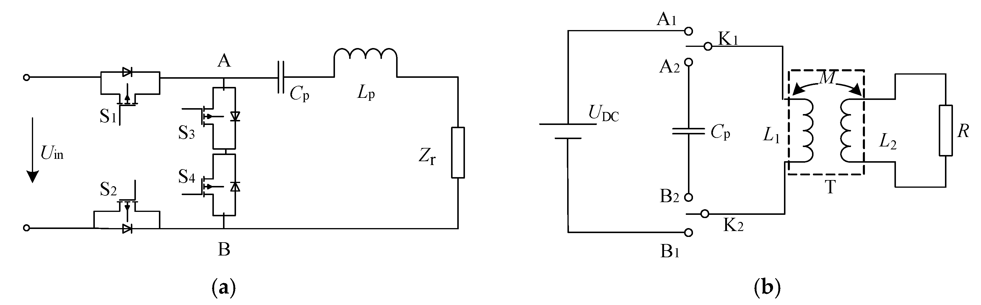
Figure 2.
Circuit models in the energy injection stage: (a) simplified circuit model; (b) equivalent circuit model.
Figure 2.
Circuit models in the energy injection stage: (a) simplified circuit model; (b) equivalent circuit model.

Figure 3.
Circuit models in the self-tuning stage: (a) T model; (b) simplified model.
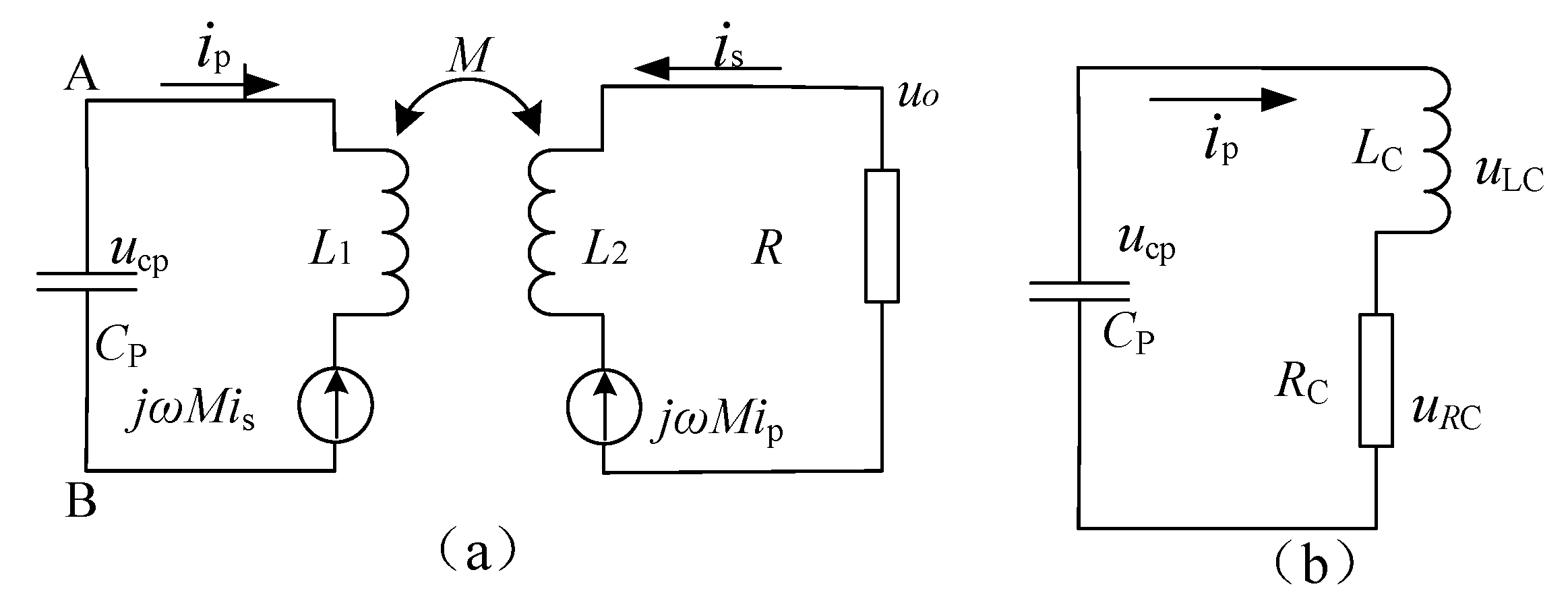
Figure 4.
Structure of the TSEIST power converter.
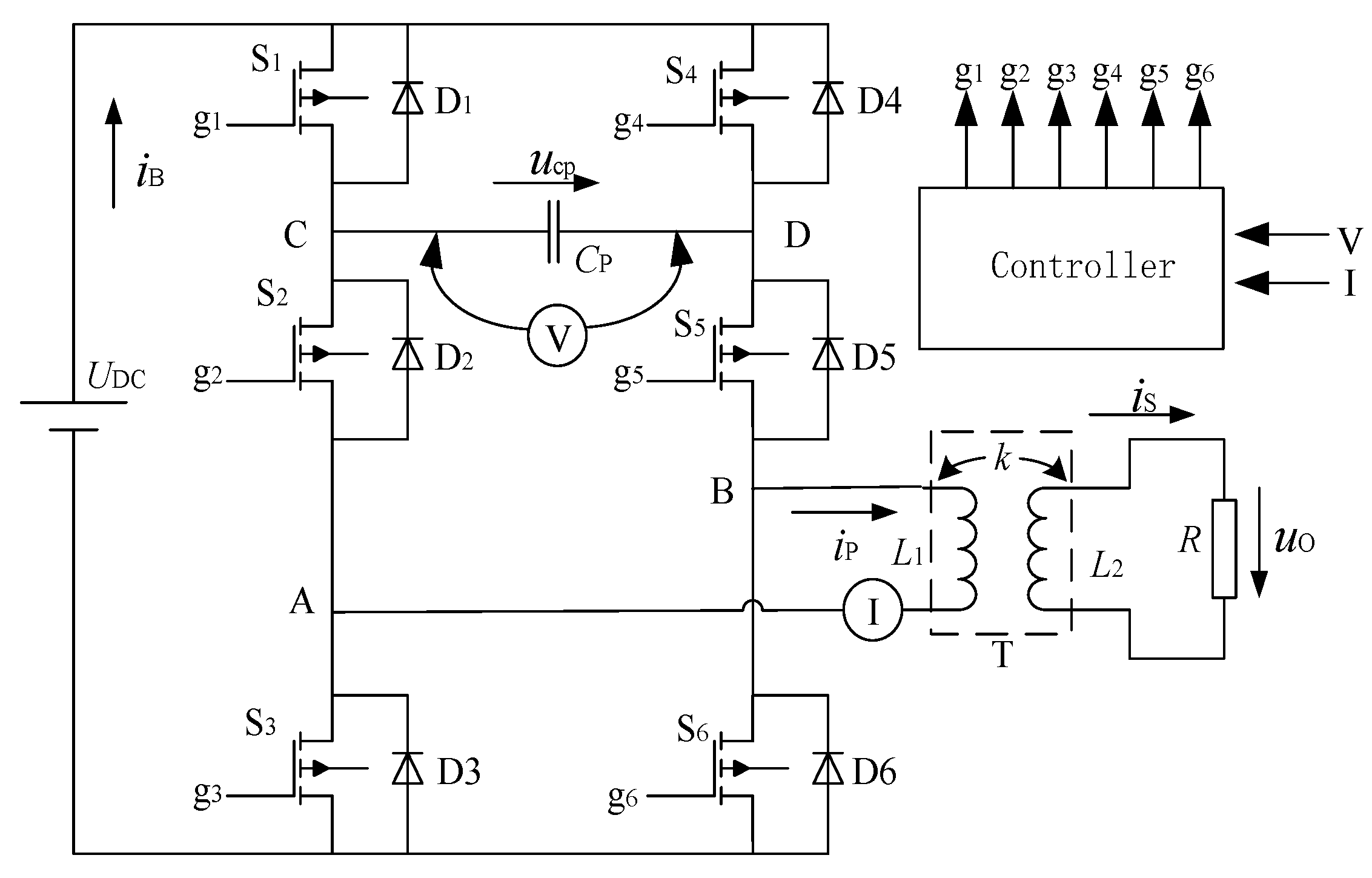
Figure 5.
State transitions of the TSEIST power converter.

Figure 6.
The waveforms of the bus current, primary current and tank capacitance voltage of the TSEIST converter.
Figure 6.
The waveforms of the bus current, primary current and tank capacitance voltage of the TSEIST converter.
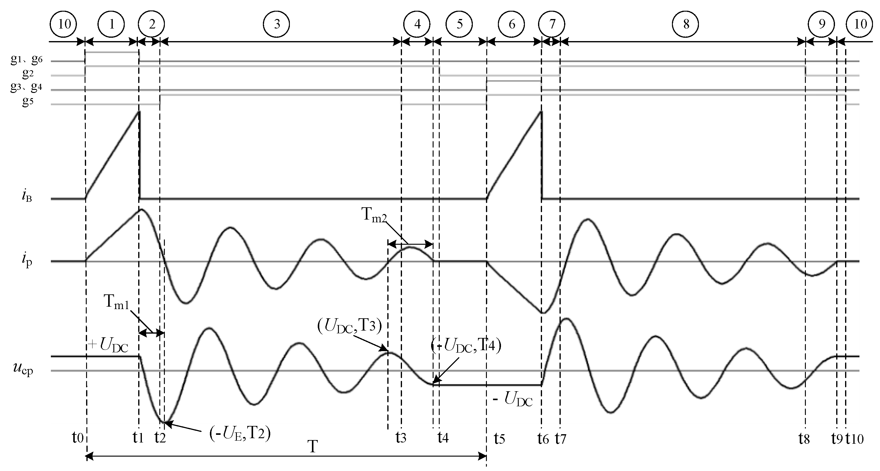
Figure 7.
The waveform of the voltage of the tank capacitor.
Figure 8.
Block diagram of the control logic.
Figure 9.
Structure of the coil pads.
Figure 10.
Coupling coefficient versus air gap.

Figure 11.
The prototype of the TSEIST power converter system.

Figure 12.
Results of bus current, primary coil current, and capacitor voltage (a) Simulation results (b) Experimental results (bus current in blue, primary coil current in purple, and capacitor voltage in red line).
Figure 12.
Results of bus current, primary coil current, and capacitor voltage (a) Simulation results (b) Experimental results (bus current in blue, primary coil current in purple, and capacitor voltage in red line).

Figure 13.
The output power versus energy injecting time τ1 at k = 0.5.
Figure 14.
The resonant frequency versus coupling coefficient k.
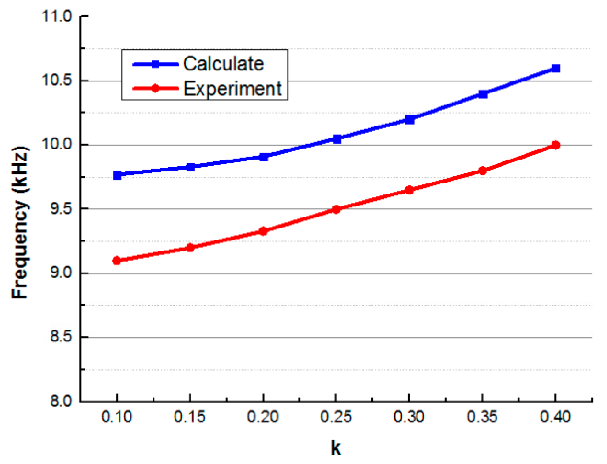
Figure 15.
Operating waves of switches (a) S1, (b) S2, and (c) S3 in the experiments.


Table 1.
State duration time.
| State Duration Time | Calculation Method |
|---|---|
| Δt0 | Δt0 = t5 − t4 = τ3 |
| Δt1 | Δt1 = t1 − t0 = τ1 |
| Δt2 | Δt2 = t2 − t1, 0 < Δt2 < Tm1 |
| Δt3 | Δt3 = t3 − t2, determined by Dp, Dr. |
| Δt4 | Δt4 = t4 − t3, 0 < Δt4 < Tm2 |
Table 2.
Parameters of the pads.
| D1 | D2 | D3 | D4 | D5 | D6 |
| 460 mm | 370 mm | 440 mm | 350 mm | 160 mm | 80 mm |
| H1 | H2 | H3 | H4 | W1 | W2 |
| 5 mm | 10 mm | 5 mm | 3 mm | 20 mm | 150 mm |
Table 3.
Main parameters of the power converter.
| Parameter/Part | Value |
|---|---|
| UDC | 300 V |
| Cp | 0.44 uF |
| L1, L2 | 640 uH |
| R | 50 Ω |
| S1–S6 | IXFN56N90 |
Table 4.
Output power and efficiencies for different coupling coefficients.
| k | 0.5 | 0.4 | 0.25 | 0.15 | 0.1 |
|---|---|---|---|---|---|
| Pin (W) | 350 | 350 | 350 | 350 | 350 |
| Pop (W) | 342 | 341.6 | 340.6 | 338.8 | 335.7 |
| Pos (W) | 327.6 | 326.6 | 324.5 | 314.3 | 303.5 |
| ηp (%) | 97.7 | 97.6 | 97.3 | 96.8 | 95.9 |
| ηs (%) | 93.6 | 93.3 | 92.7 | 89.8 | 86.7 |
© 2019 by the authors. Licensee MDPI, Basel, Switzerland. This article is an open access article distributed under the terms and conditions of the Creative Commons Attribution (CC BY) license (http://creativecommons.org/licenses/by/4.0/).
Share and Cite
MDPI and ACS Style
Chen, L.; Hong, J.; Guan, M.; Wu, W.; Chen, W. A Power Converter Decoupled from the Resonant Network for Wireless Inductive Coupling Power Transfer. Energies 2019, 12, 1192. https://doi.org/10.3390/en12071192
AMA Style
Chen L, Hong J, Guan M, Wu W, Chen W. A Power Converter Decoupled from the Resonant Network for Wireless Inductive Coupling Power Transfer. Energies. 2019; 12(7):1192. https://doi.org/10.3390/en12071192
Chicago/Turabian StyleChen, Lin, Jianfeng Hong, Mingjie Guan, Wei Wu, and Wenxiang Chen. 2019. "A Power Converter Decoupled from the Resonant Network for Wireless Inductive Coupling Power Transfer" Energies 12, no. 7: 1192. https://doi.org/10.3390/en12071192
Note that from the first issue of 2016, this journal uses article numbers instead of page numbers. See further details here.