Two-Terminal Algorithm Analysis for Unsymmetrical Fault Location on 110 kV Lines


Department of Electrical Power Engineering, Brno University of Technology, Technicka 12, 61600 Brno, Czech Republic
*
Author to whom correspondence should be addressed.
Energies 2019, 12(7), 1193; https://doi.org/10.3390/en12071193
Submission received: 5 March 2019
/
Revised: 24 March 2019
/
Accepted: 25 March 2019
/
Published: 27 March 2019
(This article belongs to the Special Issue Fault Diagnosis on MV and HV Transmission Lines)
Abstract
:This work analyses a two-terminal algorithm designed to locate unsymmetrical faults on 110 kV power transmission lines. The algorithm processes synchronized voltage and current data obtained from both ends of the protected transmission line and calculates the distance of the fault. It is based on decomposing the equivalent circuit into the positive-, negative- and zero-sequence components and finding the point where the output voltages of the right and the left side of the transmission line are equal. Compared to the conventional distance relay locator, the accuracy of this method is higher and less influenced by the fault resistance, the parallel-operated line effect and line asymmetry, as discussed in this work. It is, however, very sensitive to the synchronization accuracy. The mathematical model of the power system was created in the PSCAD (Power Systems Computer Aided Design) environment and the computational algorithm was implemented in Mathematica software.
1. Introduction
To locate a fault during single-phase faults in a 110 kV line, a fault locator, which is one of the functions of distance protection, is currently used. The basic parameters of a protected line are set in the relay and used to compute the fault distance and usually to initiate the locator function as well. Basically, after the pick up or the trip of the distance protection, a short-circuit loop is determined and the currents and voltages measured in this loop are used for the short-circuit loop reactance and resistance calculation. After that, a fault loop and its impedance through the measured phase currents and voltages are determined. If a ground fault location is calculated, it is necessary to take account of values of the residual compensation factors RE/R1, XE/X1 as well. The computational algorithm used for the fault impedance determination is based on the solution of the short-circuit loop using the value of the voltage measured at the protection connection point, the current in the forward direction (to the fault) and the current in the backward direction (back to the point of measurement). In the case of a single-phase fault in phase i (i = 1, 2, 3) it will be:
The fault distance is evaluated from the reactance to the fault , which is the imaginary component of the fault impedance . Thus, the correct evaluation of the single-phase fault distance is always strongly dependent on the reactance per kilometer and residual compensation factor of the protected line set in the distance relay.
Since most of the 110 kV lines are not fully transposed, fault locator errors are often caused by unequal impedance values of the phase-ground loops and mutual impedances of these loops. Another error can be caused by non-homogeneity of the transmission line. Non-homogeneity means that the line parameters are not constant for the whole line length but vary in individual sections. Typical examples are changes in cross-section or different ground wire conductivity. Negative effect of the fault resistance on fault location is described in [1,2]. In systems with parallel-operated lines, the accuracy of the fault location is also greatly influenced by mutual impedances. In general, the ground wire conductivity and the short-circuit contribution of the parallel line power supply will have the major influence on the locator error rate.
Many researchers have focused their attention on possible error elimination. The proposed algorithms differ depending on the input data they have available and the method of calculation. The methods can be divided into three main groups:
- Travelling wave-based methods,
- Artificial intelligence-based methods,
- Impedance-based methods.
1.1. Travelling Wave- and Artificial Intelligence-Based Methods
Travelling wave-based computational methods are usually based on the correlation between the forward and backward waves that travel alongside the transmission line. When a fault occurs, the waves travel from the point of the fault to both ends of the transmission line. The fault is then identified using the transient-state analysis. Some studies [3,4] suggest creating a database of various fault scenarios to make the transient analysis easier.
These methods can work with one- or multiple-terminal data. The accuracy of these algorithms is mainly dependent on the data sampling rate. For the fault detection, the wavelet transform proves to be very reliable.
Intelligent techniques help to improve efficiency of the fault detection and classification. The advantage of using neural network is its ability to recognize a pattern and categorize the data. According to [5], the most used techniques based on the artificial intelligence are:
- Expert System Techniques,
- Artificial Neural Networks,
- Fuzzy Logic Systems.
Recently, a use of time-time (TT) transform in signal processing has been discussed [6]. Reference [7] proposes to apply TT-transform to series-compensated lines, which proved to be efficient even when processing a signal influenced by high noise. In [8], the TT-transform and a fault classification based on support vector machine (SVM) is used to locate fault on a hybrid line. Although this technique processes transient voltage signal obtained from only one end, the fault was identified and located with a high accuracy.
1.2. Impedance-Based Methods
The basic principle of the impedance-based algorithms for the fault location calculation is simple. The protection relay uses positive and zero sequence impedances and measured voltages and currents to determine the distance to the fault by calculating the impedance, as described by Equation (1). These methods are simple and commonly used and their accuracy can be significantly improved if data from multiple terminals is acquired.
Algorithms that use only local measurement data are called single-ended (or one-terminal) algorithms. These methods are often implemented, e.g., in microprocessor-based protective relays [9,10]. Their advantages are simplicity due to their lack of communication requirements. However, the accuracy of these methods is greatly influenced by fault resistance, load flow and source impedances. In [11], a single-ended technique, which is based on using the current and voltage measurements at local terminal and an estimated short-circuit capacity of the remote system, is proposed. Although this method is not unaffected by the problems mentioned above, the errors were within acceptable limits.
Two-terminal algorithms work with the measurements from both ends of the transmission line. These algorithms can be further divided into methods using synchronized or unsynchronized measurements. It is also possible to process data from multiple terminals to improve the accuracy of the calculation.
Using the synchronized two-terminal voltage and current phasors, the calculation of the fault location is significantly improved [1]. The data collected from digital recorders is evaluated in a central computer using specialized software. With the telecommunications development, the synchronization and fast and reliable measured phasor data exchange are becoming easier and therefore it is possible to implement these algorithms directly into the protection. The advantages of these methods are:
- Elimination of fault location errors caused by inaccuracies in residual compensation factors determination,
- Suppression of an error caused by the fault resistance,
- Reduction of the effects of mutual coupling and line asymmetry.
The impedance-based methods are currently the most widely used methods of fault location and with the development and installation of the phasor measurement units (PMUs) or digital relays with global positioning systems, the techniques based on the fundamental power frequency components can be improved. The biggest advantage of these techniques, proposed e.g., in [12,13,14], is that the error caused by variations in the source and fault impedances is eliminated. Extensive placing of the PMUs is, however, very limited by the high installation costs and therefore, some works focus on developing an optimal PMU placement strategy [12]. Moreover, the developed techniques are often influenced by other factors, such as need of high data sampling rate [14].
Reference [13] proposes a method that utilizes synchronized voltage and current data derived at both ends of the transmission line and expresses the voltage across the fault in terms of the measured data. This work is based on similar principle and it will be discussed later in this text. Compared to [13], however, the exact evaluation of the fault distance is not performed. Instead, the accuracy of the analyzed algorithm is improved by using not only positive-, but negative-sequence components as well. Then, the least square method is applied to find the point of the fault.
Some papers [15,16,17] try to remove the need of obtaining synchronized data. Reference [15] suggests modifying the technique introduced in [13] by considering only the magnitudes of the voltage at the fault point. This assumption allows to use unsynchronized phasors of measured voltages and currents and remove the error caused by the unsynchronized data. Methods described in [16,17] are based on a simple assumption that a fault impedance is purely resistive. Finding a solution to this condition is then used to find the synchronization angle.
Although these algorithms enable to use the unsynchronized measurements, which is a big improvement, the main aim of this work is to find a usable method for the fault location on 110 kV lines in the Czech Republic, which are short and often parallel-operated. Methods proposed in [15,16,17] do not deal with the effect of the parallel line. In this work, the effect of mutual coupling is fully considered.
2. Description of the Analyzed Algorithm
Firstly, a method using the one-terminal approach will be described to outline a basic principle of the proposed impedance-based algorithm and the errors that can occur. The parallel-operated line effect is described here as well. Later in this section, an analyzed two-terminal algorithm will be discussed.
2.1. Basic Description of the One-Terminal Algorithm
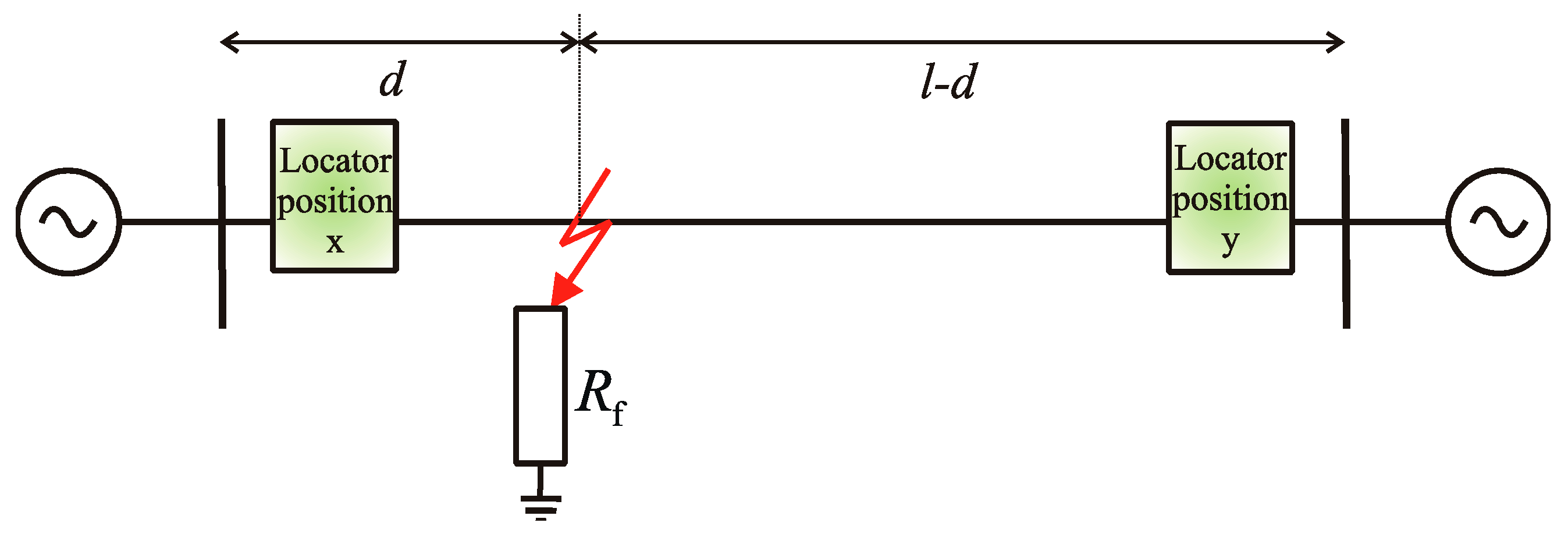
Figure 1 displays a situation when a single-phase fault with a fault resistance Rf occurs in a transmission line. The fault is located in the distance d measured from the locator at the x-point, the total line length is l. Using this example, an idea of one-terminal algorithm errors can be given.
An equivalent circuit is formed by the interconnection of impedance sequence component circuits and the fault resistance—see Figure 2. The indexes for the positive, negative and zero-sequence components are 1, 2 and 0, respectively. If the Kirchhoff’s circuit laws are applied in individual loops of the equivalent circuit, an evaluation of the fault distance d using the current and voltage ratio used by the locator placed at the x-point can be done:
If (where and are line impedances per unit length of a zero- and positive-sequence component, respectively, and is a residual compensation factor) is assumed, then:
where the voltage at the fault point can be written as:
Applying these equations, the impedance measured by the locator at the x-point is:
and similarly, for the locator placed at the y-point:
If the line parameters and , fault resistance Rf and the earth currents and acquired from both ends are known, the Equations (6) and (7) can be used to precisely calculate the fault distance. If these values are not obtained, the locator algorithm correction method will always be just an estimation and therefore potentially able to actually increase the locator error. Even more complicated situation occurs for the parallel-operated lines, when the equivalent circuit contains also the parallel-line sequence impedances—in the Figure 2 drawn in red.
From the circuit diagram it is clear that the positive and the negative sequence components of the impedance measured by the locator remain the same, but the zero sequence does not. This is caused by the common path of the earth current for both transmission lines formed by the ground and the ground wire. The mutual coupling is symbolized in the zero-sequence component by four additional induced voltage sources. Two of them are part of the zero-sequence component of the faulted section. These voltages are induced by the zero-sequence current of the parallel line:
The remaining two voltage sources are located in the zero-sequence component of the healthy line and are induced by the zero-sequence current of the faulty line:
Voltages can be substituted for product of currents that induce these voltages and mutual zero sequence impedance according to Equations (8)–(11). Then, the equivalent circuit of the zero-sequence impedance can be modified, as shown in Figure 3.
The locator placed at the x-point calculates the impedance as
For the locator placed at the y-point can be written as:
It is obvious that due to the number of quantities that influence the impedance calculation, it is much more effective to use two-terminal algorithms.
2.2. Two-Terminal Algorithm
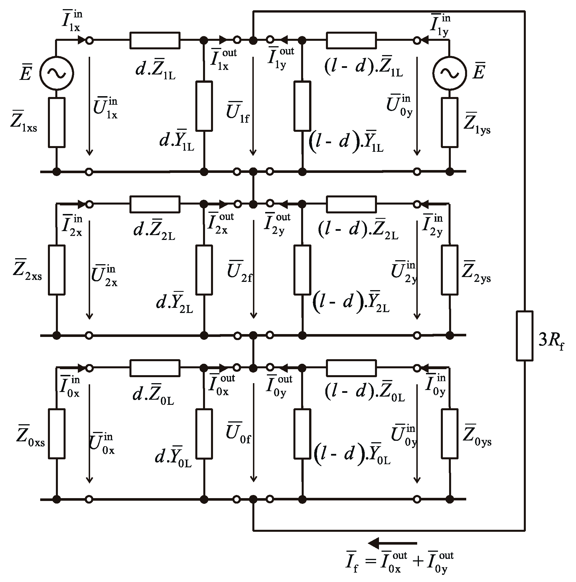
The equivalent circuit used for two-terminal algorithms is displayed in Figure 4. The transmission line between the source and the fault point is substituted by the distributed parameter line model with series impedances and shunt admittances. The complete equivalent circuit consists of individual sequence component circuits connected to the fault resistance Rf.
To calculate the fault location, individual sequence component voltages at the fault point (where i = 1, 2, 0) are determined. These voltages represent the output voltages of the respective transmission line model and can be calculated using the input values of currents and voltages at the x-point:
or using the input values of currents and voltages at the y-point:
where is the propagation constant and is the characteristic impedance of the protected transmission line (i = 1, 2, 0 for the positive-, negative- and zero-sequence component of the line impedance per unit length and the line admittance per unit length ).
If , then the fault location d can be determined. For this purpose, the positive-sequence component can be used because its parameters and are known and their calculation is not influenced by the soil resistivity.
If the right sides of the Equations (15) and (16) are equal, then it is possible to use only the equations for the positive-sequence voltage at the fault point
Assuming and , to increase the calculation reliability, the negative-sequence voltage is used as well
For each equation, a deviation from zero for various values of d can be determined
After obtaining the deviations for positive- and negative-sequence component and applying the least square method, a simple function F is created. This function reaches its minimum in the distance d, which corresponds to the fault point:
The output of this algorithm is the value of distance d with the minimal F(d) value.
2.3. Synchronization
To correctly calculate the distance of the fault d using this algorithm, it is necessary to measure the input currents and voltages at x- and y-points synchronously. This, however, is mostly impossible in current 110 kV distribution networks. The distance protection locators do not use mutual time synchronization; therefore, the data records must be additionally synchronized before performing the calculations. This can be done with use of the transient data records in the time domain, e.g., capturing the moment of the transient inception (a sufficient data sampling rate required). Another method is based on the phasor correction by estimating the input quantities mutual phase shift. Using this estimated phase shift value, the corresponding quantities are shifted by angle -synchronization operator. If is the synchronizing quantity, then:
- Phasor correction at the x-point: , ,
- Phasor correction at the y-point: , ,
where are the angles of the unsynchronously recorded phasors and is the synchronization operator determined by the phase shift of the currents and .
Considering the 110 kV distribution networks operation, the phase shift between the input currents can be determined using the short-circuit impedances and representing the protected line load, as shown in a simplified diagram in Figure 5. According to [1], to estimate the synchronization operator , the input current and voltage data captured during the normal operation or during the fault (or their combination) can be used. The same principle of the synchronization in [13] is used.
Another method is, as mentioned above, based on transient observation. To analyze the frequency components of the signal, the Fourier transform is commonly used. The problem with using Fourier transform is that it is not capable to determine when the particular frequency changes. To acquire information about both time and frequency, a short-time Fourier transform, which uses a sliding window, can be applied. This technique, however, limits the frequency resolution. Better solution is to use the wavelet transform [18]. The wavelet transform decomposes the signal into functions located both in Fourier and the real-time space. It is basically an infinite set of various transforms.
The problem with records synchronization using the transient study is the unequal time that the transient needs to get from the fault point to the point of measurement. The transient arrives sooner at the closer terminal, so capturing the moment of the transient inception at both terminals and subsequent comparison can be quite inaccurate. Future research will be focused on this topic.
The synchronization method should be chosen based on the data availability. However, the preferable one is the transient analysis method. If the required data are not available, the synchronization operator needs to be calculated.
3. Analysis of the Two-Terminal Algorithm Testing
3.1. Mathematical Model of a 110 kV Line
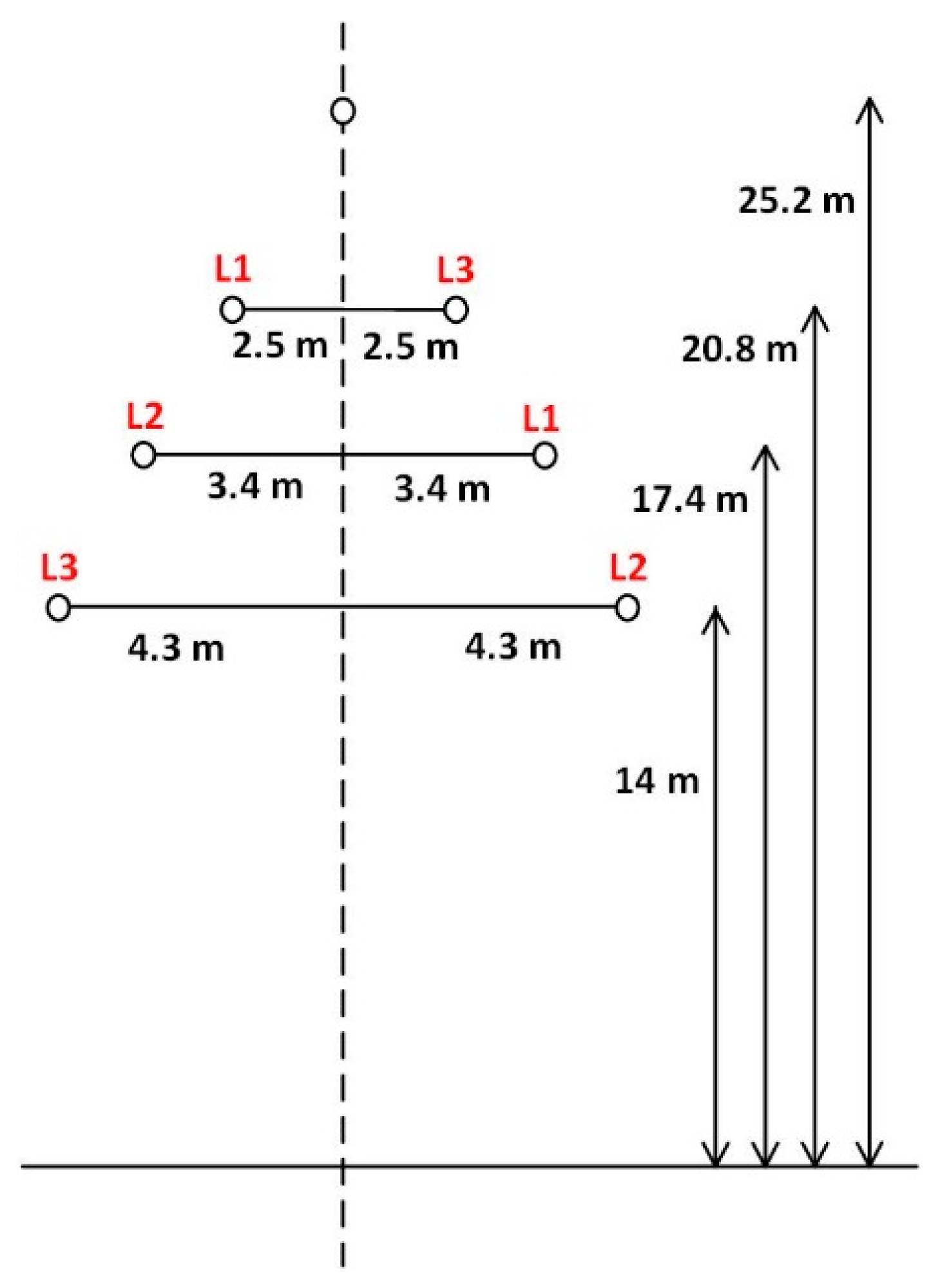
The presented two-terminal algorithm was implemented in the Mathematica software (version 11.1.1.0, Wolfram Research, Champaign, IL, USA) to process the voltages and currents measured at both ends of the 110 kV line modelled in PSCAD software (version 4.6.0.0, Manitoba HVDC Research Centre, Winnipeg, MB, Canada). The voltage and current data are obtained synchronously, which means that quantities mutual time shift is zero. The created model consists of two non-transposed parallel-operated 110 kV lines with six conductors and one ground wire, as in Figure 6. One side of the tower carries the conductors of the first line, the other side carries the second line. The mathematical model of this line is built according to the real distribution parallel-operated 110 kV line.
The transmission line is modelled using the frequency dependent line model. The soil resistivity is 50 Ωm, the length of the line is 27.88 km. There are six 240 AlFe4 conductors and a combined ground wire with 48 fibers (0.2 Ω DC resistance and 18 mm diameter). Line parameters were derived from series impedance and shunt admittance matrixes in PSCAD line constant program output file. The results are listed in Table 1.
Using the created PSCAD model, it is also possible to calculate the fault distance. To do this, the Equation (1) is used similarly to the common fault locator. The computational algorithm is built with logical blocks and functions implemented in the PSCAD library. It utilizes obtained current and voltage data processed using the Fast Fourier Transform. The output of this calculation can be compared to the output of the proposed algorithm.
The simulation data are stored in a Comtrade file format. The PSCAD software contains a component called RTP/COMTRADE Recorder, which is able to record the simulated data a save them as Comtrade. Therefore, the data can be further viewed in a software that uses this format.
3.2. Impact of the Fault Resistance
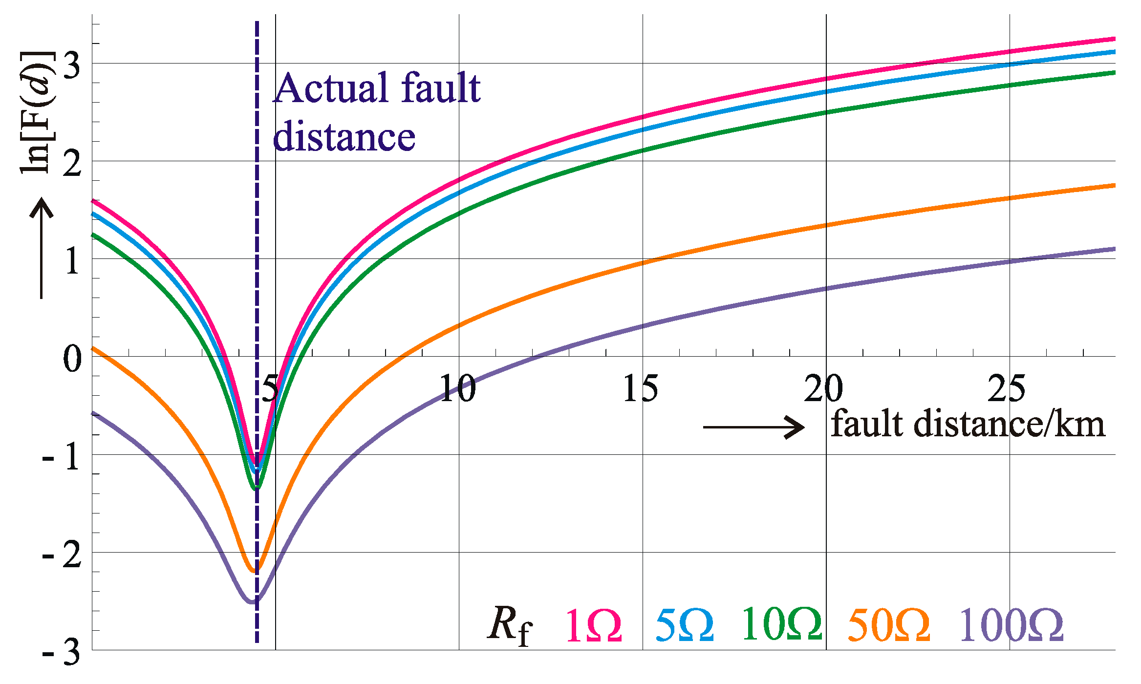
Several tests were performed to assess the impact of the fault resistance value on the proposed algorithm. The fault occurred in the L1 phase in the distance of 4.49 km from the terminal at the x-point. The fault resistance was changed up to 100 Ω, which appears very rarely in the 110 kV network and even a fault with such high resistance was successfully localized, as seen in Figure 7, where the minimum of the function denotes the calculated fault location.
Table 2 summarizes the test results. The errors of the two-terminal algorithm are compared to the errors given by the calculation that performs the created PSCAD computational algorithm used by a conventional distance relay locator. The fault distance from the x-point terminal was 4.49 km, the distance from the y-point terminal was 23.39 km. Table 2 shows the errors of the fault location both in absolute (m) and relative (%) values. It is obvious that a higher fault resistance means a higher error, especially when using the one-terminal approach of the distance relay locator.
Calculated errors are expressed with respect to the fault distance measured from the terminal, where the evaluated data is acquired. The absolute error is calculated as:
and the relative error as:
Absolute error = (Estimated distance from the terminal) − (Actual distance from the terminal)
3.3. Impact of the Parallel Line
Considering the one-terminal approach, the parallel-operated line effect will be more significant for more remote faults. Figure 8 shows the results of the proposed algorithm for the faults in the distances of 2.5, 11.2, 16.8 and 25 km from the terminal at the x-point. From the figure it is obvious that algorithm results fully respond to actual fault distances. Unlike the one-terminal approach of the conventional distance relay locator, the accuracy of the proposed algorithm is not influenced by the fault distance and the associated parallel line mutual coupling, as seen in Figure 9.
3.4. Impact of the Line Parameters (Line Asymmetry)
The impact of the series impedance asymmetry is evaluated by applying the algorithm to the faults in different phases of the non-transposed transmission line. It means that while the phase-to-ground loop parameters are not the same for every phase, the algorithm still uses the same positive-, negative- and zero-sequence component values of the ideally transposed lines.
This impact can be seen in Figure 10 and Figure 11. The test was carried out for every phase and for various fault resistances. The fault occurred in the distance of 4.49 km from the terminal at the x-point. It can be concluded that for smaller fault resistances the proposed two-terminal algorithm evaluates the fault distance with a satisfactory accuracy for every phase. However, higher fault resistance significantly decreases the accuracy of the algorithm. This can be seen in Figure 11, which depicts the errors of the calculation related to the closer terminal (x-point).
3.5. Impact of the Synchronization Accuracy
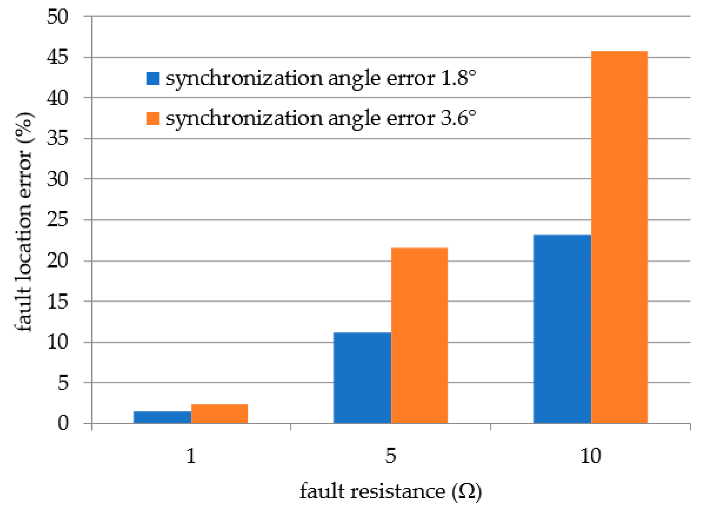
The PSCAD mathematical model uses unified time for all the records. Therefore, all data is perfectly synchronized. To evaluate an impact of the synchronization accuracy, angles of voltages and currents measured at one side of the transmission line were shifted by an angle δ. Figure 12 shows the results obtained from processing the faults in the L1 phase with different fault resistances. The results prove a significant algorithm sensitivity to the synchronization accuracy. For the faults with the bigger fault resistance, the influence of the synchronization error becomes even more obvious. A small angle error of 1.8° (which correspond to 0.1 ms time error) causes that the algorithm evaluates the fault location with a great inaccuracy. At this point, the algorithm becomes unusable. Figure 13 summarizes these results in a bar chart. It is obvious, that the algorithm sensitivity to the synchronization accuracy is the bigger, the bigger the fault resistance is.
4. Conclusions
Accurate fault location on transmission lines is still a very topical issue. In this article, an impedance-based single-phase fault location method is presented and analyzed. With some modifications discussed in the Introduction, this method is based on a technique presented in [13]. It uses a distributed parameter line model and synchronized two-terminal voltage and current data obtained from PSCAD simulations.
One of the goals of this work was to evaluate if this method could be applicable to the shorter 110 kV transmission lines common in Central Europe. The effect of the fault resistance, line asymmetry and parallel-operated line has been discussed. The analyzed algorithm was able to locate the faults for all the tested scenarios with sufficient accuracy. To achieve this, however, an accurate data synchronization is required. As discussed in this article, even a small synchronization angle error causes a major decrease of the algorithm accuracy. Future research will be dedicated to possible data synchronization methods.
Author Contributions
Conceptualization, J.O. and P.T.; Data curation, Z.B. and J.O.; Formal analysis, Z.B. and J.O.; Investigation, Z.B.; Methodology, Z.B., J.O. and D.T.; Project administration, P.T.; Resources, D.T.; Supervision, J.O.; Visualization, Z.B.; Writing—original draft, Z.B. and J.O.
Funding
This research was funded by the Ministry of Education, Youth and Sports of the Czech Republic under OP VVV Programme (project No. CZ.02.1.01/0.0/0.0/16_013/0001638 CVVOZE Power Laboratories—Modernization of Research Infrastructure).
Acknowledgments
Authors gratefully acknowledge the Centre for Research and Utilization of Renewable Energy (CVVOZE) where this research work was carried out.
Conflicts of Interest
The authors declare no conflict of interest.
References
- Ziegler, G. Numerical Distance Protection, 2nd ed.; Publicis Corporate Publishing: Erlangen, Germany, 2006; pp. 126–147. ISBN 3-89578-266-1. [Google Scholar]
- Makwana, H.; Bhavesh, V.; Bhavesh, B. Distance Relaying Algorithm for a Single Line-To-Ground Fault on Single Infeed Transmission Lines. In Energy Systems in Electrical Engineering; Springer: Singapore, 2016; pp. 17–40. [Google Scholar]
- Pinto Moreira de Souza, D.; da Silva Christo, E.; Rocha Almeida, A. Location of Faults in Power Transmission Lines Using the ARIMA Method. Energies 2017, 10, 1596. [Google Scholar] [CrossRef]
- Tang, J.R.; XiangGen, Y.; Zhe, Z.; ZhiQuin, H.; Lei, Y.; Wang, Y. Fault location in distribution networks using Prony analysis. In Proceedings of the 2011 International Conference on Advanced Power System Automation and Protection, Beijing, China, 12 April 2011; pp. 54–59. [Google Scholar]
- Wadhe, N.S.; Juware, R.A.; Khalsa, N.N. Determining fault location on Transmission Line using Distance Relay. Int. J. Innov. Emerg. Res. Eng. 2016, 3, 625–630. [Google Scholar]
- Pinnegar, C.R.; Mansinha, L. A method of time–time analysis: The TT-transform. Digit. Signal Process. 2003, 13, 588–603. [Google Scholar] [CrossRef]
- Gashteroodkhani, O.A.; Vahidi, B.; Zaboli, A. Time-time matrix z-score vector-based fault analysis method for series-compensated transmission lines. Turk. J. Electr. Eng. Comput. Sci. 2017, 25, 2647–2659. [Google Scholar] [CrossRef]
- Gashteroodkhani, O.A.; Majidi, M.; Etezadi-Amoli, M.; Nematollahi, A.F.; Vahidi, B. A hybrid SVM-TT transform-based method for fault location in hybridtransmission lines with underground cables. Electr. Power Syst. Res. 2019, 170, 205–214. [Google Scholar] [CrossRef]
- Takagi, T.; Yamakoshi, Y.; Yamaura, M. Development of a New Type Fault Locator Using the One-Terminal Voltage and Current Data. IEEE Trans. Power Appar. Syst. 1982, PAS-101, 2892–2898. [Google Scholar] [CrossRef]
- Eriksson, L.; Saha, M.M.; Rockefeller, G.D. An Accurate Fault Locator with Compensation for Apparent Reactance in the Fault Resistance Resulting from Remote-end Infeed. IEEE Trans. Power Appar. Syst. 1985, PAS-104, 424–436. [Google Scholar] [CrossRef]
- Lima, D.A.C.; Ferraz, R.G.; Filomena, A.D.; Bretas, A.S. Electrical power systems fault location with one-terminal data using estimated remote source impedance. In Proceedings of the 2013 IEEE Power & Energy Society General Meeting, Vancouver, BC, Canada, 21–25 July 2013; pp. 1–5. [Google Scholar]
- Lien, K.P.; Liu, C.W.; Yu, C.S.; Jiang, J.A. Transmission network fault location observability with minimal PMU placement. IEEE Trans. Power Deliv. 2006, 21, 1128–1136. [Google Scholar] [CrossRef]
- Johns, A.T.; Jamali, S. Accurate fault location technique for power transmission lines. IEE Proc. C Gener. Transm. Distrib. 1990, 137, 395–402. [Google Scholar] [CrossRef]
- Kezunovic, M.; Perunicic, B. Automated transmission line fault analysis using synchronized sampling at two ends. IEEE Trans. Power Syst. 1996, 11, 441–447. [Google Scholar] [CrossRef]
- Dalcastagne, A.L.; Filho, S.N.; Zurn, H.H.; Seara, R. An Iterative Two-Terminal Fault-Location Method Based on Unsynchronized Phasors. IEEE Trans. Power Deliv. 2008, 23, 2318–2329. [Google Scholar] [CrossRef]
- Yu, C.S. An Unsynchronized Measurements Correction Method for Two-Terminal Fault-Location Problems. IEEE Trans. Power Deliv. 2010, 25, 1325–1333. [Google Scholar] [CrossRef]
- Yu, C.S.; Chang, L.R.; Cho, J.R. New Fault Impedance Computations for Unsynchronized Two-Terminal Fault-Location Computations. IEEE Trans. Power Deliv. 2011, 26, 2879–2881. [Google Scholar] [CrossRef]
- Mehala, N.; Dahiya, R. A Comparative Study of FFT, STFT and Wavelet Techniques for Induction Machine Fault Diagnostic Analysis. In Proceedings of the 7th WSEAS International Conference on Computational Intelligence, Man-Machine Systems and Cybernetics, Cairo, Egypt, 29–31 December 2008; Zaharim, A., Mastorakis, N., Gonos, I., Eds.; World Scientific and Engineering Academy and Society (WSEAS): Stevens Point, WI, USA, 2008; pp. 203–208. [Google Scholar]
Figure 1.
A simplified faulty transmission line scheme.

Figure 2.
The equivalent circuit for parallel-operated transmission lines.
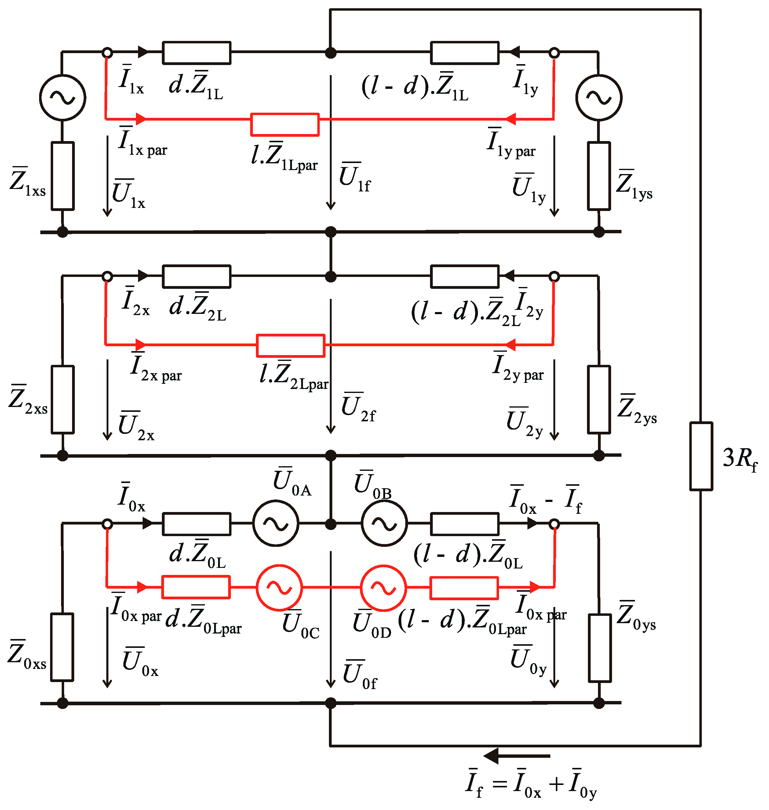
Figure 3.
A zero-sequence component equivalent circuit for parallel-operated transmission lines.
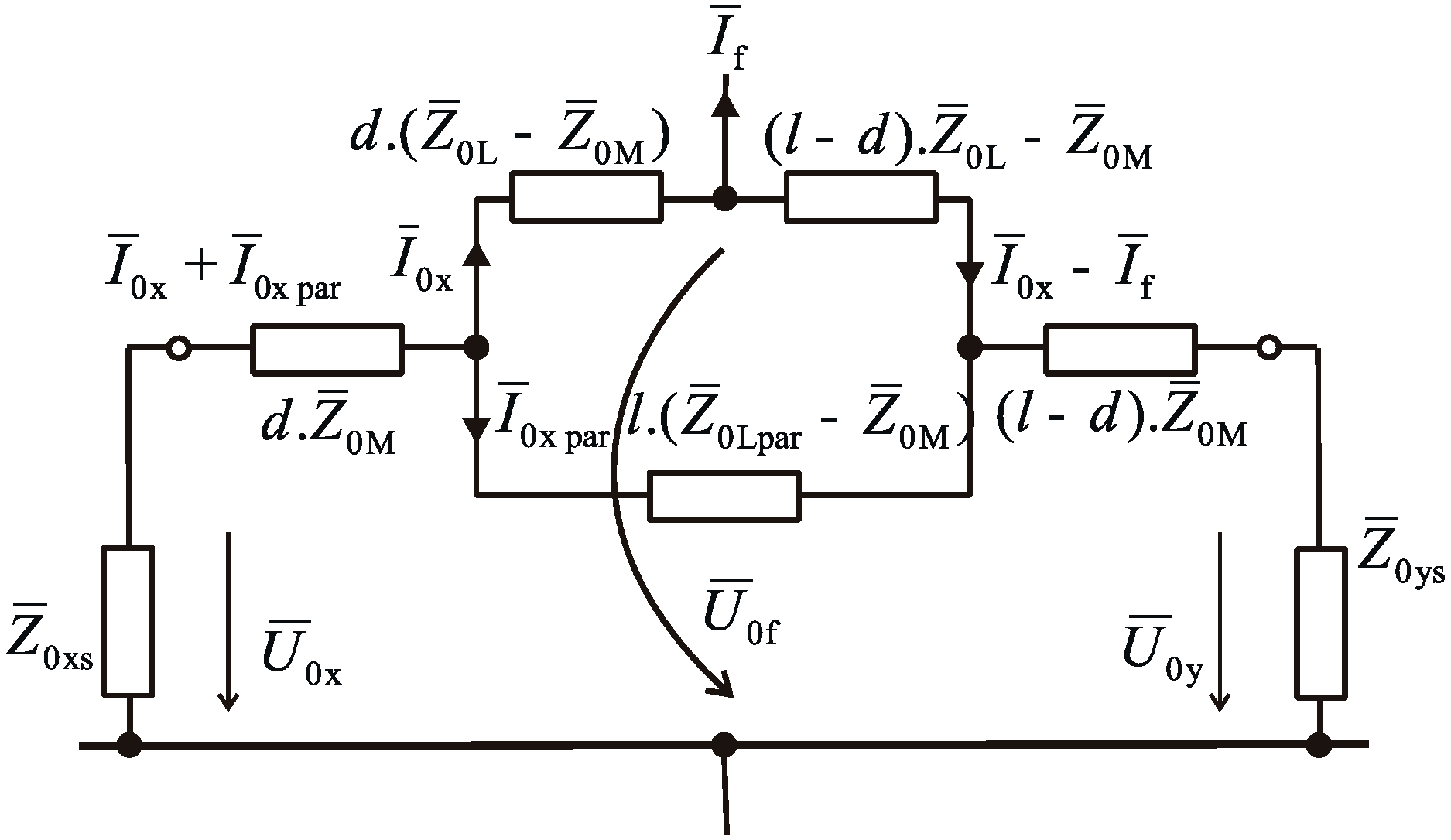
Figure 4.
An equivalent circuit for a single-phase fault.

Figure 5.
A simplified equivalent circuit for a single-phase fault.
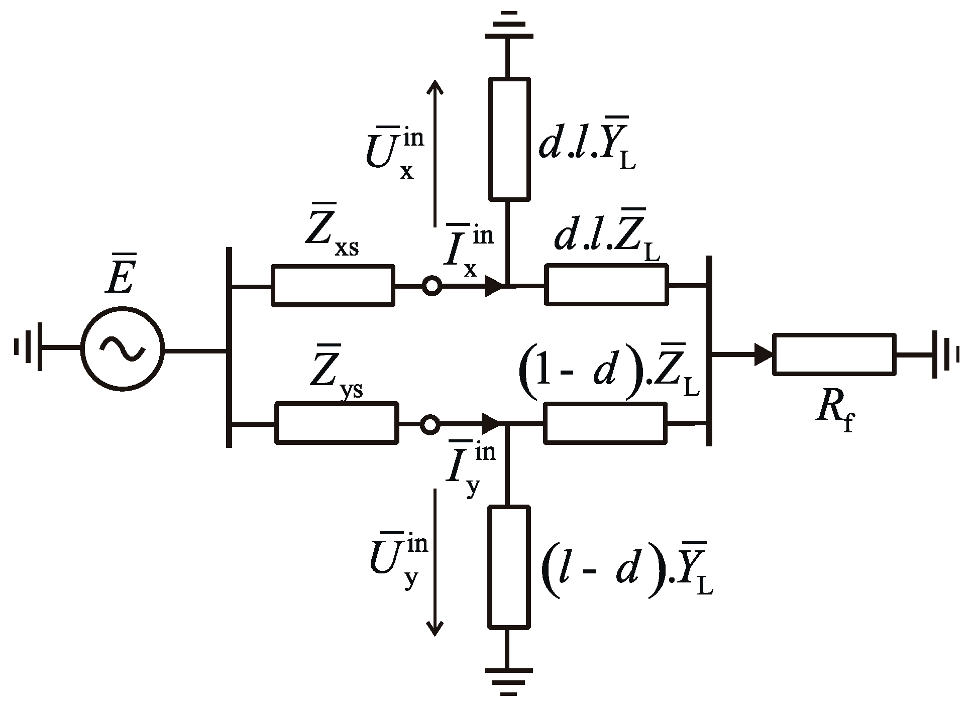
Figure 6.
Transmission line conductor arrangement.

Figure 7.
Fault resistance impact on two-terminal fault location (the actual fault distance 4.49 km).
Figure 7.
Fault resistance impact on two-terminal fault location (the actual fault distance 4.49 km).

Figure 8.
Results of the proposed algorithm for various fault distances.
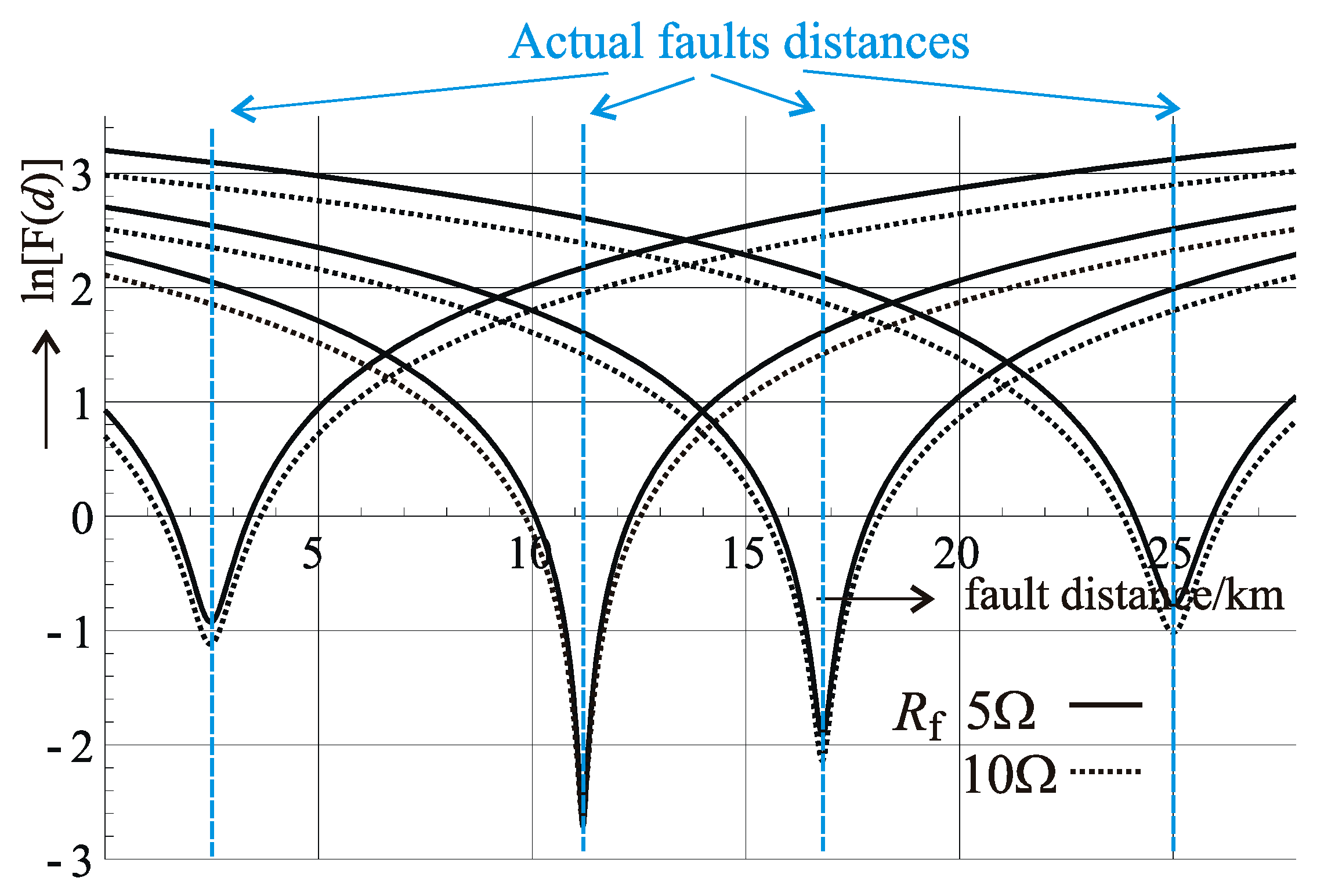
Figure 9.
The errors comparison between the proposed algorithm and the distance relay locator.
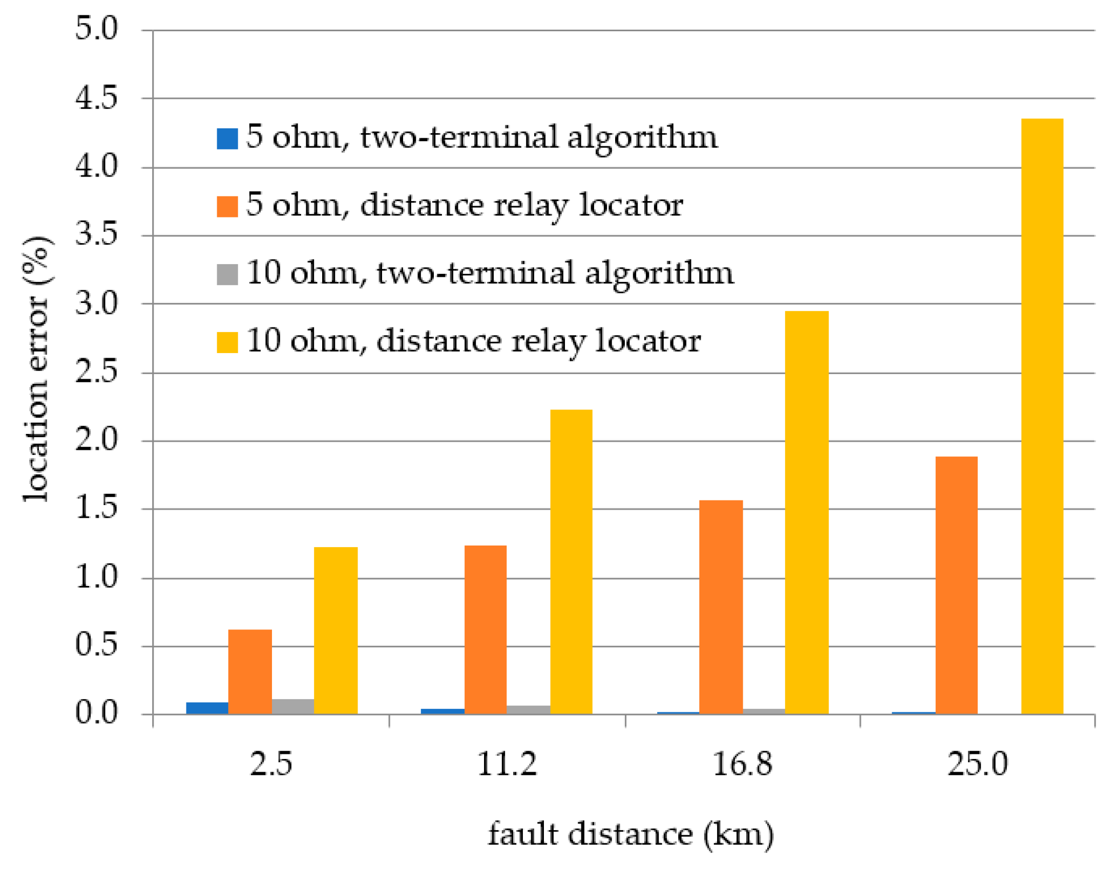
Figure 10.
The line asymmetry impact on the fault location calculation.
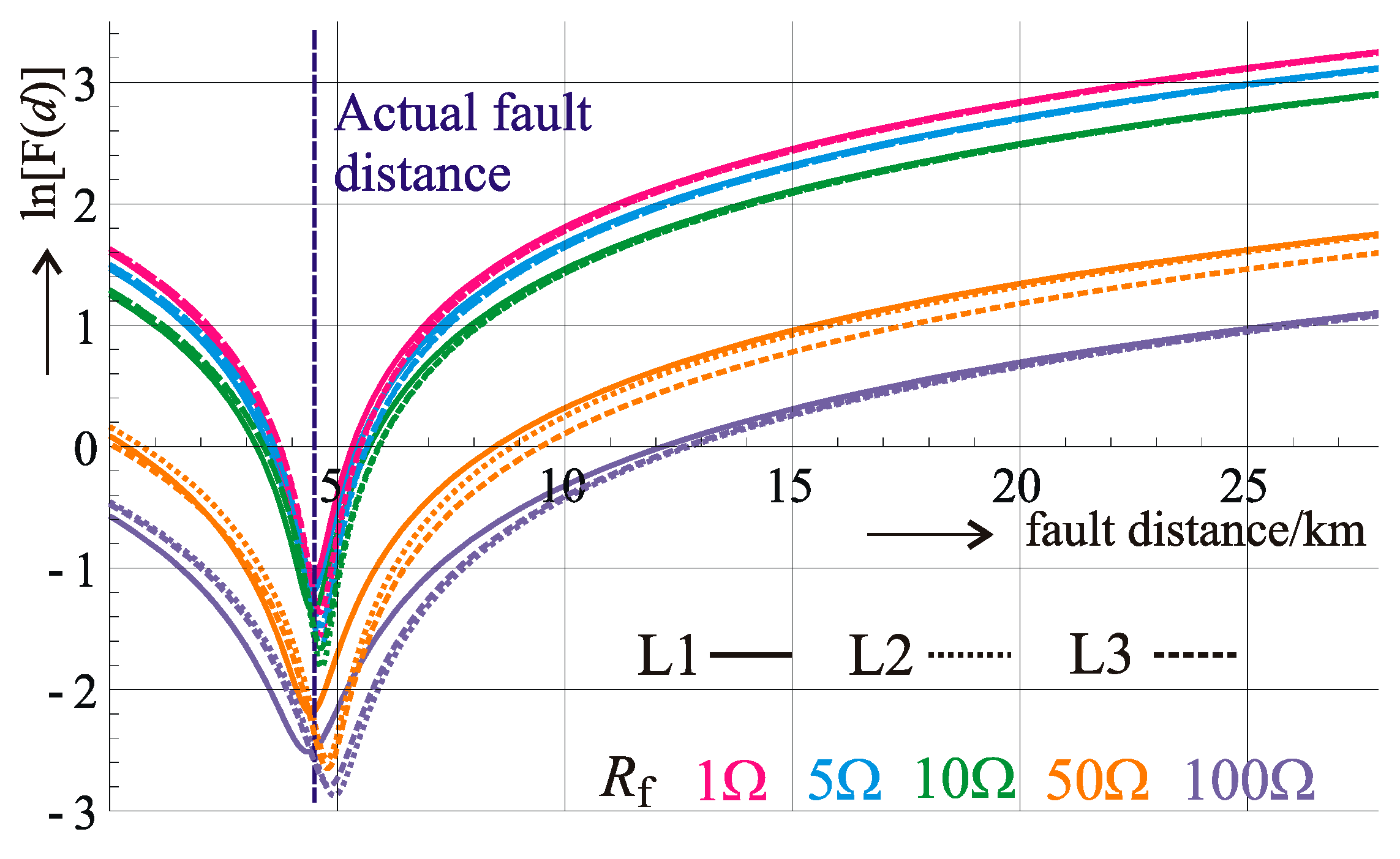
Figure 11.
The errors comparison for individual phases.
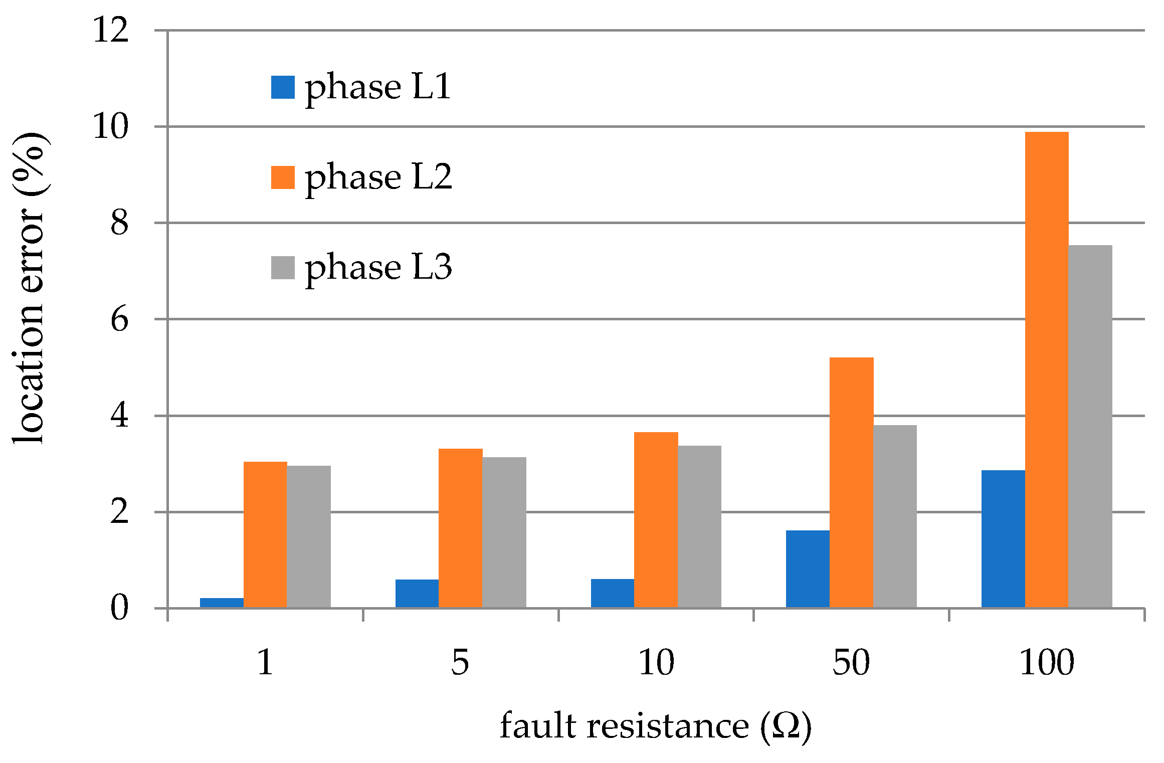
Figure 12.
Algorithm outputs comparison for various fault resistances and synchronization angles.
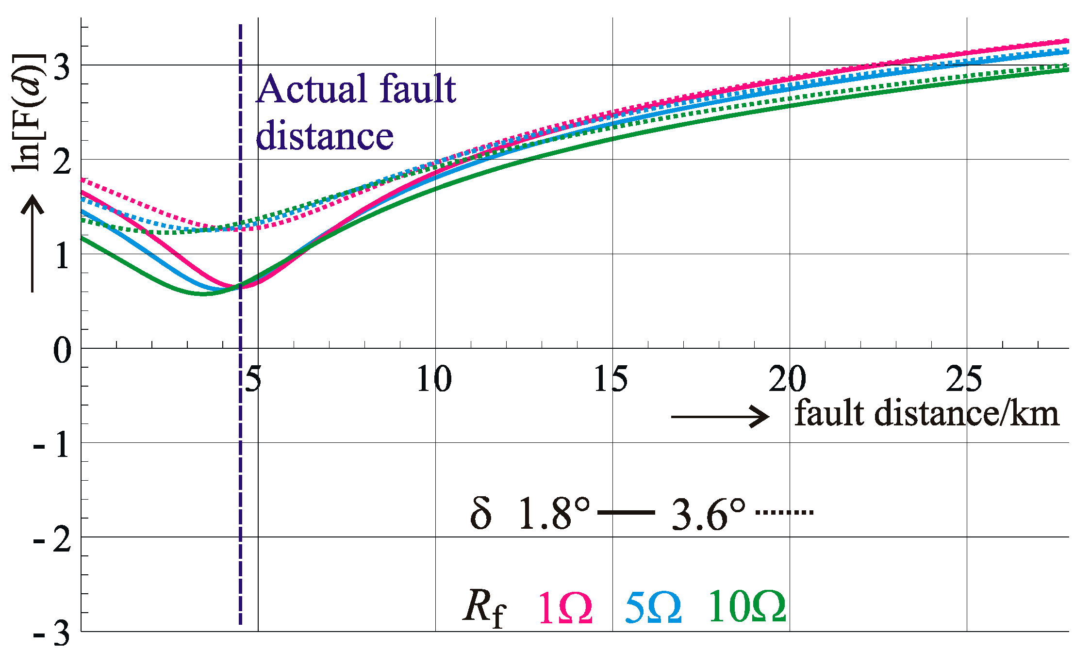
Figure 13.
Testing the synchronization accuracy sensitivity.


Table 1.
Line parameters.
| Positive- and negative-sequence impedance | |
| Zero-sequence impedance | |
| Positive- and negative-sequence admittance | |
| Zero-sequence admittance | |
| Residual compensation factor |
Table 2.
Testing the impact of the fault resistance.
| Fault Resistance | Error of the Calculation at the x-Point Terminal (Fault Distance 4.49 km) | Error of the Calculation at the y-Point Terminal (Fault Distance 23.29 km) | ||||||
|---|---|---|---|---|---|---|---|---|
| Proposed Algorithm | Distance Relay Locator | Proposed Algorithm | Distance Relay Locator | |||||
| (Ω) | (m) | (%) | (m) | (%) | (m) | (%) | (m) | (%) |
| 1 | −9 | 0.2 | 83 | 1.8 | 9 | 0.04 | −694 | 3.0 |
| 5 | −26 | 0.6 | 215 | 4.8 | 26 | 0.1 | −1388 | 5.9 |
| 10 | −27 | 0.6 | 402 | 9.0 | 27 | 0.1 | −2361 | 10.1 |
| 50 | −72 | 1.6 | 2908 | 64.8 | 72 | 0.3 | −13,401 | 57.3 |
| 100 | −128 | 2.9 | 9107 | 202.8 | 128 | 0.5 | −32,156 | 137.5 |
© 2019 by the authors. Licensee MDPI, Basel, Switzerland. This article is an open access article distributed under the terms and conditions of the Creative Commons Attribution (CC BY) license (http://creativecommons.org/licenses/by/4.0/).
Share and Cite
MDPI and ACS Style
Bukvisova, Z.; Orsagova, J.; Topolanek, D.; Toman, P. Two-Terminal Algorithm Analysis for Unsymmetrical Fault Location on 110 kV Lines. Energies 2019, 12, 1193. https://doi.org/10.3390/en12071193
AMA Style
Bukvisova Z, Orsagova J, Topolanek D, Toman P. Two-Terminal Algorithm Analysis for Unsymmetrical Fault Location on 110 kV Lines. Energies. 2019; 12(7):1193. https://doi.org/10.3390/en12071193
Chicago/Turabian StyleBukvisova, Zuzana, Jaroslava Orsagova, David Topolanek, and Petr Toman. 2019. "Two-Terminal Algorithm Analysis for Unsymmetrical Fault Location on 110 kV Lines" Energies 12, no. 7: 1193. https://doi.org/10.3390/en12071193
Note that from the first issue of 2016, this journal uses article numbers instead of page numbers. See further details here.