A Trapezoidal Velocity Profile Generator for Position Control Using a Feedback Strategy


1
Department of Electrical Engineering, Pusan National University, Busan 46241, Korea
2
Department of Mechanical Facility Control Engineering, Korea University of Technology and Education, Cheonan 31253, Chungnam, Korea
*
Author to whom correspondence should be addressed.
Energies 2019, 12(7), 1222; https://doi.org/10.3390/en12071222
Submission received: 4 March 2019
/
Revised: 26 March 2019
/
Accepted: 27 March 2019
/
Published: 29 March 2019
(This article belongs to the Special Issue Control in Power Electronics)
Abstract
:Position control is usually achieved using a position controller and a profile generator. The profile generator produces a desired position trajectory from a position reference and predefined profiles. The position controller forces the actual position to trace the generated position trajectory. A time-based profile generator is the most famous profile generator due to its capability of generating various profiles. However, time base difference in analysis and implementation causes a steady-state error. In order to remove the steady-state error, this paper proposes a novel profile generator for a trapezoidal velocity profile generation. The proposed generator is based on a cascaded P-PI position controller which is designed to trace the position reference. A dynamic range limiter is adopted to provide the acceleration and velocity restrictions which are basic functions for generating the trapezoidal profile. In spite of these restrictions, it cannot make a desired velocity profile only using the limiter because deceleration point is inaccurate. To adjust the deceleration point, a feedback compensator is designed which requires the velocity of the deceleration point. The velocity of the deceleration point is estimated from the initial position error. The compensator moves the deceleration point to the appropriate point which can generate the desired velocity profile. The proposed profile generator can remove the steady-state error, and the position response can be easily adjusted to be either overdamped or underdamped by selecting the two gains appropriately. Several experimental results are presented to verify the usefulness of the proposed generator.
1. Introduction
Position control is a widely used control strategy in many applications such as elevators, machine tools, and robots. In position control, an important issue is how to achieve fast and precise position response. To achieve the desired position response, many papers have proposed various kinds of profiles. A trapezoidal velocity profile has a constant acceleration, velocity and deceleration regions. When the region changes, a large jerk causes vibrations which restrict position accuracy and require additional response time [1,2,3]. S-curve and sinusoidal velocity profiles restrict the jerk to a finite value to reduce the vibrations [3,4,5,6,7,8]. The residual vibrations of the S-curve profile can be reduced by an asymmetrical S-curve (AS-curve) and a high order polynomial S-curve profiles. The AS-curve profile reduces the vibrations with fast acceleration and slow deceleration [9]. The high order polynomial S-curve profile generates a smoother profile by increasing the number of cascaded integrators [1]. However, the trapezoidal velocity profile is one of the popular profiles due to its simple structure and fast response. Studies for overcoming the disadvantages of the profile are still under way [10,11].
Contrary to the many studies about the profile kinds, profile generation methods are still rare. Most papers employ a time-based profile generator as the profile generation method. The time-based profile generator calculates key times at which basic value changes according to the predefined profiles and position reference. Using the key times and predefined profile, a basic value profile is generated. Then, the other profiles are produced step by step by using integral operations. In the trapezoidal velocity profile, the basic profile is a jerk profile. From the jerk profile, acceleration, velocity and position profiles are produced. This method is suitable for generating various profiles by increasing the number of key times. However, this method also has a disadvantage caused by the time base difference [12]. Normally, the key time of the time-based profile generator is considered to be a continuous time when a profile is designed mathematically. But the key time can be represented only as a discrete time when the profile is implemented in a real hardware system. This causes an error between the position reference generated by the profile generator and the input reference. This error is difficult to be removed by the time-based profile generator. The profile generators in [13,14] remove the reference error by changing the profile generation method. In deceleration region, the profile generator is switched over to a distance-based profile generator from the time-based generator. The distance-based profile generator can remove the reference error. However, this method increases the complexity of the generator and causes a discontinuous problem at changing from the time-based to the distance-based. In [15], a profile generator based on the three-dimensional state-space is proposed for time-optimal control. Because the state-space includes the actual position, the generator can remove the reference error. But the method is designed to produce a profile which is similar to the S-curve profile.
To remove the reference error of the time-based profile generator for producing the trapezoidal profile, this paper proposes a novel profile generator based on a cascaded P-PI position controller. The controller can trace the position reference without a position error, but it does not provide acceleration restriction. Only, velocity restriction is supported by a limiter. To add acceleration restriction, a limiter with a dynamically changing restriction range is introduced. Although the limiter can keep the maximum value of acceleration within a predefined value, it does not make the desired velocity profile. An unwanted velocity profile is generated from the difference between the deceleration ratio of the P-position controller and the dynamic range limiter. For matching the deceleration ratios, a compensator is designed using the mathematical analysis. The compensator needs the velocity reference of the limiter and the velocity of the deceleration start point. The reference can be easily obtained by using a feedback scheme. But the velocity of the deceleration start point is unknown. It is possible to estimate the velocity from the initial position error. The proposed method can make the desired trapezoidal velocity profile with no position and reference error. In addition, the compensation and estimation gains can change the response characteristics. An overdamped response is suitable for a smooth landing. The fast response time can be achieved with an underdamped response. The feasibility of the proposed profile generator is shown by several experimental results.
2. Trapezoidal Velocity Profile Using a Time-Based Profile Generator
The trapezoidal velocity profile has a constant acceleration, velocity and deceleration. As shown in Figure 1a, in the constant acceleration region, the acceleration is the maximum positive value, ammax, until the velocity reaches the maximum value, ωmmax. After the constant velocity region where the acceleration and velocity are zero and the maximum value respectively, the velocity decreases to zero with the maximum deceleration, −ammax. However, the profile sometimes has to be a triangular velocity profile depending on the magnitude of the position reference. If the magnitude of the position reference is not large enough, the constant velocity region is not only unnecessary but also the acceleration and deceleration regions are shortened. Hence, the profile consisting of only the constant acceleration and deceleration regions has a triangular shape as shown in Figure 1b.
When implementing the trapezoidal velocity profile using the time-based profile generator, the time of the constant acceleration and velocity regions, tacc and tconst, should be controlled precisely. According to the times, the profile divides into the three regions and outputs the maximum acceleration, deceleration, or zero value as acceleration. From the acceleration output, the velocity and position profiles are generated by integration operations. Normally, these times are calculated from the position reference, θm*, as follows:
However, these times are not accurately implemented due to the difference in time bases. The calculation is based on the continuous time, whereas the implementation uses the discrete time. The implementable time has to be represented with a control period and a positive integer because the controller estimates the time by counting the number every control period. Hence, the ideally calculated times must be converted into the implementable times as (3) and (4). In this step, it is inevitable that time errors occur.
where Tacc and Tconst are the time of the constant acceleration and velocity regions on the discrete time base, respectively. Ts means the control period. Δtacc and Δt′const are the time errors resulting from the rounding. t′const is the time of the constant velocity region on the continuous time base when the acceleration region time is Tacc. Then, t′const is defined as follow:
The critical problem which can be caused by the time errors is a position reference disturbance in steady-state. The velocity and position profiles of the time-based profile generator entirely depend on the acceleration profile. It means that the errors of the acceleration profile lead to errors of the velocity and position profiles. In aspect of position control, the velocity profile errors such as slightly exceeding the maximum value are tolerable. But the position profile errors are not neglectable for precise position control. The steady-state position reference of the generator, θm_tb*, is represented as the maximum acceleration and the time of the constant acceleration and velocity regions. From (3)–(5) and the equation about the steady-state position reference, a reference error is derived as follow:
Since the time errors are determined by the input position reference, the maximum velocity and acceleration, it is difficult to know the reference error without the specific value of these parameters. But the maximum reference error which can occur regardless of the parameters is able to obtained. In (3) and (4), it is well known that the rounding makes a difference of up to 0.5 between the input and output. It means that the maximum magnitude of the time error is half of the control period, Ts/2. When the half of the control period substitutes for the time errors, the maximum magnitude of the possible reference error is obtained as (7). Usually, the constant acceleration region time is much larger than the control period. Then, ammaxTs2/4 is negligible and the maximum possible reference error is only proportional to the maximum velocity and control period.
The condition for the triangular velocity profile generation is derived from (4). The constant velocity region time must be larger than zero to maintain the trapezoidal shape. Therefore, if the condition in (8) is satisfied, the generator produces the triangular velocity profile.
The constant acceleration region times on the continuous and discrete time bases are represented by (9) and (10) respectively. In a similar manner to the analysis about the reference error of the trapezoidal velocity profile, the reference error and the maximum possible reference error are derived as (11) and (12). The maximum possible reference error of the triangular profile is also proportional to the velocity and control period as given by (12).
where t′acc and T′acc are the constant acceleration region times of the triangular profile on the continuous and discrete time base, respectively. Δt′acc is the acceleration region time error.
Figure 2 shows the reference error calculated from (3), (4), and (9) and the maximum possible reference error of (7) and (12) when the control period, the maximum velocity and acceleration are 100 [us], 2000 [rpm], and 10,000 [rpm/s] respectively. The detail values of the reference error are not distinguished, but the error does not exceed the maximum possible error. Until the position reference of 2400 [deg], the profile has the triangular shape. The maximum error of the triangular profile is not fixed to one value because the velocity at t′acc varies depending on the position reference. The larger position reference, the larger maximum error. If the velocity at t′acc has the maximum value, the maximum possible error is the largest among the errors of the trapezoidal and triangular profiles. The maximum possible error of the trapezoidal profile is half of the largest error in the triangular profile. In conclusion, using the time-based profile generator can be limited for some applications which require high position accuracy. To increase the position accuracy of the generator, the maximum velocity, control period, or both should be reduced. However, the reduction of the maximum velocity increases the position response time. And, the control frequency is limited by the hardware performance.
3. Proposed Velocity Profile Generator
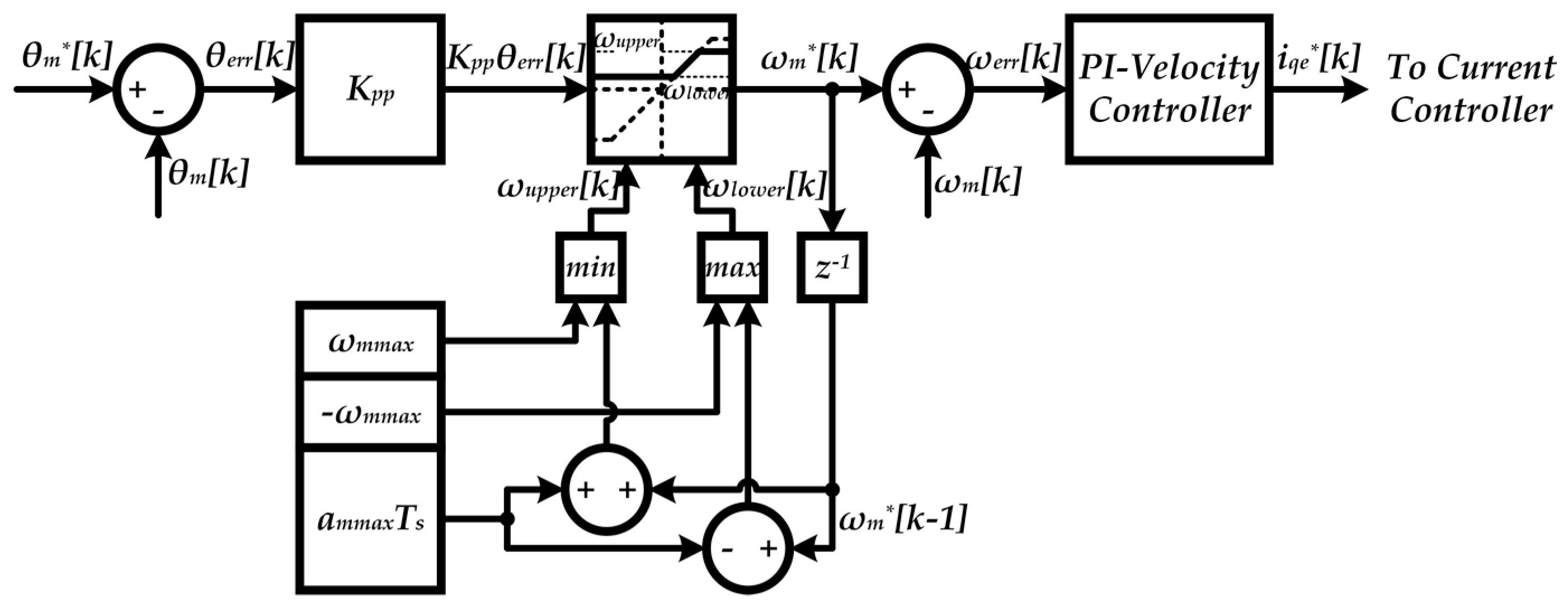
In this paper, a novel profile generator based on the conventional cascaded P-PI position control is proposed. Although the convention P-PI position controller [16] does not make any specific profile, it can trace the position reference without position error. The conventional P-PI controller includes a limiter which is located between the P-position controller and PI-velocity controller to prevent the over velocity. In this scheme, the easiest way to restrict the acceleration within the maximum value is to replace the limiter with a dynamic range limiter as shown in Figure 3. The upper and lower limitation value, ωupper and ωlower, are defined as (13). When the velocity reference does not exceed the maximum value, this limiter operates as the acceleration limiter by increasing or decreasing the velocity reference within the predefined constant ratio. In addition, it can provide the velocity limitation by restricting the value of the upper and lower limit to the maximum velocity.
where ωm* is the velocity reference. k and k − 1 mean the current and previous control points.
However, even if the dynamic range limiter operates well as the acceleration and velocity limiters, the generated velocity shape may be different from the desired velocity profile. In the constant acceleration region, the velocity reference just increases with the maximum acceleration because the position controller output is much larger than the velocity reference. But, in the constant deceleration region, the position controller output converges to zero and conversion speed decides the profile shape. If the position controller output changes faster than the velocity reference, the position overshoot occurs as shown in Figure 4a. In the worst case, the position does not converge to the reference and it may even diverge. On the other hands, Figure 4b shows the velocity profile when the position controller output changes slowly. Since the velocity reference follows the output of the P-controller at the end of the deceleration region, additional time is needed to reach the position reference.
When the average deceleration ratio of the position controller output is the maximum value during the deceleration region, it is possible to generate the desired velocity profile as shown in Figure 5. The position controller output matches the velocity reference at the deceleration start time, tdec, and reaches zero at the settling time, tset. The velocity reference decreases to zero with the constant ratio and keeps zero after reaching zero. The desired velocity reference during the deceleration region can be represented by (14). And, a condition for making the desired profile can be derived from (14).
where tdec and tset are either tconst + tacc or t′acc, tconst + 2tacc or 2t′acc in Figure 1, depending on the profile kinds.
The position error, θerr, which is an input to the position controller can be derived from (14) as follow:
At the deceleration start time, the position controller output is same as the velocity reference. Hence, the proportional gain of the position controller for the desired profile, Kpp0, is derived as (16). The maximum acceleration value is determined considering the system requirements. The velocity reference at the deceleration start time is determined by the position reference. In result, the controllable parameter is only the proportional gain of the position controller, Kpp. However, because the proportional gain affects the position response characteristics, it is also hard to determine the proportional gain with the value of (16).
Assuming that the velocity reference is fixed as the desired shape, the position controller outputs according to the proportional gains can be drawn as the waveform of Kpp1 or Kpp2 in Figure 5. A larger or smaller gain makes the deceleration start time to be delayed or advanced than the desired time. This time mismatch causes the unwanted velocity shape as mentioned above. In order to generate the desired profile, the waveforms of Kpp1 and Kpp2 have to be redrawn as the waveform of Kpp0 using some compensations. And, the compensated position controller output must satisfy following two conditions. The first condition of (17) represents about the deceleration start time. At the deceleration start time, the compensated output should be the same as the velocity reference. The other is related to the constant deceleration. To keep the maximum deceleration, the compensated output should be less than or equal to the velocity reference during the deceleration.
where ωmcom* and ωmfb are the compensated position controller output and the compensation velocity, respectively.
From the two conditions and (15), the compensation velocity can be defined as follow:
The compensation velocity is related to the proportional gain of (16). Equation (19) can be rewritten as (20) using (15) and (16). The compensation velocity ideally removes the difference in the position controller output caused by the difference between the proportional gain and the required gain, and makes the compensated position controller output same as the output which can generate the desired velocity profiles. But it does not mean that the proportional gain is useless. The ideal trapezoidal or triangular profile on the discrete time base must have the steady-state error as same reason of the time-based generator. To remove the steady-state error, the velocity profile requires one more region which is called approach region in this paper. Hence, although the velocity profile could be hard to distinguish from the ideal profiles, the exact velocity profile is similar to one of the velocity shapes in Figure 4. The proportional gain decides the response characteristics of the approach region.
The deceleration start time and the velocity at that time of (19) are unknown. And the velocity must be required for the compensation. If the profile is the triangular profile, it can be obtained as (21) from (15). Especially, from the fact that the position variation of the acceleration and deceleration regions are the same, the velocity can be represented with the initial position error, θerr(0). In the trapezoidal profile, the velocity is the maximum value and the estimated velocity of (21) is wrong. But it is obvious that the estimated velocity is larger than the maximum value. Hence, the velocity at the deceleration start time can be estimated as (22) regardless of the profile kinds.
Figure 6 shows the P-position controller including the proposed profile generation method. The initial position error is held when the position reference change is detected. From the initial position error and (22), the velocity at the deceleration start time is estimated. The estimated velocity and (19) consist of the main compensator.
The gains of the estimator and compensator, Kest and Kcom, are ideally 1. But the gains have to be adjusted experimentally due to some errors caused by the velocity response characteristics and the time base difference. The gains can determine the position response characteristics. Ideally, when the gains are larger than 1, the deceleration start time occurs early and the position response is underdamped. On the contrary, small gains make overdamped position response.
4. Experimental Results
Some experiments for verifying the effectiveness of the proposed profile generator are performed with the experimental setup as shown in Figure 7. Only the second back to back converter and Surface mounted Permanent Magnet Synchronous Motor (SPMSM) are used. The specifications of SPMSM are listed in Table 1. The overall control algorithms are implemented using TMS320C28346 microcontroller manufactured by Texas Instruments (Texas Instruments, Dallas, TA, USA). The switching frequency and the current control frequency including the conventional time-based profile generator are 10 [kHz]. And, the control frequency for the cascaded P-PI position controller is 1 [kHz]. The maximum velocity and acceleration are 2000 [rpm] and 10,000 [rpm/s], respectively, which are same as the conditions of Figure 2.
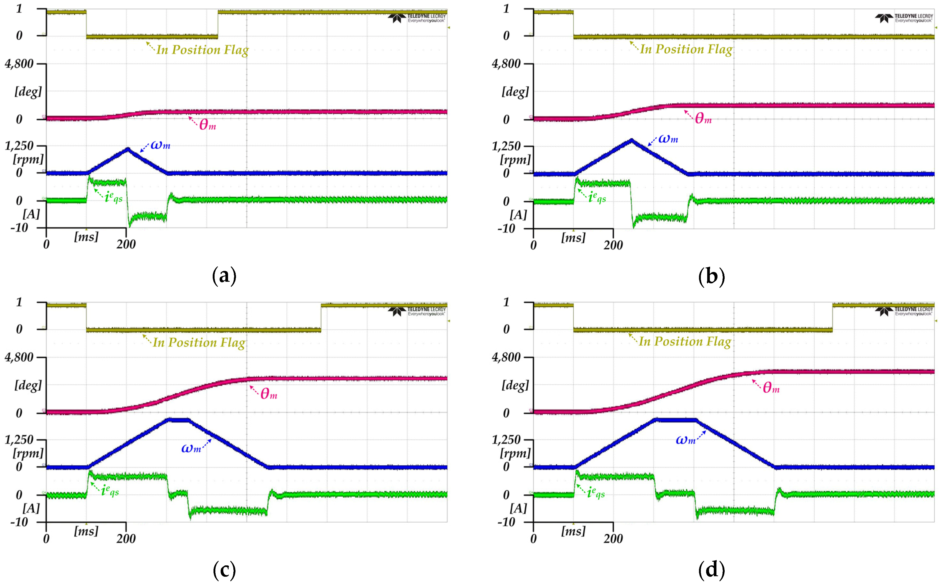
Figure 8 shows the position, velocity and q-axis current of the time-based profile generator. “In Position Flag” means that the absolute value of the error between the position reference and the actual position is less than 0.225 [deg] corresponding to 5 pulses of the encoder. The position reference is inputted at 100 [ms]. Then, the position error exceeds the allowable position error, 0.225 [deg], and “In Position Flag” is cleared to 0. When the position references are 600 [deg] and 1200 [deg], the velocity trajecories show the triangular shapes as shown in Figure 8a,b. In the acceleration and deceleration regions of the triangular profile, the magnitude of the q-axis current is 7[A] and almost flat. The velocity increases with the constant ratio. In Figure 8a, the actual position is considered to reach the position reference because the position error is less than the allowable position error after 430 [ms], when “In Position Flag” returns to 1. However, in the case of Figure 8b, the flag remains 0 and it means the actual position cannot reach within the range of “In Position”. The trapezoidal velocity profile occurs when the position references are 3000 [deg] and 3600 [deg] as shown in Figure 8c,d. The control results are similar with the results of the triangular profile except for the constant velocity region. The velocity of the trapezoidal profile increases to the maximum velocity and keeps the maximum velocity for a moment. The time of the constant velocity region varies depending on the position reference. The transient response time of 3000 [deg] and 3600 [deg] are 580 [ms] and 640 [ms], respectively. The actual position of the two cases reach the references.
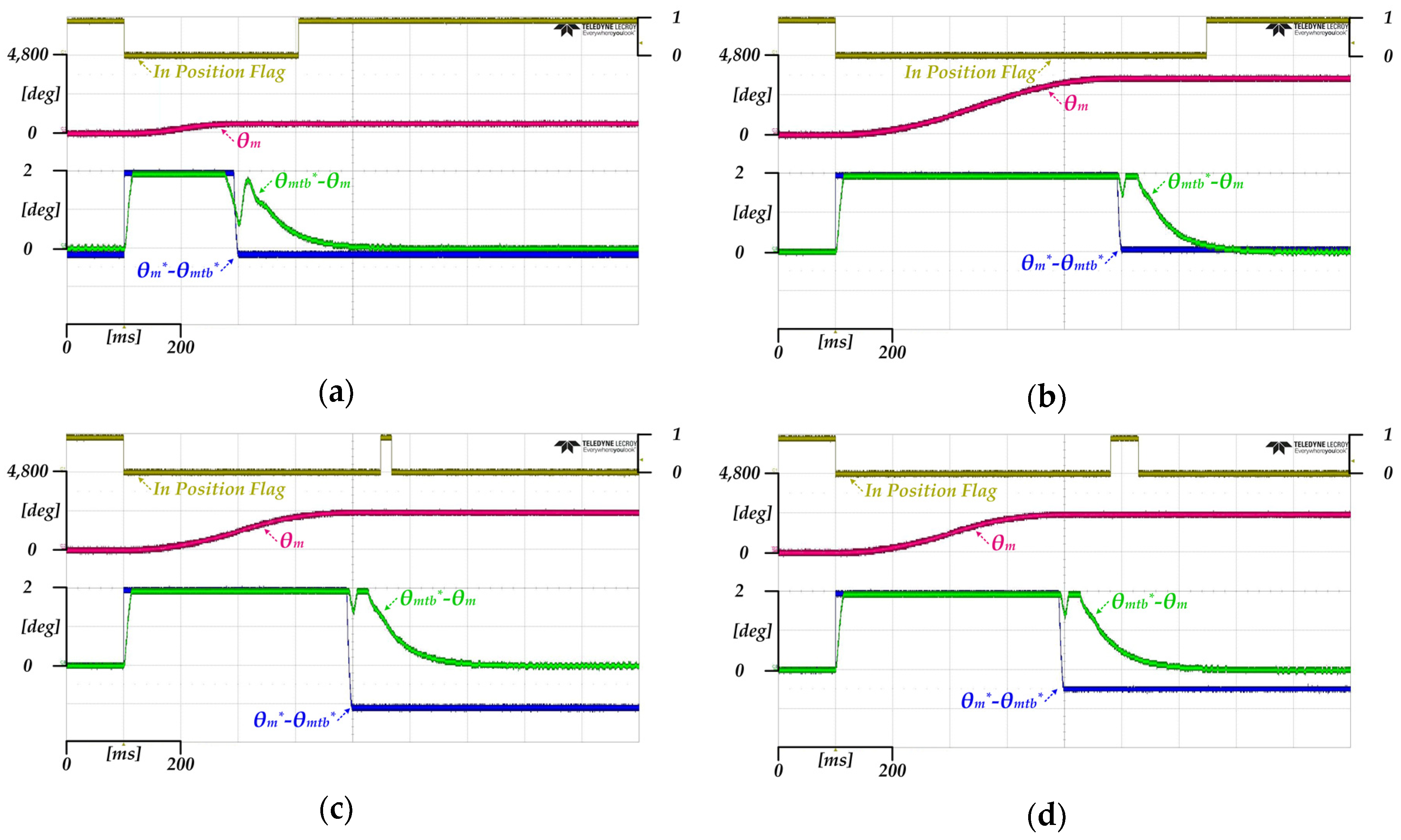
The reason why the actual position of 1200 [deg] reference does not reach to the position reference is shown in Figure 9. The errors exceeding 2 [deg] are represented as 2 [deg] in Figure 9. The position errors, θmtb* − θm, between the position reference generated by the time-based generator and the actual position converge to 0 regardless of the input position reference. As a result, the position controller can trace the generated reference. But, the reference errors, θm* − θmtb*, between the input position reference and the generated position reference are different depending on the input reference. As show in Figure 9a, when the input reference is 1200 [deg], the reference error is 0.3589 [deg] which is larger than the allowable position error. On the contrary, the reference error of 3600 [deg] reference is 0.06393 [deg], which is acceptable. It means that the steady-state error is caused by the time-based profile generator. Depending on the input position reference, the reference error can exceed the allowable position error. Under experimental conditions, the largest reference error of the triangular and trapezoidal profiles occur when the position references are 2398.9 [deg] and 2400.7 [deg], respectively. From the mathematical analysis, the largest reference errors are 1.2 [deg] and 0.6 [deg] for these references. And, the actual reference errors are 1.108 [deg] and 0.5082 [deg] as shown in Figure 9c,d, which is similar to the analytical value. Hence, even if the position controller works well, the reference error can be caused by the time-based profile generator as mentioned in Section 2.
The proposed method uses the compensator for matching the response characteristics of the position controller and the limiter. When the proportional gain of the controller is too large for the fast response, the limiter cannot follow the controller output. In Figure 10, the controller output, Kppθerr, is too rapid to generate the desired profile. Before the compensation, the velocity would start to decrease at 310 [ms]. And, it generates an underdamped response. But after the compensation, the velocity starts to decrease at 250 [ms]. The compensated output, ωmcom*, changes slowly which is enough to generate the triangular shape. At the end of the deceleration region, the approach region exists. In this region, the velocity and compensated output trace the position controller output.
The control results of the proposed method are shown in Figure 11 when the position references are same as Figure 8. The compensation and estimation gains are adjusted to make an overdamped response. The velocity shapes of the proposed method are very similar to the conventional method except the approach region. In Figure 11a, after 300 [ms], the velocity does not decrease directly to 0 but approaches 0 smoothly. The q-axis current also slowly increases to 0 after increasing to −2.5 [A] rapidly. This velocity and current waveforms are shown in the other figures. By the overdamped response, additional response times of about 30 [ms] are required than the conventional method for all references. The proposed method can produce a velocity profile which is similar to the original profile and is able to reach the reference smoothly. By the conventional profile generator, the actual position does not reach the reference of 1200 [deg]. But, as shown in Figure 11b, the actual position of the proposed method can reach the position reference. In cases of the trapezoidal profile as shown Figure 11c,d, the proposed profile generator can produce the desired profile. Also, the actual positions reach the references. The characteristics of the approach region are maintained regardless of the magnitude of the position reference.
Figure 12 also shows the control results of the proposed method. But the compensation and estimation gains are decided for an underdamped response. In Figure 12a, the time of the constant acceleration region is several milliseconds longer than the time of Figure 11a. The time increase of the deceleration region is enough large to be distinguished. As the time increase of the deceleration region is larger than the time increase of the acceleration region, the velocity decreases to a negative value. It means the position overshoot occurs. “In Position Flag” of Figure 12a returns to 1 by three times. For the first time, the actual position reaches the reference at 290 [ms]. But the actual position exceeds the reference because the velocity is not 0 and is a positive value. The second occurs at 350 [ms] when the velocity is a negative value. So, the actual position moves down the reference. When the actual position converges to the reference, the flag is set to 1 finally. The characteristics of the other references in Figure 12b–d are little different. In these cases, the flag must return to 1 by two times. The first has to occur in the same situation as at 350 [ms] in Figure 12a. However, the controller does not detect because the position passes the range of “In Position” too fast. So, Figure 12b–d just show the flag waveforms which only return to 1 once. In conclusion, about 40 [ms] response time is reduced from the time of the overdamped response when the position reference is 600 [deg]. It is similar to the conventional method. In Figure 12b–d, the response time is about 70 [ms] shorter than the overdamped response and is about 30 [ms] shorter than the conventional method. The actual positions can reach the position references, even though the response is underdamped.
5. Conclusions
The time-based profile generator is widely used because it can provide the powerful solution for producing various profile kinds. However, the time base difference of the analysis and implementation reduced the position precision. The prediction of the exact position error was impossible without specifications of the system operation. The maximum possible position error was obtained from the control period and velocity. To remove the position error, this paper proposed the novel profile generator based on the cascaded P-PI position controller and the dynamic range limiter. When only the position controller and limiter were used, the proportional gain of the position controller must be selected as an appropriate value depending on the position reference and the maximum acceleration value. The compensator which has the feedback scheme including the velocity estimator could generate the compensated output for the desired profile regardless of the proportional gain. The proposed profile generator produced the triangular and trapezoidal profile without the steady-state error. The compensation and estimation gains could decide the position response to be the underdamped or overdamped. If the gains were determined for the overdamped response, the additional time was required. But smooth landing was possible. The gains for the underdamped response caused the disadvantages such as the position overshoot and rapid current change. It was possible to reduce the response time. The feasibility of the proposed profile generator was confirmed by several experimental results.
Author Contributions
Conceptualization, J.-M.K.; formal analysis, visualization and writing—original draft preparation, H.-J.H.; validation, Y.S.; writing—review and editing, Y.S. and J.-M.K.; project administration, J.-M.K.
Acknowledgments
This research was supported by the Basic Science Research Program through the National Research Foundation of Korea (NRF) funded by the Ministry of Education (NRF-20188R1D1A1B07048954).
Conflicts of Interest
The authors declare no conflict of interest.
References
- Nguyen, K.D.; Ng, T.-C.; Chen, I.-M. On Algorithms for Planning S-curve Motion Profiles. Int. J. Adv. Robot. Syst. 2008, 5, 99–106. [Google Scholar] [CrossRef]
- Ha, C.-W.; Rew, K.-H.; Kim, K.-S. Robust Zero Placement for Motion Control of Lightly Damped Systems. IEEE Trans. Ind. Electron. 2013, 60, 3857–3864. [Google Scholar] [CrossRef]
- Meckl, P.H.; Arestides, P.B. Optimized S-Curve Motion Profiles for Minimum Residual Vibration. In Proceedings of the 1998 American Control Conference, Philadelphia, PA, USA, 26 June 1998; pp. 2627–2631. [Google Scholar] [CrossRef]
- Shin, S.-C.; Choi, C.-H.; Youm, J.-H.; Lee, T.-K.; Won, C.-Y. Position Control of PMSM using Jerk-Limited Trajectory for Torque Ripple Reduction in Robot Applications. In Proceedings of the IECON 2012—38th Annual Conference on IEEE Industrial Electronics Society, Montreal, QC, Canada, 25–28 October 2012; pp. 2400–2405. [Google Scholar] [CrossRef]
- Arelavo, V.M. Sinusoidal Velocity Profiles for Motion Control. In Proceedings of the ASPE Control of Precision Systems, Philadelphia, PA, USA, 18–20 April 2001. [Google Scholar]
- Li, H.Z.; Gong, Z.; Lin, W.; Lippa, T. A New Motion Control Approach for Jerk and Transient Vibration Suppression. In Proceedings of the 2006 4th IEEE International Conference on Industrial Informatics, Singapore, 16–18 August 2006; pp. 676–681. [Google Scholar] [CrossRef]
- Li, H.; Le, M.D.; Gong, Z.M.; Lin, W. Motion Profile Design to Reduce Residual Vibration of High-Speed Positioning Stages. IEEE/ASME Trans. Mechatron. 2009, 14, 264–269. [Google Scholar] [CrossRef]
- Jeon, J.W.; Ha, Y.Y. A Generalized Approach for the Acceleration and Deceleration of Industrial Robots and CNC Machine Tools. IEEE Trans. Ind. Electron. 2000, 47, 133–139. [Google Scholar] [CrossRef]
- Tsay, D.-M.; Lin, C.-F. Asymmetrical Inputs for Minimizing Residual Response. In Proceedings of the IEEE International Conference on Mechatronics, Taipei, Taiwan, 10–12 July 2005; pp. 235–240. [Google Scholar] [CrossRef]
- Minárech, P.; Vittek, J.; Vavrúš, V.; Makyš, P. Experimental Verification of New Energy Saving Position Control Algorithm for AC Drives. In Proceedings of the 2012 ELEKTRO, Rajecké Teplice, Slovakia, 21–22 May 2012; pp. 216–220. [Google Scholar] [CrossRef]
- Yoon, H.J.; Chung, S.Y.; Kang, H.S.; Hwang, M.J. Trapezoidal Motion Profile to Suppress Residual Vibration of Flexible Object Moved by Robot. Electronics 2019, 8, 30. [Google Scholar] [CrossRef]
- Beldiman, O.V.; Wang, H.O.; Bushnell, L.G. Trajectory Generation of High-Rise/High-Speed Elevators. In Proceedings of the 1998 American Control Conference, Philadelphia, PA, USA, 26 June 1998; pp. 3455–3459. [Google Scholar] [CrossRef]
- Ryu, H.-M.; Sul, S.-K. Position Control for Direct Landing of Elevator using Time-based Position Pattern Generation. In Proceedings of the 2002 IEEE Industry Applications Conference, Pittsburgh, PA, USA, 13–18 October 2002; pp. 644–649. [Google Scholar] [CrossRef]
- Kei, T.W.; Mang, V.; Un, C.S. Design of S-curve Direct Landing Position Control System for Elevator using Microcontroller. In Proceedings of the World Congress on Engineering and Computer Science, San Francisco, CA, USA, 24–26 October 2012. [Google Scholar]
- Kim, Y.-O.; Ha, I.-J. Time-Optimal Control of a Single-DOF Mechanical System Considering Actuator Dynamics. IEEE Trans. Control Syst. Technol. 2003, 11, 919–932. [Google Scholar] [CrossRef]
- Sul, S.-K. 4.4 Position Regulator. In Control of Electric Machine Drive Systems; EI-Hawary, M.E., Ed.; Wily: Hoboken, NJ, USA, 2011; pp. 208–209. [Google Scholar]
Figure 1.
The acceleration, velocity and position profiles: (a) the trapezoidal velocity profile; (b) the triangular velocity profile.
Figure 1.
The acceleration, velocity and position profiles: (a) the trapezoidal velocity profile; (b) the triangular velocity profile.

Figure 2.
The position error and the maximum possible position error with the specific parameters.

Figure 3.
The block diagram of the cascaded P-PI controller on the discretized time base with the dynamic range limiter for the acceleration and velocity limitation.
Figure 3.
The block diagram of the cascaded P-PI controller on the discretized time base with the dynamic range limiter for the acceleration and velocity limitation.

Figure 4.
A velocity and position profiles generated by the dynamic range limiter: (a) a fast output change of the position controller; (b) a slow output change of the position controller.
Figure 4.
A velocity and position profiles generated by the dynamic range limiter: (a) a fast output change of the position controller; (b) a slow output change of the position controller.

Figure 5.
The output of the position control according to the proportional gain when the velocity profile is the desired shape.
Figure 5.
The output of the position control according to the proportional gain when the velocity profile is the desired shape.

Figure 6.
The position controller including the proposed profile generator.

Figure 7.
Back to back converter and motor-generator set for experimentation.

Figure 8.
Position, velocity and q-axis current of the conventional time-based profile generator (a) 600 [deg] position reference; (b) 1200 [deg] position reference; (c) 3000 [deg] position reference; (d) 3600 [deg] position reference.
Figure 8.
Position, velocity and q-axis current of the conventional time-based profile generator (a) 600 [deg] position reference; (b) 1200 [deg] position reference; (c) 3000 [deg] position reference; (d) 3600 [deg] position reference.

Figure 9.
The reference error and position error (a) 1200 [deg] position reference; (b) 3600 [deg] position reference; (c) 2398.9 [deg] position reference; (d) 2400.7 [deg] position reference.
Figure 9.
The reference error and position error (a) 1200 [deg] position reference; (b) 3600 [deg] position reference; (c) 2398.9 [deg] position reference; (d) 2400.7 [deg] position reference.

Figure 10.
The position controller output, compensated output and actual velocity of the proposed method.
Figure 10.
The position controller output, compensated output and actual velocity of the proposed method.

Figure 11.
Position, velocity and q-axis current of the proposed method under the overdamping condition (a) 600 [deg] position reference; (b) 1200 [deg] position reference; (c) 3000 [deg] position reference; (d) 3600 [deg] position reference.
Figure 11.
Position, velocity and q-axis current of the proposed method under the overdamping condition (a) 600 [deg] position reference; (b) 1200 [deg] position reference; (c) 3000 [deg] position reference; (d) 3600 [deg] position reference.

Figure 12.
Position, velocity and q-axis current of the proposed method under the underdamping condition (a) 600 [deg] position reference; (b) 1200 [deg] position reference; (c) 3000 [deg] position reference; (d) 3600 [deg] position reference.
Figure 12.
Position, velocity and q-axis current of the proposed method under the underdamping condition (a) 600 [deg] position reference; (b) 1200 [deg] position reference; (c) 3000 [deg] position reference; (d) 3600 [deg] position reference.


Table 1.
Motor specifications.
| Surface Mounted Permanent Magnet Synchronous Motor (SPMSM) | ||
|---|---|---|
| Parameters | Unit | Value |
| Rated Power | kW | 2.2 |
| Rated Speed | rpm | 3000 |
| Rated Current | A | 17 |
| Back-Electromotive Force (Back-EMF) Constant | V/krpm | 28.75 |
| Pole Pairs | - | 4 |
| Stator Resistance | mΩ | 210 |
| Stator Inductance | mH | 1.55 |
| Pulses per Revolution (PPR) of Encoder | - | 8000 |
© 2019 by the authors. Licensee MDPI, Basel, Switzerland. This article is an open access article distributed under the terms and conditions of the Creative Commons Attribution (CC BY) license (http://creativecommons.org/licenses/by/4.0/).
Share and Cite
MDPI and ACS Style
Heo, H.-J.; Son, Y.; Kim, J.-M. A Trapezoidal Velocity Profile Generator for Position Control Using a Feedback Strategy. Energies 2019, 12, 1222. https://doi.org/10.3390/en12071222
AMA Style
Heo H-J, Son Y, Kim J-M. A Trapezoidal Velocity Profile Generator for Position Control Using a Feedback Strategy. Energies. 2019; 12(7):1222. https://doi.org/10.3390/en12071222
Chicago/Turabian StyleHeo, Hong-Jun, Yungdeug Son, and Jang-Mok Kim. 2019. "A Trapezoidal Velocity Profile Generator for Position Control Using a Feedback Strategy" Energies 12, no. 7: 1222. https://doi.org/10.3390/en12071222
Note that from the first issue of 2016, this journal uses article numbers instead of page numbers. See further details here.