Large-Eddy Simulation-Based Study of Effect of Swell-Induced Pitch Motion on Wake-Flow Statistics and Power Extraction of Offshore Wind Turbines


Department of Mechanical Engineering, University of Houston, Houston, TX 77004, USA
*
Author to whom correspondence should be addressed.
Energies 2019, 12(7), 1246; https://doi.org/10.3390/en12071246
Submission received: 12 March 2019
/
Revised: 24 March 2019
/
Accepted: 25 March 2019
/
Published: 1 April 2019
(This article belongs to the Section A3: Wind, Wave and Tidal Energy)
Abstract
:In this study, the effects of ocean swell waves and swell-induced pitch motion on the wake-flow statistics and power extraction of floating wind turbines are numerically investigated. A hybrid numerical model coupling wind large-eddy (LES) and high-order spectral-wave simulations is employed to capture the effects of ocean swell waves on offshore wind. In the simulation, floating wind turbines with prescribed pitch motions were modeled using the actuator disk model. The turbulence statistics and wind-power extraction rate for the floating turbines are quantified and compared to a reference case with fixed turbines. Statistical analysis based on the phase-average approach shows significant swell-correlated wind-velocity variations in both cases, and the swell-induced pitch motion of floating turbines is found to cause oscillations of wind-turbulence intensity and Reynolds stress, as well as an increase of vertical velocity variance in the near-wake region. Swells also cause periodic oscillation in extracted power density in the fixed turbine case, and the turbine pitch motion in the floating turbine case could further modulate this oscillation by shifting the phase dependence by about 180 degrees with respect to the swell-wave phase.
1. Introduction
The continuous growth of global energy consumption has imposed great challenges on energy supply. In recent years, wind energy has been playing a vital role in providing clean and renewable energy to fulfil demands without generating major adverse impact on the environment like other conventional energy sources based on fossil fuels [1]. As available and suitable land spaces for building onshore wind farms are limited, offshore wind power is becoming an emerging direction for future wind-energy research [2,3]. Without resistance caused by ground obstacles like in onshore environments, offshore wind in the marine atmospheric boundary layer (ABL) usually possesses higher wind speed than its onshore counterpart, offering higher wind-power density for energy harvesting. On the other hand, marine ABL turbulence also exhibits complex flow phenomena in its lower portion where the wind and sea-surface waves extensively interact, imposing considerable challenges to the design of individual offshore wind turbines, as well as large offshore wind farms.
The characteristics of offshore wind are highly affected by the dynamic interactions between wind turbulence and progressive sea-surface waves in the marine ABL [4,5]. For wind-energy applications, local wind-generated broadband sea-surface waves (often called the wind sea) can be regarded as moving surface-roughness elements that affect the lower portion of the ABL through effective surface friction [6,7]. In addition, long-wavelength swell waves generated by remote storm events can maintain their long-crest shapes after propagating over long distances and impact the local flow field in offshore environments [8,9]. Due to the their well-organized wave forms and large-surface orbital velocities (associated with their long wavelength of and fast phase speed of ), swell waves can induce strong distortions to the near-surface wind field that can extend up to the height of [8]. Considering wind–wave coupled dynamics is crucial for understanding the offshore wind-power resource and predicting the performance of offshore wind turbines.
In addition to modulating the offshore wind field, energetic swell waves can also cause considerable oscillating motions for floating turbine platforms, which further complicates the dynamics of offshore wind-energy systems and affects their performance. Recently, Rockel et al. [10,11] performed laboratory experiments using a wind-turbine model installed on a gimbal support to study the effect of turbine pitch motion on wake-flow statistics. Using the particle-image velocimetry technique, they measured and quantified the turbulence statistics in the turbine wake. Although the effects of water waves on wind were not included in their experiment, the experimental data showed considerable effects of the turbine pitch motion on wake-flow statistics. Using the free-vortex method, Wen et al. [12] studied the power extraction of a single floating turbine and found considerable influence of the platform pitch motion on the floating turbine’s power performance. Despite the improved understanding of the pitch-motion effects on the performance and structure dynamics of a single wind turbine, the effects of turbine pitch motion on the flow structures and turbine performance in an offshore wind-farm environment are still not well-understood.
In recent years, the large-eddy simulation (LES) method combined with the actuator-disk model (ADM) of the wind turbine has become a valuable tool for studying flow physics in the turbulent flow behind a single turbine [13], or within large wind farms [14]. For example, Calaf et al. [15,16] performed pioneering studies using LES and ADM to simulate complex turbulent-flow physics, vertical kinetic-energy entrainments, and scalar transport in fully developed wind-turbine array boundary layer. Stevens et al. [17] performed a set of LES runs to quantify the effects of turbine alignment and wind-farm length on turbine performance within a large wind farm. Stevens and Meneveau [18] investigated the temporal fluctuations of the wind-power extraction rate based on LES data of extended wind farms. VerHulst and Meneveau [19] performed extensive statistical analyses of LES data for wind farms using the three-dimensional proper orthogonal decomposition approach, and identified various large coherent flow structures at the wind-turbine array scale that are associated with vertical kinetic-energy entrainments to supply wind energy into the wind-turbine arrays in the middle of very large wind farms. Yang et al. [20] simulated infinite aligned wind farms with various turbine spacings to quantify the effects of turbine packing density on wind-energy harvest. Yang and Sotiropoulos [21] studied the effect of staggered turbine layouts on the wind-power extraction of large wind farms. Zhang et al. [22] explored the potential benefit of using vertically staggered turbine layouts to enhance the wind-power production of a turbine array. Yang et al. [7,9] coupled LES with a wave simulation based on the high-order spectral method (HOSM), and studied the effect of wind sea as well as swell waves on flow structures and turbulence in offshore wind farms with fixed turbines. Lyu et al. [23] further extended the model of Yang et al. [7,9] by also adding the actuator-line and actuator-disk models with a rotational effect for the turbines.
In this study, we use the LES–HOSM model of Yang et al. [7,9] to study the effect of swell-induced pitch motion on turbulence statistics and wind-power extraction rate in an array of floating wind turbines. We considered long swell waves that propagate in the downwind direction. The simulations of wind and swell waves are coupled in order to capture strong swell-induced disturbances on the near-surface wind field and their effects on wind-energy extraction. Similar to previous LES studies [15,16], we considered an array of wind turbines in horizontally and vertically aligned layouts. With a periodic boundary condition applied in the horizontal directions, the simulation models the interaction of ABL wind with an “infinite” turbine array, which represents flow physics in the fully developed region within a very large wind farm [14,15]. We simulated the floating turbines with a prescribed periodic pitch motion under the influence of wind and swell-wave forcing, and compared the simulation results with a reference case with identical conditions but fixed turbines. The LES data were analyzed using the phase-average approach by sampling flow-field snapshots at specific phases with respect to the swell-wave form, which allows us to educe swell-correlated turbulence statistics from this complex flow problem. The time series of the wind-power extraction rate were also quantified to reveal the impact of swell-induced wind-speed variation and turbine pitch motion on wind-energy harvesting.
This paper is organized as follows. Section 2 discusses the used model equations and numerical schemes in LES and HOSM. Section 3 shows the data-analysis results for the statistics of the wind turbulence in the turbine array boundary layer and the wind-power extraction rate. Finally, conclusions are given in Section 4.
2. Problem Description and Numerical Methods
2.1. Large-Eddy Simulation Model for Wind Fields
In the LES model, wind-flow motions in a neutral atmospheric boundary layer are simulated by solving the filtered Navier–Stokes equations [7,9,15,17,21]
The model equations are defined based on a regular Cartesian co-ordinate system , where x and y are the horizontal co-ordinates and z is the vertical co-ordinate. The origin of the z co-ordinate was set to be at the mean water level near the instantaneous bottom boundary. In Equations (1) and (2), is the velocity vector, with u, v, and w being the corresponding velocity components in the x-, y-, and z-directions, respectively; the tilde denotes a variable resolved by the LES grid scale; is air density; is the subgrid-scale (SGS) stress tensor with being its trace and being its deviatoric part, where is the identity tensor; is the pseudopressure, with p being the dynamic pressure; is the imposed pressure gradient to model the effect of geostrophic wind forcing [15,16]; is the turbine-induced force on the wind field; and is the unit vector in the x-direction. In Equation (1), the effect of molecular viscosity is neglected because the Reynolds numbers for ABL flows in wind-energy applications are typically quite high, so that the effects of unresolved SGS terms dominate over molecular viscous terms [15]. We note that, for large wind farms, the thermal stability conditions of the ABL can also affect dynamic interactions between wind farms and the ABL flows (e.g., References [24,25]). For the sake of simplicity and to allow us focus on studying the effect of sea-surface waves on offshore wind-farm flows, in this study we limited our analysis to the neutral ABL condition, similar to many prior LES studies of wind farms.
In the current LES model, the effect of the turbine rotor on the wind-velocity field is modeled using the actuator-disk model [26,27,28,29]. Following Meyers and Meneveau [28], turbine-induced force (per unit mass of air) is modeled as:
Here, denotes the co-ordinates of the discretized LES grid point with index ; is the thrust coefficient and is the induction factor [15,26]; is the local reference wind velocity evaluated by spatial averaging the relative wind-to-rotor velocity (by including the effect caused by the pitch motion of the floating turbine platform and taking the component perpendicular to the rotor-disk plane) over all grid points within the turbine disk [15,28]; is the fraction of area overlap between the grid cell area around point and the turbine-rotor circle, combined with the bilinear interpolation coefficient when the turbine-rotor disk plane is not overlapping with the index-i grid plane if the turbine platform has pitch motion; is the grid size in the x-direction; is the pitch angle of the rotor-disk plane with respect to the vertical plane (defined to be positive towards downwind direction); and is the unit vector in the z-direction. The last term in Equation (3) is included to project the turbine-disk force into the streamwise and vertical directions based on pitch angle .
In Equation (1), SGS stress tensor is parameterized using the Lilly–Smagorinsky eddy-viscosity-type model [30,31], , where is the resolved strain-rate tensor with the superscript ‘’ standing for the transpose of tensor, is the SGS eddy viscosity, and is the LES grid (filter) scale. Smagorinsky coefficient is dynamically determined using the Lagrangian-averaged scale-dependent (LASD) dynamic SGS model, which was chosen because of its feasibility for modeling turbulent flows with strong spatial inhomogeneity [32]. The LASD model was successfully applied in several prior LES studies of turbulent flows in wind-turbine array boundary layers (e.g., References [7,9,15,16,17,18]).
For LES of high Reynolds-number wind turbulence, it is impractical to directly resolve the viscous boundary layer near the water surface. In this study, a wall-layer model was used to model the proper surface SGS stress for wind velocity to satisfy the no-slip condition, which is given by [8,32,33]:
where
Here, is the instantaneous wave-surface elevation filtered by LES grid scale ; is the von Kármán constant; denotes variables filtered at the test-filter scale ; is the sea-surface roughness associated with unresolved short waves; are the filtered wind velocities relative to the water surface at the first off-surface grid point (note that, in the current LES, the actual z co-ordinate value of this grid point varies in time and space due to the wave motions, and denotes its instantaneous vertical distance to the local wave surface),
is the instantaneous sea-surface wave orbital velocity; and
Note that logarithmic-similarity law of the wall is expected to be obeyed by the flow in the averaged context. Here, to apply it locally in LES, the velocities used in Equations (4) and (5) need to be filtered at scale to suppress unphysical velocity fluctuation near the boundary (see more details in Reference [32]). A similar filtering treatment was applied in several prior LES studies of ABL flows [15,16,17,34,35].
The LES model is coupled with a high-order spectral-wave model to obtain the instantaneous sea-surface wave elevation and surface orbital velocities required for getting the proper bottom-boundary condition for LES [36]. More details of the HOSM wave model are given in the next subsection. To simulate the wind field near the wave surface, the LES model uses a time-dependent boundary-fitted computational grid to follow the instantaneous wave-surface geometry. The simulation domain with complex bottom-boundary deformation in physical space is transformed to a right rectangular prism in computational space using algebraic mapping [36,37,38]: , , , , where is the average domain height.
In this study, we consider the scenario of a very large wind farm in an open-sea environment. In the streamwise and spanwise directions, we used periodic boundary conditions, and equations are discretized using a Fourier-series-based pseudospectral method on a collocated grid. In the vertical direction, a free-slip condition was applied at the top boundary, and the law-of-the-wall Equations (4) and (5) were applied at the bottom boundary. The equations were discretized using a second-order central finite-difference scheme on staggered grid points in the vertical direction. The Navier–Stokes equations were advanced in time using a prediction–correction fractional-step method, in which the momentum equation is integrated in time using a second-order Adams–Bashforth scheme to obtain a velocity prediction at the new timestep, and then a Poisson equation was constructed and solved to obtain the pressure field to correct the predicted velocity field to satisfy the divergence free condition [36].
2.2. High-Order Spectral Simulation of Sea-Surface Waves
Instantaneous sea-surface waves can be efficiently simulated using the high-order spectral method [39,40,41]. In this method, wave motions are described in physical space based on potential-flow theory in which the viscous effect is neglected when modeling wave dynamics. The wave orbital velocity satisfies , where is the velocity potential. The mass conservation in the wave-flow field yields continuity equation . On the sea surface, the wave satisfies both the kinematic and dynamic free-surface boundary conditions defined at the instantaneous wave surface using Zakharov’s equations [42],
where is the surface potential, is the horizontal gradient, g is the gravitational acceleration, and is the water density. Pressure term accounts for contributions from both the LES-resolved air dynamic pressure and the trace of the SGS stress tensor , i.e., , where pseudopressure and LES-resolved velocity are obtained by solving LES Equations (1) and (2).
In the HOSM, velocity potential is rewritten into a series of perturbation modes with respect to wave steepness, and surface potential is related to these perturbation modes using Taylor series expansion with respect to the mean surface level at . For an open-sea condition, the wave field is assumed to satisfy periodic boundary conditions in the horizontal directions. Thus, is further decomposed using eigenfunction expansion with Fourier modes in the horizontal directions, and its vertical variation with depth is written directly based on classical wave theories. Full details of the HOSM model equations and theoretical basis can be found in References [39,40]. To efficiently simulate the complex wave field, Equations (10) and (11) in the perturbation format were discretized in the horizontal direction using the Fourier-series-based pseudospectral method, and integrated in time using a fourth-order Runge–Kutta scheme. At each timestep, after the values of , , and were computed, and wave orbital velocities at the sea surface were obtained as [39]:
which are used in bottom-boundary condition Equations (4)–(9) for the LES model.
2.3. Problem Setup
As shown in Figure 1, we use a computational domain of . Within this domain, we modeled an array of turbines with hub height and rotor diameter , where and are the number of turbine rows and columns included in the simulation domain. This corresponds to a streamwise turbine spacing parameter and spanwise spacing parameter similar to prior LES studies [15,16]. Ratio was found to be sufficient for avoiding artificial effects from the top boundary to the fluid dynamics in the turbine layer [15,16,20,28]. In the LES, wind flow is driven by an imposed streamwise pressure gradient as in Equation (1), which is related to wind-friction velocity for the unperturbed (i.e., without a wind-turbine array) ABL flow as . In this study, we considered a representative wind-friction velocity of [15].
The sea-surface wave field considered in this study consists of two parts, one corresponding to the background three-dimensional wind waves following the JONSWAP broadband wave spectrum [43] with peak wavelength , and the other representing a two-dimensional swell wave train with wavelength and steepness , where is the amplitude of the swell. The corresponding swell-wave-phase speed is and swell period is . We consider the swells propagating in the downwind direction (i.e., the x direction). This setup includes 9 swell waves within the streamwise simulation domain, so that each turbine is located at the same swell-wave phase for the convenience of statistical analysis using the phase-average method (details given in Section 3.1). In addition, an SGS roughness length scale was imposed at the wave surface in the LES to represent the effect of unresolved short waves on the wind field [7,8]. We considered two different turbine-platform conditions, one with a fixed turbine (corresponding to fixed platforms or floating platforms with limited oscillations) [44,45], and the other with a prescribed swell-induced pitch motion (corresponding to floating platforms that exhibit more oscillations under strong wave forcing, e.g., the NREL shallow drafted barge platform concept) [46]. We note that accurately modeling the motions of the floating turbine platform is a very rich and challenging research topic by itself (e.g., References [47,48,49]), especially under high sea-state conditions (e.g., Reference [50]). For simplification, we considered only the dominant pitch motion of the turbine with a steady pitch angle of 4 degrees, plus a periodic oscillation mode with an amplitude of 5 degrees and a phase angle of degrees relative to the phase of the swells. Figure 2 illustrates the relation between the turbine pitch motion and the sea-surface swell waves. Note that the prescribed pitch motion is estimated without considering the complex interactions between wind, waves, and turbine platform. A more accurate representation of the turbine motion may be obtained by coupled wind–wave–turbine simulations, which is challenging, computationally expensive, and a comprehensive research topic by itself. For simplicity, in this study we limited our analysis to idealized conditions by keeping in mind its limitation on direct applications to practical offshore-turbine operations. We focused on studying the effect of the prescribed turbine pitch motion on wake-flow statistics and wind-power extraction rate to obtain useful insights for the potential impact of platform pitch motion on turbine performance.
We note that, in the current simulation setup, all the modeled turbines in the simulation domain experience the same swell phase at the same time. This configuration was chosen on purpose for the convenience of calculating swell-phase average statistics, as are discussed in the next section. As can be found in the statistical results shown in the next section, sufficient streamwise turbine spacing ensures that the pitch-correlated variations in wind turbulence are only significant in the near-wake region, and are dissipated by wind turbulence before the wake reaches the next turbine. So, although the choice of domain size and turbine spacing causes each turbine to be located at identical swell phases during the simulation, the flow statistics around each turbine presented in the next section are still expected to be representative. Nevertheless, caution should still be taken in case one needs to obtain statistics of the overall performance of the entire wind-turbine array when the current artificial “phase-synchronization” configuration is used for the simulations.
3. Results
3.1. Phase-Average Statistics of Wind Turbulence
Because swell waves have a well-organized long-crest shape and can induce strong distortion to the wind field near the wave surface, in this study we applied the phase-average method to quantify the statistics of the turbulent flows and identify their correlation with the swell-wave phase. For an instantaneous physical quantity resolved by LES, , its ensemble average at swell phase is obtained as:
where is the n-th sampling time, and is the total number of sampled snapshots of the flow field for phase averaging. In Equation (15), each sample is taken at an instant time when the swell reaches the wind turbine at its wave phase . Because we configured the simulations to have an equal spacing of three swell wavelengths between each turbine row, we could further average ensemble average among each turbine to get final-phase averaged quantity
where , , and are defined at the beginning of Section 2.3. The corresponding instantaneous swell-phase dependent fluctuation of is obtained as
When analyzing the current simulation results, swell-phase angle (ranging from 0 to for one swell period) is obtained by performing Fourier transformation for wave-surface elevation from the HOSM, and then taking the phase angle from the Fourier mode that corresponds to the 9 swell-wave periods in the x-direction of the simulation domain as considered in this study. Hereinafter in this paper, we refer to the phase when the swell trough reaches the turbine as Phase 1, the forward slope as Phase 2, the crest as Phase 3, and the backward slope as Phase 4. As swell waves propagate in the downwind direction, these four wave phases consecutively reach the turbine. In this paper, we present the statistical results obtained from the swell-phase average by showing these four representative phases.
Figure 3 shows the phase-averaged turbulent-flow statistics at Phase 2 for the fixed-wind-turbine case. For this fixed-turbine case, the turbulence statistics at the other three phases (not shown due to space limit) are similar, except that the wave-correlated high wind speed and low vertical-velocity variance regions above the swell trough (Figure 3a,d) shift according to the swell phase. A noticeable swell effect is the high wind speed above the swell-wave trough [8], which can cause periodic oscillation of wind power [9].
Figure 4, Figure 5, Figure 6 and Figure 7 show the phase-average statistics of wind turbulence in the floating turbine case. Due to the pitch motion of the turbine associated with the strong swell waves, the turbine-rotor-disk plane periodically flaps back and forth. The turbine rotor thus experiences considerable pitch-induced variation in the relative wind velocity with respect to the rotor disk in addition to swell-induced wind-velocity variation near the wave surface, as also observed in the fixed-turbine case (Figure 4). For the vertical-velocity field (Figure 5), swell waves induce strong disturbance to the wind field near the wave surface, causing an upward wind motion on the forward slope of the swell crest and downward wind motion on the backward slope. The pitch motion of the turbine generates periodic oscillation of the vertical wind velocity around the upper edge of the rotor disk.
The turbine pitch motion not only causes oscillation in the mean velocity field, but also affects the statistics of turbulence fluctuations. Figure 6 and Figure 7 show streamwise velocity variance and vertical velocity variance , respectively. In the statistical analysis, these quantities were calculated by first calculating phase averages and at the desired swell phase according to Equation (15), then obtaining fluctuations and according to Equation (17), and finally applying the phase average to and . Streamwise variance in Figure 6 exhibits some variations near the upper edge of the turbine rotor that are correlated with the turbine pitch motion, but overall the magnitude and spatial distribution of appear to be similar to the result for the fixed-turbine case (Figure 3c). On the other hand, vertical velocity variance (Figure 7) and Reynolds stress (Figure 8) exhibited more obvious effects caused by the turbine pitch motion. They both showed apparent phase-correlated variations around and in the near wake of the upper edge of the turbine-rotor disk. The comparison between Figure 3d and Figure 7 also indicates that the swell-induced turbine pitch motion increased the magnitude of by ∼15% near the rotor disk, and by ∼5% in the wake flow further downstream.
3.2. Wind-Power Extraction Rate
Based on the actuator-disk model, the total thrust force induced by a wind turbine can be written as [15]:
where is the disk averaged reference wind velocity that includes the contribution from both the incoming wind and the pitch motion of the turbine rotor. Following Calaf et al. [15], the wind-power density extracted by an individual wind turbine can then be obtained based on
where subscript ‘’ refers to the turbine located at the m-th row and n-th column. Because the simulated turbines in this study experience the same swell phase due to the simulation setup explained in Section 2.3, we further averaged the extracted wind-power density among different turbines without losing swell-phase dependence, which gives
Figure 9 shows the time series of for the fixed- and floating-turbine cases by sampling with a time interval of . In both cases, exhibited considerable oscillation correlated with the swell-wave phase. In the fixed-turbine case (Figure 9a), the oscillation of was mainly due to the low-level jet (i.e., high-speed wind near the wave surface) in the streamwise wind velocity above the swell wave trough (Figure 3a) [9]. Due to the phase of this low-level jet, in the fixed-turbine case, oscillates to its maximum when the swell trough arrives and reaches its minimum when the crest arrived (Figure 9a). When swell-induced turbine pitch motion was included, still exhibited clear swell-phase-dependent oscillation, but the phase angle was shifted by nearly 180 degrees. As shown in Figure 9b, in the floating-turbine case, reached the maximum when the swell crest arrived, and reached the minimum when the trough arrived, which is opposite to that in the fixed-turbine case.
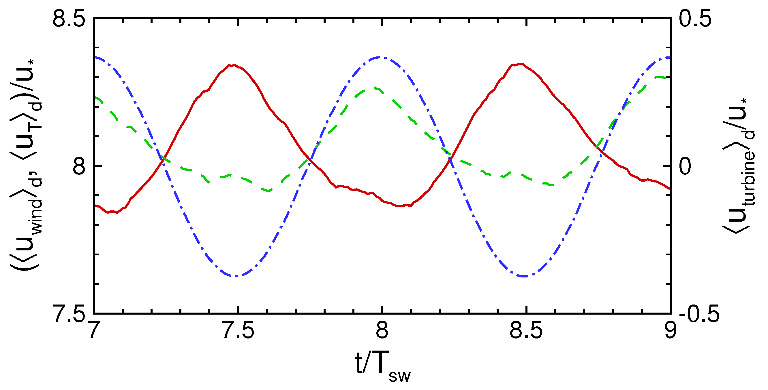
To help understand the change of the phase in oscillating mode, we decomposed disk averaged reference wind velocity , where is the disk averaged incoming wind velocity, and is the disk averaged velocity of the turbine pitch motion, where when the turbine disk flaps toward the downwind direction (e.g., from Phase 4 in Figure 4d to Phase 1 in Figure 4a, and then to Phase 2 in Figure 4b). Figure 10 shows the time series of these three velocities. While is the maximum above the trough (e.g., at in Figure 10), the turbine-rotor disk also flaps toward the downwind direction at its maximum speed. The combined effect results in a reversed phase in with respect to for the pitch-motion magnitude considered in this study. We note that, for other types of floating platforms that have different phase dependence for their floating motions with respect to the swell waves, the resultant oscillation of the turbine power-extraction rate may have swell-correlated oscillation with different magnitude and phase dependence compared to the case considered in this study. Nevertheless, the results reported here illustrate a possible scenario for which turbine pitch motion induces a noticeable effect to the power-extraction rate. Because is directly related to turbine force , the results shown in this study also suggest that it may be important to take into account swell-phase correlated wind-load oscillation together with swell-induced pitch motion when performing structure analysis and applying a control algorithm for offshore floating wind turbines (e.g., References [51,52]).
4. Conclusions
Offshore wind turbines deployed in deep-water regions are usually designed to be installed on floating platforms. Under strong wave and wind forcing conditions, the platform can exhibit considerable oscillating motions that can affect wind-turbine performance and structure dynamics. In this study, we performed numerical experiments and statistical analysis to study the effect of swell-wave-induced turbine pitch motion on the statistics of wind turbulence around the turbine and the wind-power extraction rate. We considered a sea-surface wave field consisting of a background broadband wind-wave field and a strong swell-wave train with wavelength and steepness propagating in the downwind direction. To study the effects of turbine pitch motion on wake turbulence statistics and wind-power extraction, we considered a reference case with fixed wind turbines and a floating-turbine case in which swell-induced turbine pitch motion was considered. Because the motions of the turbine platform can be affected by many factors, such as wind, waves, tides, ocean currents, platform geometry, and mooring system, actual turbine motions in real offshore operational environments are highly complicated. Modeling turbine-platform dynamics with all these factors considered is a comprehensive research topic by itself. For the sake of simplicity for both the simulation and data analysis, in this study we only considered the dominant pitch-motion mode, consisting of a mean pitch angle of 4 degrees due to mean wind forcing, and a swell-correlated pitch with a magnitude of 5 degrees and a phase of degrees relative to the swell-wave phase. The turbine pitch motion is prescribed in the simulation.
To capture the effect of surface waves and turbine pitch motion on wind–turbine interactions, we employed a hybrid numerical model that couples the LES of wind turbulence with the HOSM of sea-surface waves. We focused on using the swell-phase averaging approach to obtain flow statistics that revealed strong swell-phase correlation in turbulence statistics and extracted power density by wind turbines. For both the fixed- and floating-turbine cases considered in this study, the strong swell waves generated apparent swell-correlated variation in turbulence statistics such as phase-averaged wind velocities, velocity variance, and Reynolds stress. Comparison between the fixed- and floating-turbine cases showed that swell-induced turbine pitch motion causes noticeable oscillations of vertical-velocity variance and Reynolds stress, as well as an increase in magnitude for the vertical-velocity variance around the upper edge of the turbine rotor by ∼15%. The periodically occurring high-speed wind above the swell troughs results in swell-correlated oscillation in extracted power density in the fixed-turbine case. With the turbine pitch motion modeled in this study, the phase dependence of on swell waves was shifted by nearly 180 degrees due to the combined effects of swell-induced wind-velocity oscillation, and turbine-rotor-disk velocity due to pitch motion.
Author Contributions
S.X. performed the simulations, analyzed the results, and wrote the first draft of the paper. D.Y. formulated the problem, interpreted the results, and contributed to writing the paper.
Funding
This research was supported by Di Yang’s start-up funds at the University of Houston.
Acknowledgments
The authors acknowledge the use of the Opuntia Cluster and the advanced support from the Core Facility for Advanced Computing and Data Science at the University of Houston to carry out the numerical simulations presented here.
Conflicts of Interest
The authors declare no conflict of interest.
Abbreviations
The following abbreviations are used in this manuscript:
| LES | large-eddy simulation |
| HOSM | high-order spectral method |
| ABL | atmospheric boundary layer |
| SGS | subgrid scale |
| LASD | Lagrangian-averaged scale-dependent |
References
- Wind Vision: A New Era for Wind Power in the United States; Technical Report; U.S. Department of Energy: Washington, DC, USA, 2015. Available online: https://www.energy.gov/eere/wind/wind-vision (accessed on 10 February 2019).
- 20% Wind Energy by 2030: Increasing Wind Energy’s Contribution to U.S. Electricity Supply; Technical Report; U.S. Department of Energy: Washington, DC, USA, 2008.
- Zervos, A.; Kjaer, C. Pure Power: Wind Energy Scenarios up to 2030; Technical Report; European Wind Energy Association: Brussels, Belgium, 2008. [Google Scholar]
- Edson, J.; Crawford, T.; Crescenti, J.; Farrar, T.; Frew, N.; Gerbi, G.; Helmis, C.; Hristov, T.; Khelif, D.; Jessup, A.; et al. The coupled boundary layers and air-sea transfer experiment in low winds. Bull. Am. Meteor. Soc. 2007, 88, 341–356. [Google Scholar] [CrossRef]
- Sullivan, P.P.; McWilliams, J.C. Dynamics of winds and currents coupled to surface waves. Annu. Rev. Fluid Mech. 2010, 42, 19–42. [Google Scholar] [CrossRef]
- Sullivan, P.P.; McWilliams, J.C.; Patton, E.G. Large-eddy simulation of marine atmospheric boundary layers above a spectrum of moving waves. J. Atmos. Sci. 2014, 71, 4001–4027. [Google Scholar] [CrossRef]
- Yang, D.; Meneveau, C.; Shen, L. Large-eddy simulation of offshore wind farm. Phys. Fluids 2014, 26, 025101. [Google Scholar] [CrossRef]
- Sullivan, P.P.; Edson, J.B.; Hristov, T.; McWilliams, J.C. Large-eddy simulations and observations of atmospheric marine boundary layers above nonequilibrium surface waves. J. Atmos. Sci. 2008, 65, 1225–1245. [Google Scholar] [CrossRef]
- Yang, D.; Meneveau, C.; Shen, L. Effect of downwind swells on offshore wind energy harvesting—A large-eddy simulation study. Renew. Energy 2014, 70, 11–23. [Google Scholar] [CrossRef]
- Rockel, S.; Camp, E.; Schmidt, J.; Peinke, J.; Cal, R.B.; Hölling, M. Experimental study on influence of pitch motion on the wake of a floating wind turbine model. Energies 2014, 7, 1954–1985. [Google Scholar] [CrossRef]
- Rockel, S.; Peinke, J.; Hölling, M.; Cal, R.B. Wake to wake interaction of floating wind turbine models in free pitch motion: An eddy viscosity and mixing length approach. Renew. Energy 2016, 85, 666–676. [Google Scholar] [CrossRef]
- Wen, B.; Dong, X.; Tian, X.; Peng, Z.; Zhang, W.; Wei, K. The power performance of an offshore floating wind turbine in platform pitching motion. Energy 2018, 154, 508–521. [Google Scholar] [CrossRef]
- Stenvens, R.J.A.M.; Martínez-Tossas, L.A.; Meneveau, C. Comparison of wind farm large eddy simulations using actuator disk and actuator line models with wind tunnel experiments. Renew. Energy 2018, 116, 470–478. [Google Scholar] [CrossRef]
- Stenvens, R.J.A.M.; Meneveau, C. Flow structure and turbulence in wind farms. Annu. Rev. Fluid Mech. 2017, 49, 311–339. [Google Scholar] [CrossRef]
- Calaf, M.; Meneveau, C.; Meyers, J. Large eddy simulation study of fully developed wind-turbine array boundary layers. Phys. Fluids 2010, 22, 015110. [Google Scholar] [CrossRef] [Green Version]
- Calaf, M.; Parlange, M.; Meneveau, C. Large eddy simulation study of scalar transport in fully developed wind-turbine array boundary layers. Phys. Fluids 2011, 23, 126603. [Google Scholar] [CrossRef] [Green Version]
- Stenvens, R.J.A.M.; Gayme, D.F.; Meneveau, C. Large eddy simulation studies of the effects of alignment and wind farm length. J. Renew. Sustain. Energy 2014, 6, 023105. [Google Scholar] [CrossRef] [Green Version]
- Stenvens, R.J.A.M.; Meneveau, C. Temporal structure of aggregate power fluctuations in large-eddy simulations of extended wind-farms. J. Renew. Sustain. Energy 2014, 6, 043102. [Google Scholar] [CrossRef] [Green Version]
- VerHulst, C.; Meneveau, C. Large eddy simulation study of the kinetic energy entrainment by energetic turbulent flow structures in large wind farms. Phys. Fluids 2014, 26, 025113. [Google Scholar] [CrossRef]
- Yang, X.; Kang, S.; Sotiropoulos, F. Computational study and modeling of turbine spacing effects in infinite aligned wind farms. Phys. Fluids 2012, 24, 115107. [Google Scholar] [CrossRef]
- Yang, X.; Sotiropoulos, F. LES investigation of infinite staggered wind-turbine arrays. J. Phys. Conf. Ser. 2014, 555, 012109. [Google Scholar] [CrossRef] [Green Version]
- Zhang, M.; Arendshorst, M.G.; Stevens, R. Large eddy simulations of the effect of vertical staggering in large wind farms. Wind Energy 2018, 22, 189–204. [Google Scholar] [CrossRef]
- Lyu, P.; Park, S.G.; Shen, L.; Li, H. A coupled wind-wave-turbine solver for offshore wind farm. In Proceedings of the ASME 2018 1st International Offshore Wind Technical Conference, San Francisco, CA, USA, 4–7 November 2018; IOWTC2018-1046. ASME: New York, NY, USA, 2018. [Google Scholar] [CrossRef]
- Dörenkämper, M.; Witha, B.; Steinfeld, G.; Heinemann, D.; Kühn, M. The impact of stable atmospheric boundary layers on wind-turbine wakes within offshore wind farms. J. Wind Eng. Ind. Aerod. 2015, 144, 146–153. [Google Scholar] [CrossRef] [Green Version]
- Allaerts, D.; Meyers, J. Boundary-layer development and gravity waves in conventionally neutral wind farms. J. Fluid Mech. 2017, 814, 95–130. [Google Scholar] [CrossRef] [Green Version]
- Jimenez, A.; Crespo, A.; Migoya, E.; Garcia, J. Advances in large-eddy simulation of a wind turbine wake. J. Phys. Conf. Ser. 2007, 75, 012041. [Google Scholar] [CrossRef] [Green Version]
- Jimenez, A.; Crespo, A.; Migoya, E.; Garcia, J. Large-eddy simulation of spectral coherence in a wind turbine wake. Environ. Res. Lett. 2008, 3, 015004. [Google Scholar] [CrossRef] [Green Version]
- Meyers, J.; Meneveau, C. Large eddy simulation of large wind-turbine arrays in the atmospheric boundary layer. AIAA 2010. [Google Scholar] [CrossRef]
- Naderi, S.; Parvanehmasiha, S.; Torabi, F. Modeling of horizontal axis wind turbine wakes in Horns Rev offshore wind farm using an improved actuator disc model coupled with computational fluid dynamic. Energy Convers. Manag. 2018, 171, 953–968. [Google Scholar] [CrossRef]
- Smagorinsky, J. General circulation experiments with the primitive equations. I. The basic experiment. Mon. Weather Rev. 1963, 91, 99–164. [Google Scholar] [CrossRef]
- Lilly, D.K. The representation of small-scale turbulence in numerical simulation experiments. In Proceedings of the IBM Scientific Computing Symposium on Environmental Science, Boulder, CO, USA, 14–16 November 1966; Goldstein, H.H., Ed.; IBM: Yorktown Heights, NY, USA, 1967; pp. 195–210. [Google Scholar]
- Bou-Zeid, E.; Meneveau, C.; Parlange, M. A scale-dependent Lagrangian dynamic model for large eddy simulation of complex turbulent flows. Phys. Fluids 2005, 17, 025105. [Google Scholar] [CrossRef] [Green Version]
- Wan, F.; Porté-Agel, F.; Stoll, R. Evaluation of dynamic subgrid-scale models in large-eddy simulations of neutral turbulent flow over a two-dimensional sinusoidal hill. Atmos. Environ. 2007, 41, 2719–2728. [Google Scholar] [CrossRef]
- Kumar, V.; Svensson, G.; Holtslag, A.A.M.; Meneveau, C.; Parlange, M. Impact of surface flux formulations and geostrophic forcing on large-eddy simulations of diurnal atmospheric boundary layer flow. J. Appl. Meteorol. Climatol. 2010, 49, 1496–1516. [Google Scholar] [CrossRef]
- Anderson, W.; Meneveau, C. Dynamic roughness model for large-eddy simulation of turbulent flow over multiscale, fractal-like rough surfaces. J. Fluid Mech. 2011, 679, 288–314. [Google Scholar] [CrossRef]
- Yang, D.; Meneveau, C.; Shen, L. Dynamic modelling of sea-surface roughness for large-eddy simulation of wind over ocean wavefield. J. Fluid Mech. 2013, 726, 62–99. [Google Scholar] [CrossRef]
- Yang, D.; Shen, L. Direct-simulation-based study of turbulent flow over various waving boundaries. J. Fluid Mech. 2010, 650, 131–180. [Google Scholar] [CrossRef]
- Yang, D.; Shen, L. Simulation of viscous flows with undulatory boundaries. Part I. Basic solver. J. Comput. Phys. 2011, 230, 5488–5509. [Google Scholar] [CrossRef]
- Dommermuth, D.G.; Yue, D.K.P. A high-order spectral method for the study of nonlinear gravity waves. J. Fluid Mech. 1987, 184, 267–288. [Google Scholar] [CrossRef]
- Mei, C.C.; Stiassnie, M.; Yue, D.K.P. Theory and Applications of Ocean Surface Waves. Part 2: Nonlinear Aspects; World Scientific: Singapore, 2015. [Google Scholar] [CrossRef]
- Alam, M.-R.; Liu, Y.; Yue, D.K.P. Oblique sub- and super-harmonic Bragg resonance of surface waves by bottom ripples. J. Fluid Mech. 2010, 643, 437–447. [Google Scholar] [CrossRef]
- Zakharov, V.E. Stability of periodic waves of finite amplitude on the surface of a deep fluid. J. Appl. Mech. Tech. Phys. 1968, 2, 190–194. [Google Scholar] [CrossRef]
- Hasselmann, K.; Barnett, T.P.; Bouws, E.; Carlson, H.; Cartwright, D.E.; Enke, K.; Ewing, J.A.; Gienapp, H.; Hasselmann, D.E.; Kruseman, P.; et al. Measurements of wind-wave growth and swell decay during the Joint North Sea Wave Project (JONSWAP). Dtsch. Hydrogr. Z. Suppl. 1973, 8, N12. [Google Scholar]
- Wayman, E.N.; Sclavounos, P.D.; Butterfield, S.; Jonkman, J.; Musial, W. Coupled Dynamic Modeling of Floating Wind Turbine Systems; National Renewable Energy Laboratory: Golden, CO, USA, 2006.
- Roddier, D.; Cermelli, C.; Aubault, A.; Weinstein, A. WindFloat: A floating foundation for offshore wind turbines. J. Renew. Sustain. Energy 2010, 2, 033104. [Google Scholar] [CrossRef]
- Jonkman, J.; Matha, D. A Quantitative Comparison of the Responses of Three Floating Platforms; National Renewable Energy Laboratory: Golden, CO, USA, 2010.
- Shoele, K.; Prowell, I.; Zhu, Q.; Elgamal, A. Dynamic and structural modeling of a floating wind turbine. Int. J. Offshore Polar 2011, 21, 155–160. [Google Scholar]
- Li, Y.; Tang, Y.; Zhu, Q.; Liu, L. Study on dynamic response of floating offshore wind turbine based on stretching-bending-torsion coupled nonlinear mooring loads. Eng. Mech. 2018, 35, 229–239. [Google Scholar] [CrossRef]
- Li, Y.; Liu, L.; Zhu, Q.; Guo, Y.; Hu, Z.; Tang, Y. Influence of vortex induced loads on the motion of SPAR-Type wind turbine: A coupled aero-hydro-vortex-mooring investigation. J. Offshore Mech. Arct. Eng. 2018, 140, 051903. [Google Scholar] [CrossRef]
- Barrera, C.; Losada, I.J.; Guanche, R.; Johanning, L. The influence of wave parameter definition over floating wind platform mooring systems under severe sea states. Ocean Eng. 2019, 172, 105–126. [Google Scholar] [CrossRef]
- Lemmer, F.; Schlipf, D.; Cheng, P.W. Control design methods for floating wind turbines for optimal disturbance rejection. J. Phys. Conf. Ser. 2016, 753, 092006. [Google Scholar] [CrossRef] [Green Version]
- Kim, K.; Kim, H.; Lee, J.; Kim, S.; Paek, I. Design and performance analysis of control algorithm for a floating wind turbine on a large semi-submersible platform. J. Phys. Conf. Ser. 2016, 753, 092017. [Google Scholar] [CrossRef] [Green Version]
Figure 1.
Illustration of three-dimensional instantaneous wind- and swell-wave fields in a fully developed offshore-wind-turbine array boundary layer. Contours of instantaneous streamwise wind velocity are plotted on the vertical plane across the center of the third column of turbines in the simulation domain. The turbine rotor disks are illustrated by the black circular disks representing where actuator-disk model forces are applied. The turbine towers and nacelles (shown in gray color) are also plotted only for illustration purposes, and their effects were not considered in the simulations.

Figure 2.
Illustration of turbine pitch motion caused by swell waves: (a) turbine at its maximum downwind pitch position when swell’s forward slope arrives and (b) turbine at its maximum upwind pitch position when swell’s backward slope arrives.
Figure 2.
Illustration of turbine pitch motion caused by swell waves: (a) turbine at its maximum downwind pitch position when swell’s forward slope arrives and (b) turbine at its maximum upwind pitch position when swell’s backward slope arrives.
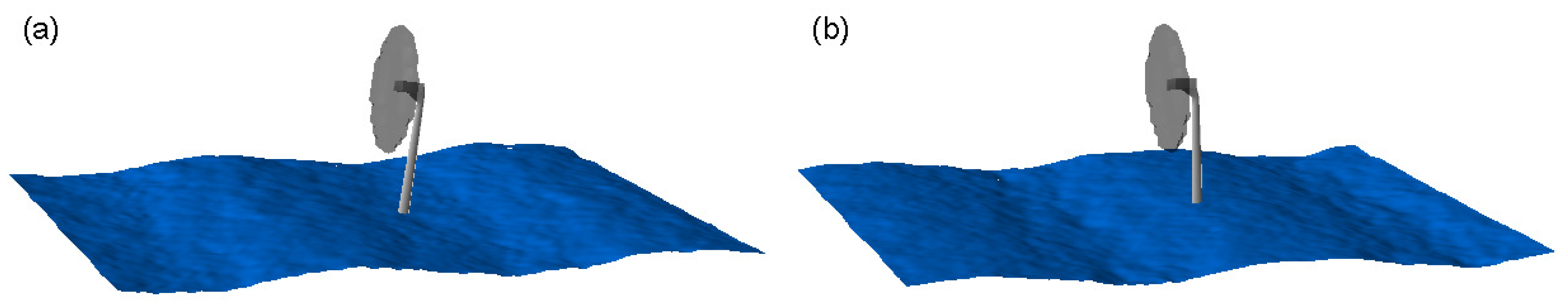
Figure 3.
Statistics of turbulent wind flows for the fixed-turbine case. Statistics were obtained using the swell-phase average approach. Statistics for Phase 2 (when the forward slope of the swell reaches the turbine) are plotted: (a) streamwise velocity ; (b) Reynolds stress ; (c) streamwise velocity variance ; and (d) vertical velocity variance . Statistical quantities were normalized using wind-friction velocity . The location of the turbine-rotor disk is indicated by the thick black line.
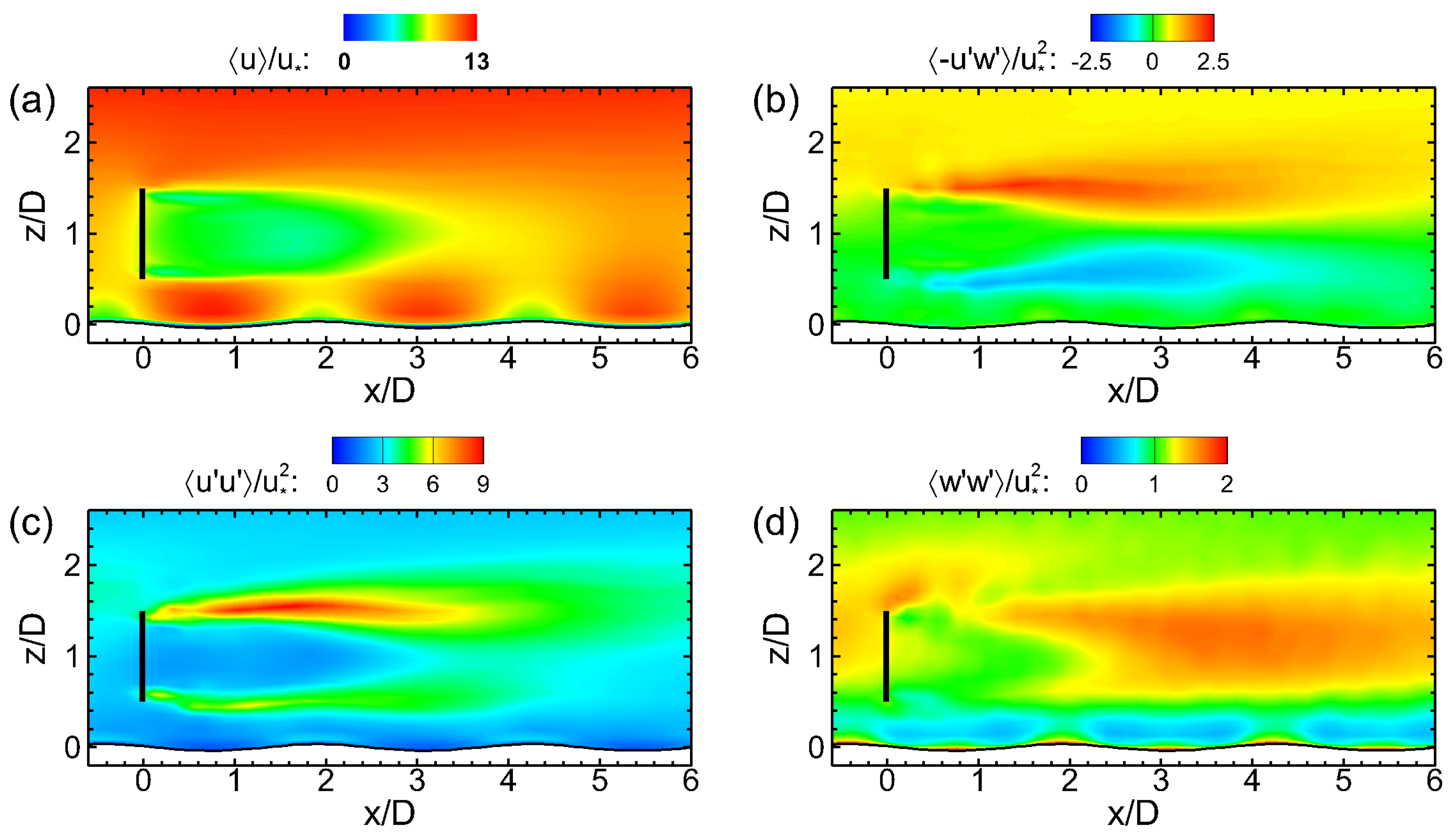
Figure 4.
Swell-phase averaged streamwise wind velocity at four representative swell phases for pitching-turbine case: (a) trough (Phase 1); (b) forward slope (Phase 2); (c) crest (Phase 3); and (d) backward slope (Phase 4). Turbine-rotor-disk location indicated by thick black line.
Figure 4.
Swell-phase averaged streamwise wind velocity at four representative swell phases for pitching-turbine case: (a) trough (Phase 1); (b) forward slope (Phase 2); (c) crest (Phase 3); and (d) backward slope (Phase 4). Turbine-rotor-disk location indicated by thick black line.

Figure 5.
Swell-phase averaged vertical wind velocity at four representative swell phases for pitching-turbine case: (a) trough (Phase 1); (b) forward slope (Phase 2); (c) crest (Phase 3); and (d) backward slope (Phase 4). Turbine-rotor-disk location indicated by thick black line.
Figure 5.
Swell-phase averaged vertical wind velocity at four representative swell phases for pitching-turbine case: (a) trough (Phase 1); (b) forward slope (Phase 2); (c) crest (Phase 3); and (d) backward slope (Phase 4). Turbine-rotor-disk location indicated by thick black line.
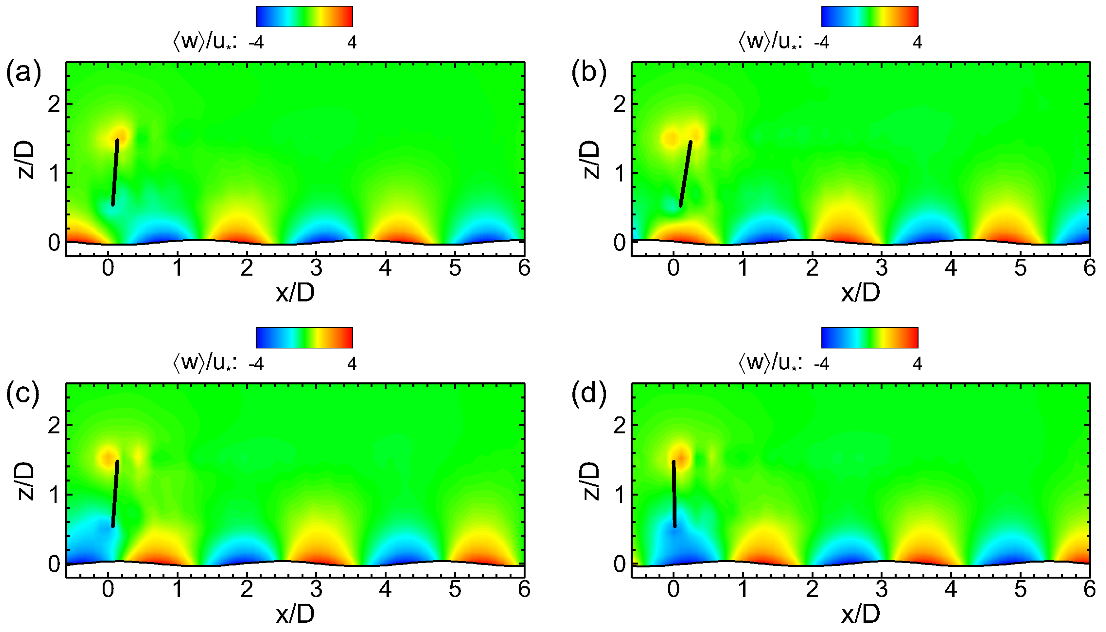
Figure 6.
Swell-phase averaged streamwise wind-velocity variance at four representative swell phases for pitching-turbine case: (a) trough (Phase 1); (b) forward slope (Phase 2); (c) crest (Phase 3); and (d) backward slope (Phase 4). Turbine-rotor-disk location indicated by thick black line.
Figure 6.
Swell-phase averaged streamwise wind-velocity variance at four representative swell phases for pitching-turbine case: (a) trough (Phase 1); (b) forward slope (Phase 2); (c) crest (Phase 3); and (d) backward slope (Phase 4). Turbine-rotor-disk location indicated by thick black line.

Figure 7.
Swell-phase averaged vertical wind-velocity variance at four representative swell phases for pitching-turbine case: (a) trough (Phase 1); (b) forward slope (Phase 2); (c) crest (Phase 3); and (d) backward slope (Phase 4). Turbine-rotor-disk location indicated by thick black line.
Figure 7.
Swell-phase averaged vertical wind-velocity variance at four representative swell phases for pitching-turbine case: (a) trough (Phase 1); (b) forward slope (Phase 2); (c) crest (Phase 3); and (d) backward slope (Phase 4). Turbine-rotor-disk location indicated by thick black line.
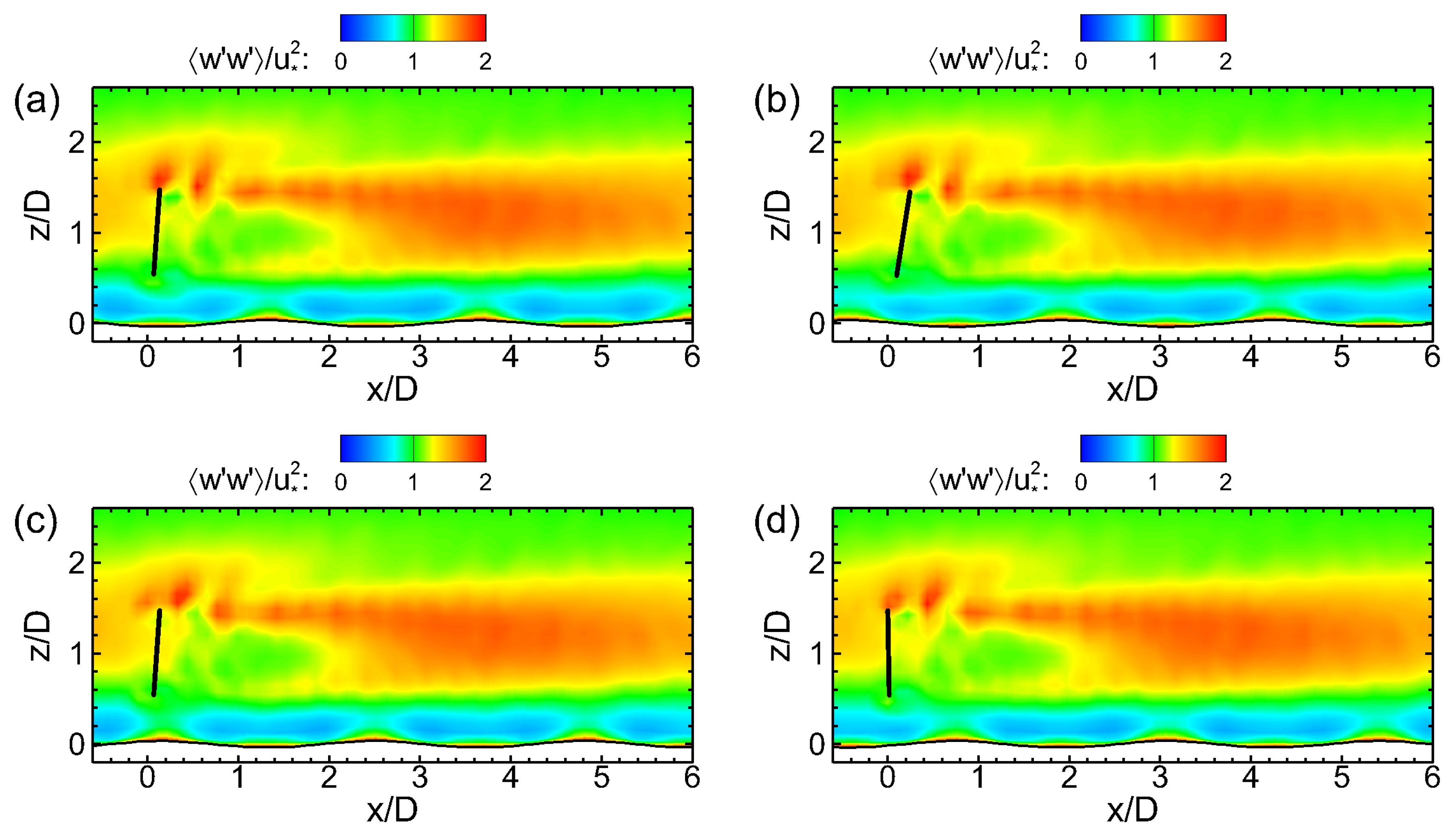
Figure 8.
Swell-phase averaged Reynolds stress at four representative swell phases for pitching-turbine case: (a) trough (Phase 1); (b) forward slope (Phase 2); (c) crest (Phase 3); and (d) backward slope (Phase 4). Turbine-rotor-disk location indicated by thick black line.
Figure 8.
Swell-phase averaged Reynolds stress at four representative swell phases for pitching-turbine case: (a) trough (Phase 1); (b) forward slope (Phase 2); (c) crest (Phase 3); and (d) backward slope (Phase 4). Turbine-rotor-disk location indicated by thick black line.

Figure 9.
Time series of averaged extracted power density of an offshore wind farm for a (a) fixed turbine and (b) floating turbine in swell-wave condition. Power density is normalized by wind-friction velocity , and time t is normalized by swell-wave period . The solid line is for and dashed line indicates the swell phase. For illustration purposes, the amplitude of the swell was not plotted to scale.

Figure 10.
Time series of turbine-rotor-disk averaged velocity components for the floating-turbine case. Here, is the averaged incoming wind velocity (dashed line), is the turbine rotor velocity caused by the swell-induced pitch motion (dash-dot line), and (solid line). Values for and are shown on the vertical axis plotted on the left side (ranging from to , and values for are shown on the vertical axis plotted on the right side (ranging from to ).
© 2019 by the authors. Licensee MDPI, Basel, Switzerland. This article is an open access article distributed under the terms and conditions of the Creative Commons Attribution (CC BY) license (http://creativecommons.org/licenses/by/4.0/).
Share and Cite
MDPI and ACS Style
Xiao, S.; Yang, D. Large-Eddy Simulation-Based Study of Effect of Swell-Induced Pitch Motion on Wake-Flow Statistics and Power Extraction of Offshore Wind Turbines. Energies 2019, 12, 1246. https://doi.org/10.3390/en12071246
AMA Style
Xiao S, Yang D. Large-Eddy Simulation-Based Study of Effect of Swell-Induced Pitch Motion on Wake-Flow Statistics and Power Extraction of Offshore Wind Turbines. Energies. 2019; 12(7):1246. https://doi.org/10.3390/en12071246
Chicago/Turabian StyleXiao, Shuolin, and Di Yang. 2019. "Large-Eddy Simulation-Based Study of Effect of Swell-Induced Pitch Motion on Wake-Flow Statistics and Power Extraction of Offshore Wind Turbines" Energies 12, no. 7: 1246. https://doi.org/10.3390/en12071246
Note that from the first issue of 2016, this journal uses article numbers instead of page numbers. See further details here.