Accuracy and Reliability of Switching Transients Measurement with Open-Air Capacitive Sensors

Abstract

Contactless capacitive (open-air) sensors are applied to monitor overvoltages near overhead line terminations at a substation or at the transition from underground cables to overhead lines. It is shown that these sensors, applied in a differentiating/integrating measuring concept, can result in excellent characteristics in terms of electromagnetic compatibility. The inherent cross-coupling from open-air sensors to other phases is dealt with. The paper describes a method to calibrate the sensor to line coupling matrix based on assumed 50 Hz symmetric phase voltages and in particular focuses on uncertainty analysis of assumptions made. Network simulation shows that predicted maximum overvoltages agree within typically 7% compared to reconstructed values from measurement, also with significant cross-coupling. Transient voltages from energization of an (extra-)high voltage connection can cause large and steep rising ground currents near the line terminations. Comparison with results obtained by a capacitive divider confirms the intrinsic capability in interference rejection by the differentiating/integrating measurement methodology.

1. Introduction

Knowledge on actual overvoltages from transients in electrical transmission systems can be very helpful to estimate optimal measures for overvoltage protection, to understand the background of problems (if any) and/or to estimate related degradation of electrical insulation. Such transients arise e.g., from line energization and can cover a wide frequency spectrum [1]. The installation of equipment such as (R) C-dividers capable to capture high-frequency signals is costly, leaves a relatively big footprint and should be planned ahead. Dividers can also be prone to EMC (electromagnetic compatibility) disturbance [2], e.g., arising from ground currents upon a switching event. A non-invasive, cost-efficient, easy to (re-)install and EMC-proof measurement system would therefore be appealing to occasionally perform voltage monitoring.

This paper describes applications based on open-air capacitive sensors as part of a D/I (differentiating/integrating) measurement concept. The signal at the measurement cable end, characteristically terminated with 50 Ω, is basically the time-derivative of the phase-voltage as picked up with the open-air capacitive sensors. These sensors can be mounted in a short time without adaptation to the EHV (extra-high voltage) system. In other words, it is a non-invasive measuring system. The original waveform is restored by means of an analogue integrator. One of the earlier papers describing the method for application on high-voltage measurement is reference [3]. As the sensors basically consist of metal plates which form capacitances to high-voltage conductors nearby, the requirements related to costs, installation effort and being non-invasive are fulfilled. A drawback of the method relates to the prior unknown coupling strengths of open-air sensors and the limited selectivity as they couple to any phase conductor in the vicinity. A matrix containing all couplings between sensors and phases needs to be established to entangle the cross-coupling.

A number of open-air sensor applications with solutions for the selectivity problem can be found in literature. In [4], line energization was studied. Decoupling could be achieved since different phases had distinct contact moments. This allowed to determine the responses of the sensors upon the three distinct energization moments. Each phase energization provided three sensor responses, enabling to establish the complete coupling matrix. In [5] the capacitive sensors were inside a GIS (gas insulated system) and in prior tests the phases could be energized separately. A harmonics study was published in [6] where the sensors were positioned halfway between two overhead line pylons. The capacitances were derived from equations for cylindrical line conductors above perfect conductive earth. Unknowns in distances (e.g., line heights) could be resolved by assuming symmetric power frequency voltages on the overhead lines and fitting the measured and calculated waveforms. For the transient overvoltage study in [7], a similar approach was taken. However, the sensors were placed near the terminations for high sensitivity. Due to the complex termination design, analytical field calculation was not possible, leaving the coupling matrix not fully determined. It was shown that with a few assumptions based on symmetry in the configuration the reconstruction could be realized.

This paper develops a methodology to analyse the consequence of uncertainties in the assumptions made to reconstruct the phase voltages. Section 2 briefly describes the methodology. Confidence bounds are needed to judge the accuracy of network simulations, which are implemented in PSCAD [8]. References [7] and [9] provide information on the modelled network detail and extension, respectively. In Section 3.1, these simulations are compared with measurements in relation to the experimental uncertainty. In [2] the merits of the D/I method in terms of EMC immunity are discussed. To verify the claims, simultaneous measurement of switching transients by the D/I system and a high voltage divider is performed. The reliability of the recordings from both systems is compared in Section 3.2. Section 4 reflects on the results in terms of accuracy as well as reliability and Section 5 concludes with situations for which D/I measurement is particularly of interest.

2. Measurement Analysis and Uncertainty

Measured sensor signals u_i relate to the phase voltages U_j according to a coupling matrix M: u=MU. Reconstruction of the phase voltages from recorded signals can be achieved by inverting this relation. The matrix elements M_ij are obtained by selecting the part from the recorded signals containing only the power frequency waveform (with angular frequency ω₀). Sinusoidal fits u_pf,i are made and related with an assumed base of symmetric (per unit) phase voltages, i.e., equal amplitudes and 120° phase angle differences:

$$\left(\begin{array}{c}{u}_{pf,1}\left(t;{\phi }_0\right)\\ u_{pf,2}\left(t;{\phi }_0\right)\\ u_{pf,3}\left(t;{\phi }_0\right)\end{array}\right)=\left(\begin{array}{ccc}{M}_{11}& M_{12}& M_{13}\\ M_{21}& M_{22}& M_{23}\\ M_{31}& M_{32}& M_{33}\end{array}\right)\left(\begin{array}{c}\cos \left({\omega }_{0}t+⅔\mathsf{\pi }\right)\\ \cos \left({\omega }_{0}t\right)\\ \cos \left({\omega }_{0}t-⅔\mathsf{\pi }\right)\end{array}\right)$$

(1)

$$\mathrm{with}{u}_{pf,i}\left(t;{\phi }_0\right)=a_i\cos \left({\omega }_{0}t+{\phi }_0\right)+b_i\sin \left({\omega }_{0}t+{\phi }_0\right)$$

The reference time t = 0 in (1) corresponds with the central phase reaching its maximum value. If the trigger moment of the measurement device is not synchronized with (one of) the phase voltages, it can be implemented as a phase shift ϕ₀. This additional unknown can be omitted by having the measurement time base related to a simultaneous recording of the phase voltage information, e.g., from a voltage transformer (synchronized), or it can be obtained from the measured waveforms themselves (unsynchronized). As (1) relates sinusoidal waves of a single frequency, each row equation determines only two parameters and the set of three equations is underdetermined. With ten unknowns (for unsynchronized measurements) and six fitted parameters also other sources of information must be employed. Reduction of the number of independent components M_ij can be achieved by neglecting components when these are very small, or by having a symmetric positioning of sensors with respect to the phase conductors meaning that various matrix components are equal [7,10]. Also parameter estimates can be made and their uncertainties can be retrieved, e.g., from comparison with numerical electrostatic field simulations on the system. Which assumptions are to be made and what the effects will be on the uncertainty margins are specific for the configuration at the measurement site. Measurements of energization transients are obtained from a double circuit 380 kV line-cable-line connection [7]. More specifically, measurements were taken at the underground cable to overhead line transition points (at both cable ends) and near an overhead line termination at one of the substations.

Uncertainty analysis concerns the determination on how input margins propagate into end result deviations according the designed measurement chain. In addition, reliability of the measurement can be impeded when also signal coupling along an unintended route takes place. This can be a serious problem when recording switching transients in (E)HV networks. Line energization causes steep switching fronts which, in particular at an overhead line to underground cable transition, may induce ground currents. These currents may partly find their way along the metallic screens of the measurement cables. Depending on the measurement system design and layout, this can disturb signal recordings.

In Figure 1 the configuration for a D/I system is compared to a capacitive divider configuration. The D/I sensor consisted of two 30 × 30 cm² plates, with the top plate sensing the phase voltages (C_HV = 0.1–1 pF) and the bottom plate connected to earth. For the D/I method, the capacitance between the plates is relatively low (here C_E ≈ 300 pF). The measurement cable is characteristically terminated and its impedance R_m is far lower than |Z_E| = 1/(ωC_E). Up to the cut-off frequency, 1/(2πR_mC_E), the time derivative U’(t) arises at the cable end. The signal waveform is restored by integration with an integrator time constant, τ_int, depending on the integrator design. The active/passive integrator employed for the measurements is described in [11]. The over-all system response U(t) is given by:

$$\begin{array}{c}U\left(t\right)=\frac{1}{{\tau }_{int}}\int U^{\prime }\left(t\right)\mathrm{d}t\mathrm{where}{U}^{\prime }\left(t\right)={\tau }_{dif}\frac{\mathrm{d}{U}_{HV}\left(t\right)}{\mathrm{d}t}\\ {\tau }_{dif}=R_m{C}_{HV}\end{array}$$

(2)

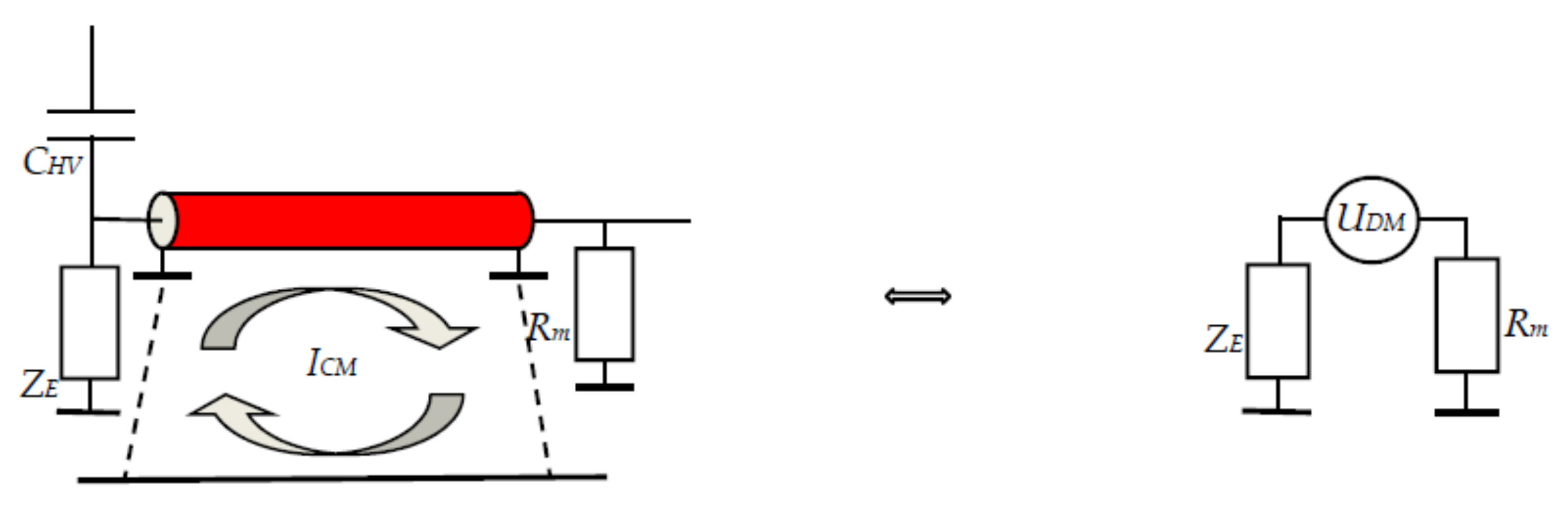
For a divider topology the situation is reversed and the impedance R_m is large compared to |Z_E| in order not to load the low voltage branch of the divider. This difference has repercussions on EMC aspects from ground currents as demonstrated in Figure 2. A part of the ground current will find its way along the measurement cable screens through magnetic induction. This common mode current I_CM will cause a differential mode voltage U_DM which adds to the intended signal. Its value depends on the quality of the measurement cable, which can be expressed as its transfer impedance Z_t [12]:

$$U_{DM}=I_{CM}·Z_t$$

(3)

The fraction of U_DM arising at the receiving end of the cable is a division over the impedances at both ends as shown in the right side of Figure 2. For the D/I concept this is rather a small fraction, whereas for a divider it is the major part. In addition, the integration step in the D/I system reduces high frequency interference, which may have entered the measurement cable. Results will be presented comparing the D/I approach with results from pre-installed dividers near underground power cables at their transition points to overhead lines.

3. Results

The challenge with open-air sensors is to entangle the cross-coupling. The approach advocated in this paper is to employ only the stationary power frequency component from symmetric phase voltages. This requires a minimal installation effort to set up the measurement system, which can be done in typically one to one and a half hour. The option to sequentially inject a signal in each phase and determine the responses as in [5] would provide sufficient information to derive the complete coupling matrix, but it takes time and requires extensive safety precautions. Using the first arriving travelling wave fronts as in [4] assumes that these remain sufficiently clear and recognizable after travelling along the lines and cables. The cross-bonding applied along the underground power cable system modifies the waveform further and therefore such a method is mainly feasible when measurements are conducted near the substation where the switching activities take place.

Different causes for uncertainty are analysed in [10]. The measurement accuracy was checked by determining the variation of the coupling matrix throughout a measurement session at a single location. As the sensors remain at fixed positions, variations are related to noise, stability of the D/I measurement system (in particular the active integrator part) and fitting technique. The overall variation remained within 2%. Deviation from assumed symmetric phase voltages will translate into similar magnitude variations in the recorded signals. However, it was shown that in terms of per unit values, i.e., the percentage of the overvoltage related to the amplitude of the power frequency component, such deviation is negligible. The uncertainty analysed in Section 3.1 concerns the assumptions made in order to reduce the number of independent matrix components in (1). Furthermore, imprecise sensor positioning or metal structures in the vicinity may contribute to deviations from model assumptions.

Section 3.1 details the methodology to establish the coupling matrix for two distinct measurement locations. Section 3.2 elaborates on comparison with system simulation and comparison between D/I and divider measurement.

3.1. Accuracy of Decoupling Procedure

The left side of each row equation in (1) is fitted with the steady state power frequency part of the recorded signal. A single frequency sinusoidal function is determined by two parameters, meaning each row equation in (1) is underdetermined. Since the phase voltages are symmetric, with their sum equal to zero, a constant Δ_i added to each component in row i (i = 1, …, 3) will result in the same function and therefore will still satisfy the fitted relation on the left hand side: all components within a row are determined up to the same constant. Usually, the far end couplings (M₁₃ and M₃₁) are relatively small with respect to the direct couplings (M_ii). Neglecting these or assigning an estimated (small) value will therefore only have a minor effect. For the middle row in (1), in case of a reflection symmetric configuration, the additive value is principally undetermined. However, deviations from symmetry should be accountable to provide for a margin in ϕ₀. Therefore, a fourth uncertainty, Δ₀, is introduced. The coupling matrix with four uncertainties related to the same number of lacking parameter information after fitting can be formulated as:

$$M=\left(\begin{array}{ccc}{M}_{11}& M_{12}& M_{13}\\ M_{21}& M_{22}& M_{23}\\ M_{31}& M_{32}& M_{33}\end{array}\right)\pm \left(\begin{array}{ccc}{\Delta }_1& {\Delta }_1& {\Delta }_1\\ {\Delta }_2-½{\Delta }_0& {\Delta }_2& {\Delta }_2+½{\Delta }_0\\ {\Delta }_3& {\Delta }_3& {\Delta }_3\end{array}\right)$$

(4)

For distinct locations, site specific assumptions will be made with confidence intervals and the consequence on the reconstructed transient waveforms is determined as discussed below.

The components in coupling matrix M_ij in (4) can be re-ordered such that they constitute a linear set of nine parameters indicated as $x_{k=3\left(i-1\right)+j}=M_{ij}$. For these parameters the error matrix E_x needs to be established, which contains all variances and covariances:

$$E_{x,kl}=\langle \mathsf{\Delta }{x}_k\mathsf{\Delta }{x}_l\rangle =\langle {\left(x-\overline{x}\right)}_k{\left(x-\overline{x}\right)}_l\rangle$$

(5)

To this end, normal distributions are assigned to the four uncertainties in (4) and 1000 simulations are made to evaluate (5). The reconstructed phase voltages can be found by inverting matrix M and applying it to recorded waveforms containing the transient events. The components of the inverted coupling matrix M⁻¹ can be arranged in a linear set $y_{l=3\left(i-1\right)+j}=M_{ij}^{-1}$ as well, and its error matrix E_y can be evaluated according [13,14]:

$$E_y=O_{\mathbf{1}}{E}_x{O}_{\mathbf{1}}^T\mathrm{with}{O}_{1,lk}=\frac{\partial y_l}{\partial x_k}$$

(6)

The matrix O₁ represents a linearization of how component y_l of the inverted matrix depends on a variation in the value x_k of the original coupling matrix. Its calculation can conveniently be implemented by slightly varying numerically each coupling matrix component M_ij separately. Next, the phase voltage waveforms are reconstructed by matrix multiplication for each sample in the measurement recordings. The propagation of the error is described by means of matrix O₂ which provides information on how each of the three reconstructed phase voltages varies upon variation in each of the inverted matrix components. The reconstructed phase waveforms are evaluated with [13,14]:

$$E_U=O_{\mathbf{2}}{E}_y{O}_{\mathbf{2}}^T\mathrm{with}{O}_{2,jl}=\frac{\partial U_j}{\partial y_l}\Rightarrow$$

$$O_{\mathbf{2}}=\left(\begin{array}{ccc}\begin{array}{ccc}{u}_1& u_2& u_3\\ 0& 0& 0\\ 0& 0& 0\end{array}& \begin{array}{ccc}0& 0& 0\\ u_1& u_2& u_3\\ 0& 0& 0\end{array}& \begin{array}{ccc}0& 0& 0\\ 0& 0& 0\\ u_1& u_2& u_3\end{array}\end{array}\right)$$

(7)

This equation is applied for each measured sample point. The square roots of the diagonal components in E_U provide the standard deviations for each phase (per sample point). Adding and subtracting the deviations provide the confidence intervals of the reconstructed waveforms.

3.1.1. Substation

The configuration with a line ending at a GIS substation is depicted in Figure 3a. The chosen sensor positioning leaves a reflection symmetric configuration. This leads to equal coupling of the central sensor to the outer phase voltages. Similarly, the coupling of the outer sensors to the central phase conductors are equal. A fundamental problem, as mentioned above, relates to the fact that from calibrating by means of symmetric phase voltages it is impossible to distinguish the contribution of the coupling to the central sensor by the central phase from the combined coupling with the outer phases. An estimate is needed including sufficient margin to accommodate for its uncertainty [10]:

$$M=\left(\begin{array}{ccc}{M}_1& M_4& f_0{M}_4\\ M_5-½{\Delta }_0& M_2& M_5+½{\Delta }_0\\ f_0{M}_6& M_6& M_3\end{array}\right)\mathrm{with}{M}_5=½\left(M_4+M_6\right)$$

(8)

The main couplings in Figure 3a, diagonal elements in (8), are taken independent. Although they are expected to be similar, the effect of imprecise sensor positioning on the main coupling can be accounted for. The couplings of the side sensors to the middle phase are taken independent as well. The coupling to the phase furthest away is roughly estimated to be about 30% of the neighbour couplings M₄ and M₆ with an uncertainty of 50% (i.e., f₀ = 0.30 ± 0.15, so between a fraction of 0.15 to 0.45 of the value of M₄ and M₆). The estimate is based on the distance ratio sensor line, which was just over a factor two. As the sensor couples to a relatively short line, its sensed electric flux is expected to decay between 1/r (long line) and 1/r² (point source). The chosen range with uncertainty covers both extremes. Electrostatic field simulation [7] provided a value of 40%. For M₅ an average value of M₄ and M₆ is taken as the distances are similar. With Δ₂ an uncertainty is assigned in this assumption of 50% of its value (Δ₂ = ½M₅). As precise positioning of the sensor in front of the central phase could relatively easy be judged, the value of Δ₀ was taken 20% of M₅ (Δ₀ = ⅕M₅).

Solving (1) with (8) as coupling matrix results in the following set of equations:

$$\begin{array}{c}{M}_4=\frac{⅓\sqrt{3}\left(a_1\sin {\phi }_0-b_1\cos {\phi }_0\right)+\left(a_1\cos {\phi }_0+b_1\sin {\phi }_0\right)}{1-f_0}{M}_1=⅔\sqrt{3}\left(a_1\sin {\phi }_0-b_1\cos {\phi }_0\right)+f_0{M}_4\\ M_6=\frac{⅓\sqrt{3}\left(-a_3\sin {\phi }_0+b_3\cos {\phi }_0\right)+\left(a_3\cos {\phi }_0+b_3\sin {\phi }_0\right)}{1-f_0}{M}_3=⅔\sqrt{3}\left(-a_3\sin {\phi }_0+b_3\cos {\phi }_0\right)+f_0{M}_6\\ M_2=½\left(M_4+M_6\right)+\left(a_2\cos {\phi }_0+b_2\sin {\phi }_0\right)\end{array}$$

(9)

$$⅔\sqrt{3}\left(-a_2\sin {\phi }_0+b_2\cos {\phi }_0\right)-{\Delta }_0=0$$

(10)

The parameters a_i and b_i are obtained from fitting sinusoidal functions to the last five cycles in the recordings as shown in Figure 4a (left). Equation (10) is solved numerically in ϕ₀ and subsequently all matrix components M_i can be calculated. The solution depends on the stochastic variable Δ₀. The other stochastic variables do not affect the solution of (1) and their effect on the coupling matrix elements can be added afterwards.

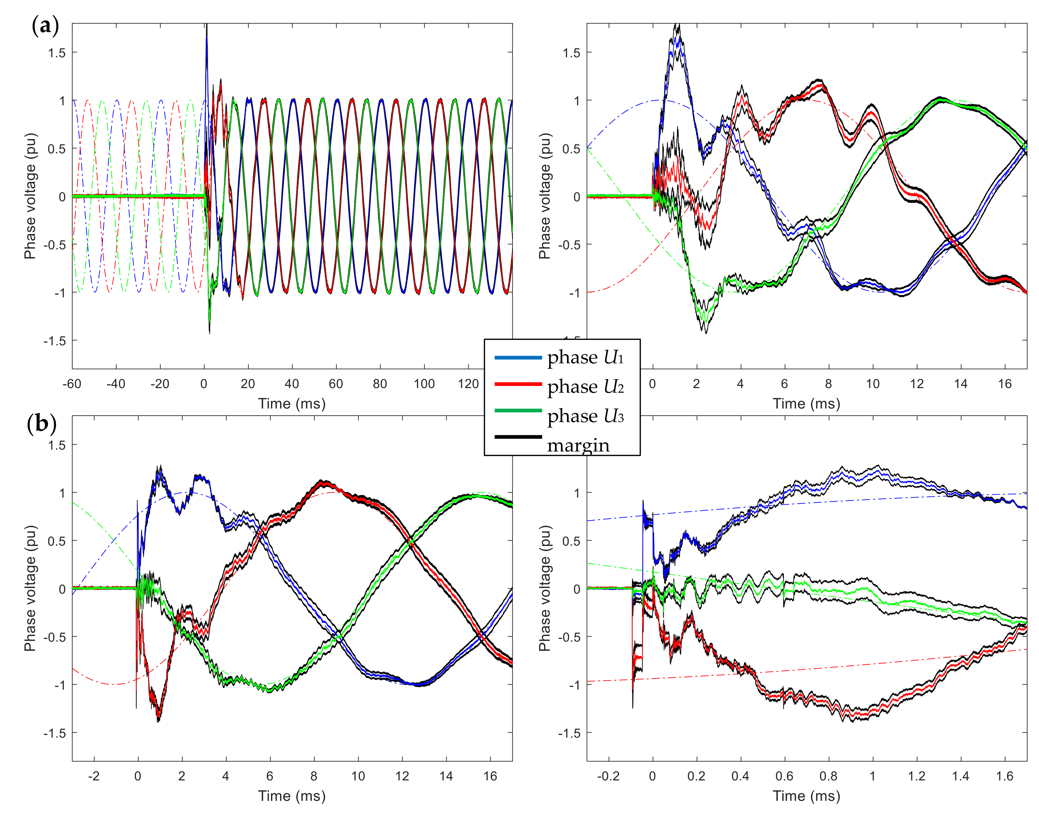
Figure 4 shows the results upon line energization from the far end of the connection and from the substation where the measurements are taken. The black lines indicate one standard deviation confidence margin and the dash-dotted lines are extrapolated steady state phase voltages. The complete waveform in Figure 4a includes the recording of the steady state power frequency established after the switching transient. The last five cycles are employed for determining the coupling matrix. The zoomed figure shows that within the confidence bounds the overvoltage magnitude remains clearly below 2 pu. The switching event in Figure 4b contains steep transients as energization takes place near the measurement location. The zoomed waveform indicates that these relate to travelling waves, which reflect on the line to cable transition point at 6.8 km distance. Also here no serious overvoltages were observed.

3.1.2. Transition Point

The configuration at a transition point is depicted in Figure 3b. Each overhead line is connected with two underground cables to match transmission capacity. The sensors are placed in between the cable terminations belonging to the same phase. The huge terminations provide shielding from coupling to the other phases. Therefore, the far end couplings (u₁ to U₃ and u₃ to U₁) are small and could in principle be neglected. The configuration also suggests that the couplings of sensor u_i to phase U_i+1 have similar magnitudes as is the case for the couplings of sensor u_i+1 to phase U_i (i = 1, 2):

$$M=\left(\begin{array}{ccc}{M}_1& M_4& f_0{M}_1\\ M_5-½{\Delta }_0& M_2& M_4+½{\Delta }_0\\ f_0{M}_3& M_5& M_3\end{array}\right)$$

(11)

From Figure 3b the main couplings, diagonal elements in (11), are expected to be close, but in case of imprecise sensor positioning deviations can be accounted for by allowing independent values. Symmetry in the configuration allows to define only two distinct parameters for coupling of a sensor to a neighbouring phase. A further assumption relates to the far end couplings, which are minor contributions due to the shielding by the terminations. Electrostatic field analysis provided an estimate of 2% [7], which is implemented with an uncertainty margin of 50%: Δ₁ = Δ₃ = ¼f₀(M₁+M₃) with f₀=0.02. In the second row the uncertainty is taken 50% of the average value of the neighbour couplings, Δ₂=¼(M₄+M₅). The additional uncertainty Δ₀, as the measurement equipment was not synchronized with the phase voltages, is taken equal to Δ₂ and accounts for the uncertainty caused by ϕ₀. This reduces M to five independent components.

Solving (1) with (11) results in

$$\begin{array}{c}{M}_1=\frac{⅔\sqrt{3}\left(a_1\sin {\phi }_0-b_1\cos {\phi }_0\right)}{1-f_0}{M}_4=½M_1\left(1+f_0\right)+\left(a_1\cos {\phi }_0+b_1\sin {\phi }_0\right)\\ M_3=\frac{⅔\sqrt{3}\left(-a_3\sin {\phi }_0+b_3\cos {\phi }_0\right)}{1-f_0}{M}_5=½M_3\left(1+f_0\right)+\left(a_3\cos {\phi }_0+b_3\sin {\phi }_0\right)\\ M_2=½\left(M_4+M_5\right)+\left(a_2\cos {\phi }_0+b_2\sin {\phi }_0\right)\end{array}$$

(12)

$$⅔\sqrt{3}\left(-a_2\sin {\phi }_0+b_2\cos {\phi }_0\right)-M_4+M_5-{\Delta }_0=0$$

(13)

Equations (12) and (13) can be solved numerically after fitting the power frequency parts of the recorded waveforms.

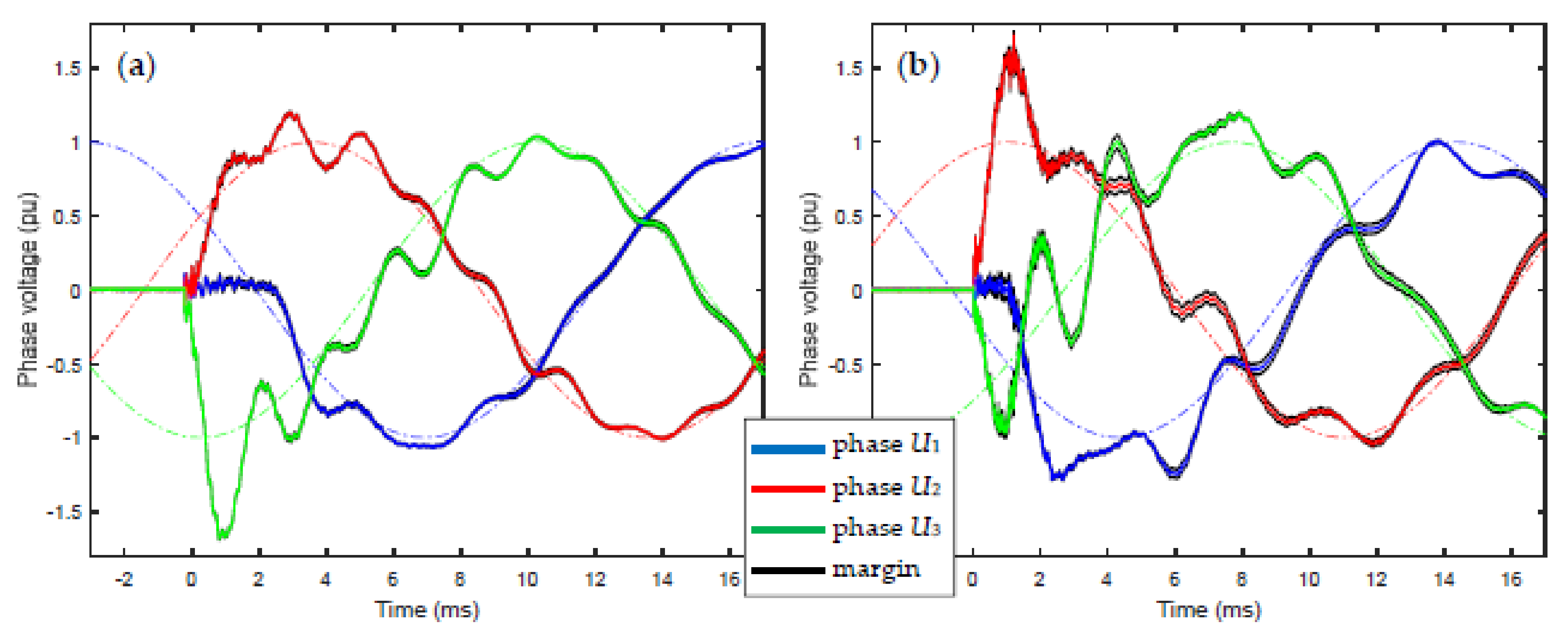
Figure 5 shows the results obtained at the transition points. In both cases the overhead line leaving from the measurement location was energized at its far end. The confidence bounds are significantly smaller compared to those obtained in the substation measurements. Apparently, shielding by the terminations at either side of the sensors reduce cross-coupling significantly. Uncertainties in the cross-coupling therefore have minor effect on the reconstructed waveforms. Also here it was confirmed that the maximum voltages remain within safe limits.

3.2. Reliability of the Reconstructed Waveforms

The D/I measurement results are compared with power system simulations obtained using PSCAD. The studied connection basically consists of a double circuit with 10.8 km cable in between two overhead line sections (4.4 km and 6.8 km length). However, both the magnitude and the harmonic content of switching transient responses depend on a much more extensive part of the grid [9]. The complete Dutch EHV grid was modelled in PSCAD using frequency dependent transmission line models [7,15]. A second measurement campaign was arranged aiming for simultaneously recording using the D/I measurement system and the RC dividers present at the transition points. The comparison allows to judge the sensitivity of different techniques in terms of EMC.

3.2.1. Comparison with PSCAD Simulation

Measurements were conducted at both line to cable transition points and at one of the substations. At each location six switching actions were performed differing in the side from which the connection was energized, the operation state of the parallel circuit and the choice of the parallel circuits to be energized. A selection is presented in Figure 6, corresponding to the results in Figure 4 and Figure 5, with the parallel circuit de-energized.

Figure 6a,b show the result obtained at the substation, where the circuit is excited from the far side and from the measurement side, respectively. Figure 6c,d provide the associated results for the transition points. The excitation of the connection is performed at the overhead line ending at the transition point where measurements are conducted. It can be concluded that measurement results confirm the simulations in large detail.

3.2.2. Comparison with RC Divider Measurement

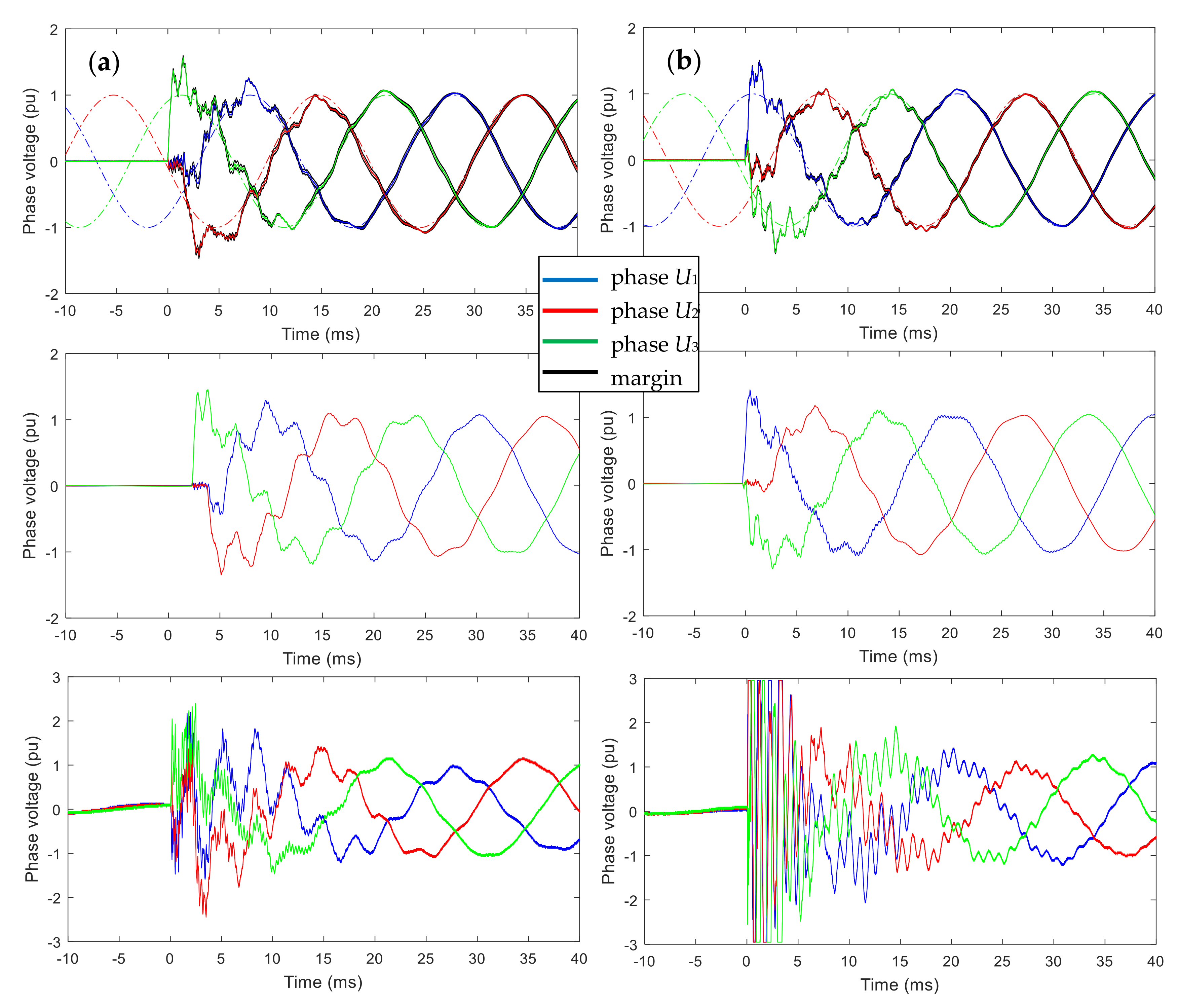
Figure 7 shows the result from simultaneous measurement with the D/I method (top figures) and an RC divider (bottom figures). In between, the PSCAD simulations are presented. The measurements are taken at both transition points with the parallel circuit in service. It is observed that oscillations occur in the divider response, which are far more severe than found in both the simulation and the D/I response. It should be noted that, although simulation and D/I response are quite similar, also here the measured oscillation immediately after energizing is somewhat stronger than simulated.

4. Discussion

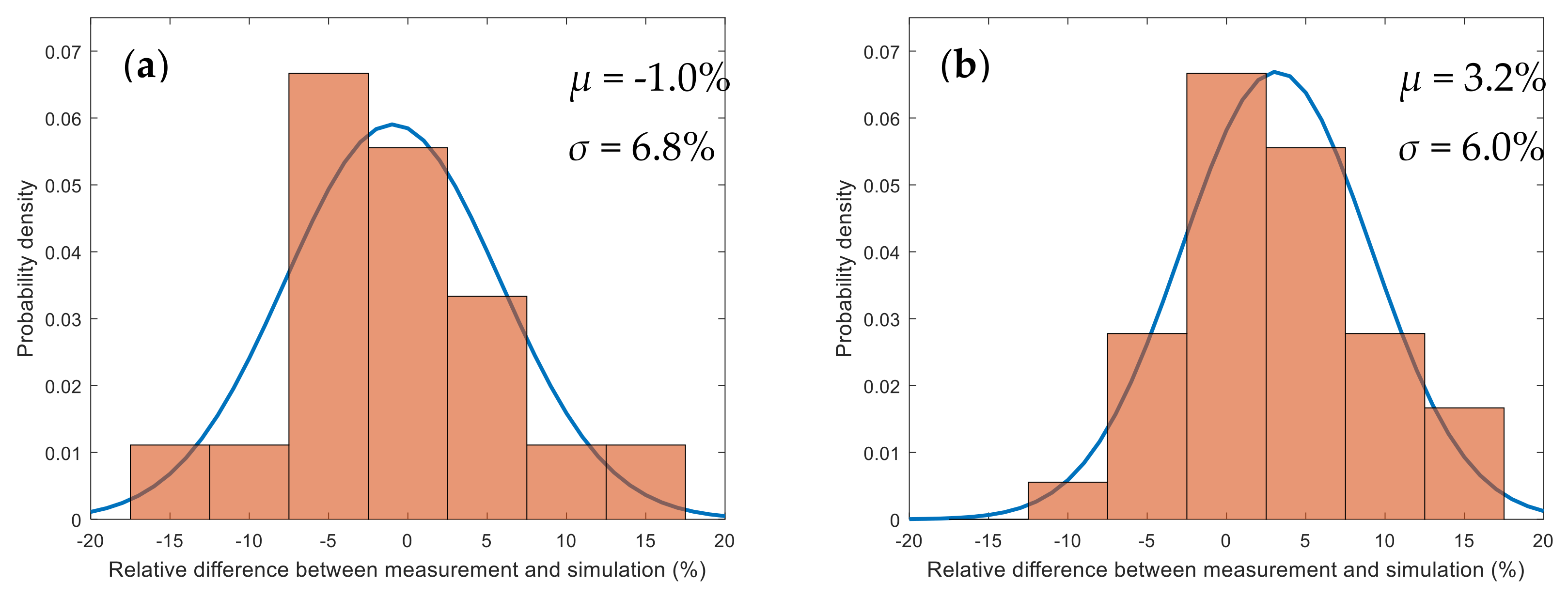
The confidence margins depend on the strength of the cross-couplings and on the accuracy by which they can be determined. For the transition points the contribution of the model uncertainties is about 2%, whereas for the substation it reaches 8% [10]. These uncertainties should be considered when comparing measured and simulated overvoltage magnitudes. Figure 8 shows the statistical distribution of relative differences between simulated and observed maximum overvoltages. The data include six switching actions at all measurement locations, each providing three overvoltage values for the three phases. The width of the fitted normal distributions found for the substation measurement (6.8%, Figure 8a) is only slightly larger as compared to the width for the two transition points (6.0%, Figure 8b). On one hand, this shows that the modelling method is adequate and predicts observations well. On the other hand, it does not represent the difference in measurement accuracy expected from both locations. Apparently, the simulations also contribute to deviations. This is not surprising as, although the complete Dutch EHV grid was simulated in large detail, a number of simplifications were made. Connections to downstream networks (110, 150, 220 kV) were replaced by equivalent impedances based on active and reactive power consumption by the loads according to powerflow calculations [7]. Moreover, connections abroad were not modelled in detail.

The comparison with divider measurements revealed serious differences and apparently EMC is an issue. High frequency components are overrepresented in the divider waveforms, which points to interference related to the signal time derivative. Common mode currents along measurement cables, as discussed in Section 2, can be induced by the time varying magnetic flux caused by ground currents. Poor measurement cable quality and cable layout are suspected to translate the common mode currents into disturbance adding to the recorded waveforms. Also, slight disturbance seems to be picked up by the D/I system. For the measurements presented in Section 3.2 the ground plates of each sensor were connected to the metal support of the termination near the sensor. This causes ground loops formed by the earth screens of the measurement cables, which can pick up magnetic flux from a switching event. For the measurements presented in Section 3.1 all sensor ground plates were connected to a central point, avoiding the occurrence of such loops to a large extent. It shows, that even with the D/I methodology, with its intrinsic good EMC characteristics, every connection detail is important in order to perform disturbance free measurements.

5. Conclusions

The D/I methodology with open-air capacitive sensor is capable of recording switching transients in an EMC harsh environment. However, the decoupling inherent to open-air sensors is a tedious process and may limit its application to specific situations:

• Verification of installed measurement systems in case of doubt or when fast transient overvoltages are expected to occur outside the (R) C divider bandwidth. The D/I method can be designed to have a bandwidth in excess of 5 MHz [2,7].
• Commissioning of a new connection to avoid the need of permanent installation of a costly divider. After an operation time, e.g., to confirm that overvoltages remain within safe limits, there might be no further need for having such dedicated equipment installed.
• Upon a system fault the D/I method can be installed in a short time to verify whether voltage transients occur in the connection and may be involved.

The need of pre-assumptions is an obvious drawback when dealing with significant cross-coupling, which may especially occur at large substations. Future research is directed to reduce the number of assumptions to be made in establishing the coupling matrix. Complete information can be extracted by employing the responses from different sensors upon the front of a switching event (as in [4]) in combination with information provided by the power frequency responses as presented here. Having the topologies of Figure 3 in mind, upon an initial travelling wave on one of the lines, only the response ratios of neighbouring sensors are needed. There are four combinations which, together with information from power frequency fitting, would completely determine the coupling matrix.

References

- Irwin, T.; Ryan, H.M. Insulation co-ordination for AC transmission and distribution systems. In High-Voltage Engineering and Testing, 3rd ed.; Ryan, H.M., Ed.; IET Power and Energy Series; IET: Stevenage, UK, 2013; Volume 66, pp. 61–63. [Google Scholar]
- Barakou, F.; Wouters, P.A.A.F.; Mousavi Gargari, S.; Smit, J.; Steennis, E.F. Merits and challenges of a differentiating-integrating measurement methodology with air capacitors for high-frequency transients. In Proceedings of the CIGRE 2018, Paris, France, 26–31 August 2018. C4-203. [Google Scholar]
- Van Heesch, E.J.M.; van Deursen, A.P.J.; van Houten, M.A.; Jacobs, G.A.P.; Kersten, W.F.J.; van der Laan, P.C.T. Field tests and response of the D/I H.V. measuring system. In Proceedings of the 6th International Symposium on High-Voltage Engineering, New Orleans, LA, USA, 28 August–1 September 1989. [Google Scholar]
- Van Heesch, E.J.M.; Caspers, R.; Gulickx, P.F.M.; Jacobs, G.A.P.; Kersten, W.F.J.; van der Laan, P.C.T. Three phase voltage measurements with simple open air sensors. In Proceedings of the 7th International Symposium on High-Voltage Engineering, Dresden, Germany, 26–30 August 1991. [Google Scholar]
- Smeets, R.P.P.; van der Linden, W.A.; Achterkamp, M.; Damstra, G.C.; de Meulemeester, E.M. Disconnector switching in GIS: Three-phase testing and phenomena. IEEE Trans. Power Deliv. 2000, 15, 122–127. [Google Scholar] [CrossRef]
- Chen, K.-L.; Guo, Y.; Ma, X. Contactless voltage sensor for overhead transmission lines. IET Gener. Transm. Distrib. 2018, 12, 957–966. [Google Scholar] [CrossRef]
- Barakou, F.; Wouters, P.A.A.F.; Mousavi Gargari, S.; de Jong, J.P.W.; Steennis, E.F. Online transient measurements of EHV cable system and model validation. IEEE Trans. Power Deliv. 2019, 34, 532–541. [Google Scholar] [CrossRef]
- EMTDC User’s Guide, 5th ed.; Manitoba HVDC Research Centre Inc.: Winnipeg, MB, Canada, 2010.
- Barakou, F.; Haverkamp, A.R.A.; Wu, L.; Wouters, P.A.A.F.; Steennis, E.F. Investigation of necessary modeling detail of a large scale EHV transmission network for slow front transients. Electr. Power Syst. Res. 2017, 147, 192–200. [Google Scholar] [CrossRef]
- Wouters, P.A.A.F.; Barakou, F.; Mousavi Gargari, S.; Smit, J.; Steennis, E.F. Accuracy of switching transients measurement with open-air capacitive sensors near overhead lines. In Proceedings of the IEEE International Conference on High Voltage Engineering and Application, Athens, Greece, 10–13 September 2018. [Google Scholar]
- Van Deursen, A.P.J.; Smulders, H.W.M.; de Graaff, R.A.A. Differentiating/integrating measurement setup applied to railway environment. IEEE Trans. Instrum. Meas. 2006, 55, 316–326. [Google Scholar] [CrossRef]
- Van der Laan, P.C.T.; van Deursen, A.P.J. Reliable protection of electronics against lightning: Some practical applications. IEEE Trans. Electromagnet. Compat. 1998, 40, 513–520. [Google Scholar] [CrossRef]
- Kuperus, J.; Meten in de fysika IIb. Course material in Dutch 1976. Utrecht University, The Netherlands.
- Brandt, S. Data analysis—Statistical and Computational Methods for Scientists and Engineers, 4th ed.; Springer International Publishing: Cham, Switzerland, 2014; pp. 15–40. [Google Scholar]
- Paul, C.R. Analysis of Multiconductor Transmission Lines, 2nd ed.; John Wiley & Sons Inc.: Hoboken, NJ, USA, 2008. [Google Scholar]
Figure 1.
Measurement topologies for D/I and divider methods. Component values for D/I are such that the receiving cable end represents the time derivative of phase voltage UHV and the waveform is restored by integration (the open-air sensor design is shown on the left); For standard dividers this signal directly represents the phase voltage UHV.
Figure 2.
Effect of induced ground currents along the measurement cable (left); Through the cable transfer impedance the resulting common mode current ICM causes a differential mode voltage UDM which divides over the impedances at the cable ends (right).
Figure 3.
Topologies and sensor (ui) positioning with respect to phase voltages Uj: (a) Overhead line ending at a substation, photo shows the installation of the sensors; (b) Overhead line to underground power cable transition (with termination T, surge arrester S.arr. and voltage transformer V.tr.), photos show the sensor (as seen from below) and its positioning in between two terminations belonging to the same phase. The sensor heights (indicated with arrows) are always chosen such, that they remain below the height reached by the supporting structures of the terminations.
Figure 4.
Reconstructed waveforms for substation measurements recorded with 5 Msample/s over a duration corresponding to ten power cycles. The curves in colour represent the three phases with confidence margins in black: (a) Full and 10 times zoomed waveform showing overvoltages during the first cycle from energization at the far end of the connection; (b) Waveform with overvoltages during the first power cycle from energization at the near end and 10 times zoomed waveform revealing initial travelling waves along the connection. The extrapolated power cycles (dash-dotted lines) indicate the 50 Hz phase angles at the moments of contact.
Figure 5.
Part of the reconstructed waveforms (covering 10 cycles recorded with 5 Msample/s) around the switching moment for measurement at transition points. Coloured curves represent the phase voltages with one standard deviation confidence margins indicated in black: (a) Overvoltages from energization at the substation connected by 4.4 km overhead line to the transition point; (b) Overvoltages from energization at the substation connected via 6.8 km overhead line. Moments of contact can be observed from the extrapolated power frequency waveforms (dash-dotted lines).
Figure 6.
Comparison between D/I measurement (continuous lines in colour for the three phases) and PSCAD simulations (dash-dotted black lines). Generally, the maximum overvoltage value observed for each switching event and phase agree well with calculations for: (a) Recording at substation with energization from far end substation; (b) Recording and energization at the same substation; (c) Energization at substation 4.4 km from the observed transition point; (d) Energization from substation at 6.8 km from the observed transition point.
Figure 7.
Comparison of results from D/I methodology (top figures, black lines indicate the uncertainty margins caused by uncertainty in decoupling), PSCAD simulation (middle figures) and RC-divider results (bottom figures): (a) Energization from substation connected by 4.4 km overhead line to the transition point; (b) Energization from substation connected via 6.8 km overhead line. For both switching events the high frequency oscillations are overrepresented in the divider measurement as compared to both D/I measurement and simulation.
Figure 8.
Comparison of measurement and simulation for transition overvoltages upon energizing from nearby substation: (a) Results for the substation; (b) Results for the two transition points.
© 2019 by the authors. Licensee MDPI, Basel, Switzerland. This article is an open access article distributed under the terms and conditions of the Creative Commons Attribution (CC BY) license (http://creativecommons.org/licenses/by/4.0/).
Share and Cite
MDPI and ACS Style
Barakou, F.; Steennis, F.; Wouters, P. Accuracy and Reliability of Switching Transients Measurement with Open-Air Capacitive Sensors. Energies 2019, 12, 1405. https://doi.org/10.3390/en12071405
AMA Style
Barakou F, Steennis F, Wouters P. Accuracy and Reliability of Switching Transients Measurement with Open-Air Capacitive Sensors. Energies. 2019; 12(7):1405. https://doi.org/10.3390/en12071405
Chicago/Turabian StyleBarakou, Fani, Fred Steennis, and Peter Wouters. 2019. "Accuracy and Reliability of Switching Transients Measurement with Open-Air Capacitive Sensors" Energies 12, no. 7: 1405. https://doi.org/10.3390/en12071405
Note that from the first issue of 2016, this journal uses article numbers instead of page numbers. See further details here.