Multi-Dimensional Performance Evaluation of Heat Exchanger Surface Enhancements

Abstract

Enhanced heat transfer surfaces allow more energy-efficient, compact and lightweight heat exchangers. Within this study, a method for comparing different types of enhancement and different geometries with multiple objectives is developed in order to evaluate new and existing enhancement designs. The method’s objectives are defined as energy, volume, and mass efficiency of the enhancement. They are given in dimensional and non-dimensional form and include limitations due to thermal conductivity within the enhancement. The transformation to an explicit heat transfer rate per dissipated power, volume, or mass is described in detail. The objectives are visualized for different Reynolds numbers to locate beneficial operating conditions. The multi-objective problem is further on reduced to a single-objective problem by means of weighting factors. The implementation of these factors allows a straightforward performance evaluation based on a rough estimation of the energy, volume, and mass importance set by a decision maker.

1. Introduction

Heat transfer enhancements improve heat exchanger efficiencies in many industrial, domestic, and transport applications. In particular, savings in energy demand, volume, and material mass drive the development of new enhancement structures. Applications with high fan power consumption, such as air-cooled condensers in power plants or outdoor units of air source heat pumps, profit from reduced fluid friction and pressure drop. Applications with limited space and mobile operation, such as cars or airplanes, profit from compact and lightweight heat transfer enhancements, respectively. Various enhanced surfaces arose from these and numerous other applications. Stone [1] denominates their main purposes as

• increasing the compactness of heat exchangers in order to reduce their overall volume, material, and possibly their cost,
• reducing the pumping/fan power required for a given heat transfer process, and/or
• increasing the overall UA value of the heat exchanger.

Those purposes are linked straightforward to the objectives of a specific maximum heat transfer rate at a specific minimum power consumption, volume and mass [2]. The optimal decision on the choice of an enhancement needs to be made in the presence of trade-offs between these conflicting objectives. The optimal heat exchanger enhancement design with a focus on volume would consist of very dense structures with a high surface area in the available volume; however, fluid friction could be very large. Focusing on mass-reduced enhancements would result in very fine structures with high heat transfer coefficients on the surface, with the possible drawback of limitations in heat conduction through the enhancement and high fluid friction.

Several different methods are described in the literature on the evaluation of heat exchanger performance. As the benefits and drawbacks of a surface change can be very complex and multidimensional, a simple method of performance evaluation will not be comprehensive. The focus of this discussion shall be on different evaluation methods in the literature and the integration of (i) a heat transfer limitation due to low thermal conductivity through the fins and (ii) variable objectives within the method. The former information (i) is necessary for a broader study of geometry variation of surface area enhancements; the enhancement yields, at some geometrical design point, always a limitation of the heat transfer due to low thermal conductivity of the fins. If this is not represented in an evaluation method, the feasible set of possible geometries must be specified very restrictively.

Stone [1] gives a comprehensive review of existing methods, simple as well as more complex ones. The method of “j and f vs. curves” is among them. It shows curves of the Colburn factor j and the friction factor f, plotted versus the Reynolds number or the reciprocal of an equivalent diameter. The values tend to vary over a wide range [3] or have a large scattering, such that the method is applicable with restrictions [1]. The fin efficiency or an equivalent description of conductivity through the fins is not part of the method.

A second method describes the goodness criteria [4]. In the area goodness factor method, the ratio of the Colburn factor and the Fanning friction factor is plotted versus the Reynolds number. The consequence of this definition is that “a surface having a higher $j/f$ factor is good because it will require a lower free-flow area and hence a lower frontal area for the exchanger” ([5], p. 705). However, “no significant variation is found in the $j/f$ ratio” ([5], p. 705), such that the free-flow area is hardly changing for various surfaces. However, the volume of a heat exchanger is very sensitive to a surface change. The volume goodness factor for surfaces with different characteristic lengths expresses the capability to transfer heat (${\eta }_0{h}_{\mathrm{std}}\beta$) versus the dissipated power per volume ($E_{\mathrm{std}}\beta$). The same fluid flow rate is required for comparison. Then, “for constant $E_{\mathrm{std}}\beta$, a surface having a high plot of ${\eta }_0{h}_{\mathrm{std}}\beta$ vs. $E_{\mathrm{std}}\beta$ is characterized as the best from the viewpoint of heat exchanger volume” ([5], p. 707). A screening method is presented by Webb and Kim [6] with a collection of performance evaluation criteria (PEC). They are partitioned into fixed geometry (FG), fixed flow area (FN), and variable geometry (VG) criteria. The idea is to replace a plain surface by an enhanced surface, while keeping some boundary conditions constant and, thereafter, to compare the thermal-hydraulic characteristics. In the general description of the method, the conductivity through the fins is included, as e.g., the heat transfer rate is used as an objective to be maximized ([5], p. 714). However, in a later expression of performance evaluation criteria ([5], p. 715ff) with enhanced surfaces compared to a plain surface, the conductivity through the fins is neglected.

Two dimensionless performance parameters are defined by LaHaye et al. [3] referring to the j and f vs. curves method. The two parameters are the heat transfer performance factor $J=j\mathrm{Re}$ and the pumping power factor $F=f{\mathrm{Re}}^3$. The parameters are plotted versus each other. The effects of fin thickness (and thermal conductivity through the fin) have not been accounted for in that method.

The extension of this method by Soland [7] with reference to more general dimensions of the heat exchanger (plate-fin) also lacks in inclusion of the fin efficiency. The benefit of the method is that a “comparison of many surfaces to a single common smooth plate nominal diameter permits a relative comparison between surfaces having different nominal diameters” ([7], p. 38). Several different types of plate-fin surfaces can be considered with this method.

The general comparison methods developed by Cowell [8] show “how measures for the relative value of required hydraulic diameter, frontal area, total volume, pumping power, and number of transfer units for different surfaces can be derived and displayed” [8]. Two or three of these parameters are kept constant, while the others can be varied and calculated based on the formulas given by Cowell. The effects of the fin efficiency are ignored.

Sahiti et al. [9] suggest to show the quotient of the heat transfer rate and the heat exchanger volume versus the quotient of the required power input and the heat exchanger volume. This method resembles the ranking performance method [7] and uses the number of transfer units to continue calculation of the heat transfer rate. Wherever possible, Sahiti et al. recommend to take into account the additional thermal resistances (fins, second fluid) in the calculation of the number of transfer units.

A comparison of enhancements with some of the methods above is given in [10] for a variety of enhancements. Marthinuss [11] compares five different enhancements given in [5], including volume and mass efficiency.

Table 1 shows a summary of the main assets and the integration of thermal conductivity through the fins of the methods presented above.

Table 1. Methods for performance evaluation retrieved from the literature, with the main assets and information on whether thermal conductivity of the fins is integrated in the method or not.

Method	Sources	Assets	Inclusion of Conductivity of Fins
j and f vs. curves	[1,3]	simple visualization of the thermal-hydraulic performance	no
Area goodness factor	[1,5]	identification of feasible surfaces with low free-flow area	no
Volume goodness factor	[5]	identification of feasible surfaces with low volume	yes
Performance evaluation criteria (PEC)	[5,6]	designer-specific choice of evaluation criteria	(yes) *
Performance parameters	[1,3]	convenient method for comparing various heat transfer geometries in one figure	no
Ranking performance	[7]	comparison of very different fin types with respect to different designer conditions	no
General comparison method	[8]	designer-specific choice of evaluation criteria	no
Energetic comparison	[9]	no volume or surface geometry constraints	yes

* The general formulation includes thermal conductivity of the fins.

From the literature review, a lack in performance evaluation methods including thermal conductivity within the fins can be seen. However, the two methods of volume goodness factor [5] and energetic comparison [9] consider the thermal conductivity. However, they have drawbacks in the choice of the objectives, the fundamental concepts of the methods shall be taken and extended in the following analysis. The extension includes an evaluation of the dissipated power, volume, and mass with respect to the heat transferred.

In the first part of this study, we present a method to evaluate the thermal performance in relation to energy, volume, and mass. The novelty of this approach is a very clear relation of the defined non-dimensional performance figures with the dimensional objectives of a decision maker. The method is suitable for correlation data, measurement data, and simulation data. The definition of key figures renounces the use of a characteristic length and, thus, the performance evaluation method allows a clearer comparison of different enhancements. In the Results part, the method is exemplarily applied to three different enhancements. The multi-objective problem is thereafter reduced to a single-objective problem. The importance of energy, volume, and mass savings can be stated by giving a weighting to each of the three savings.

In summary, the reader will have a tool:

• to optimize a surface enhancement geometry (topology),
• to compare different surface enhancements with each other, and
• to control the main restrictions on energy, volume, and mass use for the optimization/comparison.

2. Performance Evaluation Criteria for Surface Area Enlargement

2.1. Multi-Dimensional Performance Evaluation Criteria

Multi-dimensional performance evaluation criteria would allow a many-faceted view on heat exchanger surface enhancements. However, a too broad view on a subject prevents a clear understanding of coherences. Thus, a multi-dimensional approach requires restrictions. In this study, the focus is on one fluid side (fluid 1) and several restrictions are set on the heat exchanger surface enhancement comparison. When two or more surface enhancements shall be compared, the comparison should take place at a specified thermal-hydraulic scale. That means the performance is evaluated for

• the same heat transfer fluids,
• the same mean fluid temperatures T and pressures p,
• the same mass flow rates $\dot{m}$,
• the same heat transfer rates $\dot{Q}$,
• the same small thermal resistances on the second fluid side.

The values above can be chosen arbitrarily, but must then be fixed. The compared heat exchangers might differ in the actual design costs, defined as

• dissipated power $P_{\mathrm{diss}}$,
• structure volume $V_{\mathrm{st}}$,
• structure mass $m_{\mathrm{st}}$.

The restrictions (1) to (5) above hold for the performance comparison. This does not mean that the heat exchanger surface enhancements must be experimentally tested at this specified thermal-hydraulic scale. On the contrary, the non-dimensional performance evaluation criteria which will be defined, will allow a broad evaluation based on limited information.

The development of the method will be based on air as fluid 1, but can be transferred to other fluids. The dissipated power $P_{\mathrm{diss}}=\Delta p_{\mathrm{st}}{\dot{V}}_{\mathrm{air},\mathrm{st}}$ is the product of the pressure drop within the core structure $\Delta p_{\mathrm{st}}$ (cf. Equation (A1)) and the volume flow rate through the structure ${\dot{V}}_{\mathrm{air},\mathrm{st}}$. The relation to the electric power consumption $P_{\mathrm{el}}$ is given by $P_{\mathrm{diss}}={\eta }_{\mathrm{fan},\mathrm{system}}{P}_{\mathrm{el}}$. The fan system efficiency ${\eta }_{\mathrm{fan},\mathrm{system}}$ includes the aerodynamic, mechanical, and motor losses. The structure volume $V_{\mathrm{st}}$ is equal to the product of the structure frontal area $A_{\mathrm{in},\mathrm{st}}$ and the structure length $L_{\mathrm{st}}$. In this study, the focus is on the comparison of heat exchangers with equal $A_{\mathrm{in},\mathrm{st}}$ (and thus equal velocities through the structure), but is not limited to this. Both parameters $A_{\mathrm{in},\mathrm{st}}$ and $L_{\mathrm{st}}$ can vary.

With the above restrictions, the mean fluid properties for the compared heat exchangers are equal and the heat transfer rate $\dot{Q}$ can be expressed by

$$\begin{array}{c}\hfill \dot{Q}={\eta }_{0}h{A}_{\mathrm{HTS}}\Delta T_{\mathrm{m}},\end{array}$$

(1)

with the extended surface efficiency ${\eta }_0$ (cf. [5], p. 289), the heat transfer coefficient h, the heat transfer surface area $A_{\mathrm{HTS}}$, and the mean temperature difference between the fluids $\Delta T_{\mathrm{m}}$.

Simplification allows comparing the heat exchangers at equal ${\eta }_{0}h{A}_{\mathrm{HTS}}$, instead of equal heat transfer rate $\dot{Q}$, as long as $\Delta T_{\mathrm{m}}$ in Equation (1) is constant (which is ensured by restrictions (1) to (5)). The product ${\eta }_{0}h{A}_{\mathrm{HTS}}$ is defined as benefit of the heat transfer process and it is related to different costs in (i) a dimensional straightforward way and in (ii) a non-dimensional way allowing more general statements.

2.1.1. Definition of Dimensional Evaluation Criteria

The dimensional criteria shall relate the benefit to different types of costs, which are linked to operational costs (e.g., driven by the dissipated power or mass), investment costs (e.g., driven by the volume or mass), and the driving temperature difference $\Delta T_{\mathrm{m}}$. Details are given in Table 2. This is a straightforward non-novel way for the energy efficiency ${ϵ}_{\mathrm{E}}$, related to e.g., the volume goodness factor [5] and the energetic comparison [9]. Repeating this ansatz for the volume and mass efficiency is helpful to allow performance quantities with the same pattern for better understandability. Similar quantities are defined in [11].

Table 2. Key figures for extended performance evaluation; defined as benefit ${\eta }_0{h}_{\mathrm{air}}{A}_{\mathrm{HTS}}$ per cost. The main definition and the alternative definition are equal, but differ in the input parameters.

Cost	Key Figure	Main Definition	Alternative Definition	Dimension
Dissipated power on the air-side $\Delta p_{\mathrm{st}}{\dot{V}}_{\mathrm{air},\mathrm{st}}$ in $\mathrm{W}$, which is proportional to the electric power consumption of the fans	Energy efficiency ${ϵ}_{\mathrm{E}}$	$\frac{{\eta }_0{h}_{\mathrm{air}}{A}_{\mathrm{HTS}}}{\Delta p_{\mathrm{st}}{\dot{V}}_{\mathrm{air},\mathrm{st}}}$	$\frac{\dot{Q}}{P_{\mathrm{diss}}}\frac{1}{\Delta T_{\mathrm{m}}}$	1/$\mathrm{K}$
Available volume for heat transfer enhancement $V_{\mathrm{st}}$ in ${\mathrm{m}}^3$ (excluding fluid guidance volume and header/distributor)	Volume efficiency ${ϵ}_{\mathrm{V}}$	$\frac{{\eta }_0{h}_{\mathrm{air}}{A}_{\mathrm{HTS}}}{V_{\mathrm{st}}}$	$\frac{\dot{Q}}{V_{\mathrm{st}}}\frac{1}{\Delta T_{\mathrm{m}}}$	$\mathrm{W}/\left({\mathrm{m}}^3\mathrm{K}\right)$
Material usage for the wire or fin structure $m_{\mathrm{st}}$ in kg (excluding fluid guidance, solder material and header/distributor)	Mass efficiency ${ϵ}_{\mathrm{M}}$	$\frac{{\eta }_0{h}_{\mathrm{air}}{A}_{\mathrm{HTS}}}{m_{\mathrm{st}}}$	$\frac{\dot{Q}}{m_{\mathrm{st}}}\frac{1}{\Delta T_{\mathrm{m}}}$	$\mathrm{W}$/($\mathrm{k}$$\mathrm{g}$$\mathrm{K}$)

These key figures can be presented based on performance measurement data or correlations found in the literature. However, a comparison with the restrictions (1) to (5) requires equal temperature and pressure conditions, which are difficult to achieve during measurement. Thus, a non-dimensioning of the defined key figures could allow a more easy implementation of data, with the drawback of a less accessible output.

2.1.2. Definition of Non-Dimensional Evaluation Criteria

The transformation from dimensional into non-dimensional evaluation criteria requires parameters such as the Reynolds number

$${\mathrm{Re}}_{\mathrm{st}}=\frac{v_{\mathrm{st}}{d}_{\mathrm{st}}}{{\nu }_{\mathrm{air},\mathrm{st}}},$$

(2)

the Nusselt number

$${\mathrm{Nu}}_{\mathrm{air}}=\frac{h_{\mathrm{air}}{d}_{\mathrm{st}}}{k_{\mathrm{air},\mathrm{st}}},$$

(3)

the Fanning friction factor (cf. Appendix A)

$${\mathrm{f}}_{\mathrm{st}}=\frac{d_{\mathrm{st}}}{4L_{\mathrm{st}}}\left[\frac{2\Delta p_{\mathrm{HX}}}{{\rho }_{\mathrm{air},\mathrm{st}}{v}_{\mathrm{st}}^2}-\left(K_{\mathrm{c}}+K_{\mathrm{e}}\right)\right],$$

(4)

the surface area density

$$\beta =\frac{A_{\mathrm{HTS}}}{V_{\mathrm{st}}},$$

(5)

and the structure porosity

$${\phi }_{\mathrm{st}}=\frac{V_{\mathrm{st}}-V_{\mathrm{st},\mathrm{mat}}}{V_{\mathrm{st}}}.$$

(6)

The dependencies of the non-dimensional parameters ${\mathrm{Nu}}_{\mathrm{air}}$, $f_{\mathrm{st}}$, and ${\eta }_0$ on each other and on additional parameters are given in Appendix D.

The non-dimensional energy efficiency ${ϵ}_{\mathrm{E}}^{*}$ will now be defined. It is a novel combination of area and volume goodness factor [5] and the dimensional energy efficiency ${ϵ}_{\mathrm{E}}$. The basic principle is based on a separation of $\dot{Q}/P_{\mathrm{diss}}$ into a product of two parameters; the driving parameter $F_{\mathrm{Driving}}$ for the process and the non-dimensional energy efficiency ${ϵ}_{\mathrm{E}}^{*}$:

$$\frac{\dot{Q}}{P_{\mathrm{diss}}}=F_{\mathrm{Driving}}{ϵ}_{\mathrm{E}}^{*}.$$

(7)

The driving parameter has to be chosen in such a way, that a fair comparison of different heat exchangers takes place when considering ${ϵ}_{\mathrm{E}}^{*}$.

For the dimensional evaluation criteria in Table 2, the driving parameter has been defined as $\Delta T_{\mathrm{m}}$. Thus, a specific heat exchanger, measured at two different $\Delta T_{\mathrm{m}}$ shows the same value for the energy efficiency ${ϵ}_{\mathrm{E}}$, even though $\dot{Q}/P_{\mathrm{diss}}$ might not be the same. Restrictions (1), (2), (3), and (5) must be ensured during measurement to allow this. Thus, ${ϵ}_{\mathrm{E}}$ is trivially a better performance quantity than $\dot{Q}/P_{\mathrm{diss}}$; however, the data generation to calculate ${ϵ}_{\mathrm{E}}$ is restricted.

A performance evaluation with a less restricted data generation takes into account the change of e.g., type of heat transfer fluid, the change of material properties due to a temperature or pressure variation, and the change of the mass flow rate due to a variation in heat exchanger size. Based on the Buckingham $\pi$ theorem, there are now several options to express the driving parameter $F_{\mathrm{Driving}}$ and the non-dimensional energy efficiency ${ϵ}_{\mathrm{E}}^{*}$, such that ${ϵ}_{\mathrm{E}}^{*}$ is a function of non-dimensional quantities only (Nusselt number, friction factor,…) and fulfill the requirements above. We have chosen the following definition:

$$\begin{array}{cc}\hfill {ϵ}_{\mathrm{E}}^{*}& =\frac{{\mathrm{Nu}}_{\mathrm{air}}}{2{\mathrm{f}}_{\mathrm{st}}}{\eta }_0\frac{d_{\mathrm{st}}\beta }{{\mathrm{Re}}_{\mathrm{st}}},\hfill \end{array}$$

(8)

$$\begin{array}{cc}\hfill F_{\mathrm{Driving}}& =\frac{k_{\mathrm{air},\mathrm{st}}\Delta T_{\mathrm{m}}}{{\mu }_{\mathrm{air},\mathrm{st}}{v}_{\mathrm{st}}^2}=\frac{1}{\mathrm{Br}},\hfill \end{array}$$

(9)

with Brinkman number

$$\mathrm{Br}=\frac{{\mu }_{\mathrm{air},\mathrm{st}}{v}_{\mathrm{st}}^2}{k_{\mathrm{air},\mathrm{st}}\Delta T_{\mathrm{m}}}.$$

(10)

Thereof, it follows directly:

$${ϵ}_{\mathrm{E}}^{*}=\frac{\dot{Q}}{P_{\mathrm{diss}}}\mathrm{Br}.$$

(11)

The Brinkman number expresses the ratio between the viscous dissipation power and the heat transported by molecular conduction. Based on restrictions (1) to (5), the Brinkman number is equal for the comparison of different heat exchangers with equal structure frontal area $A_{\mathrm{in},\mathrm{st}}$. From the right-hand side term in Equation (11), the idea of ${ϵ}_{\mathrm{E}}^{*}$ should become clearer: The benefit versus cost ratio of $\dot{Q}$ and $P_{\mathrm{diss}}$ is reduced by each driving force, which is $k_{\mathrm{air},\mathrm{st}}\Delta T_{\mathrm{m}}$ on the thermal side and ${\mu }_{\mathrm{air},\mathrm{st}}{v}_{\mathrm{st}}^2$ on the dynamic side. The higher the parameter ${ϵ}_{\mathrm{E}}^{*}$, the less power is dissipated.

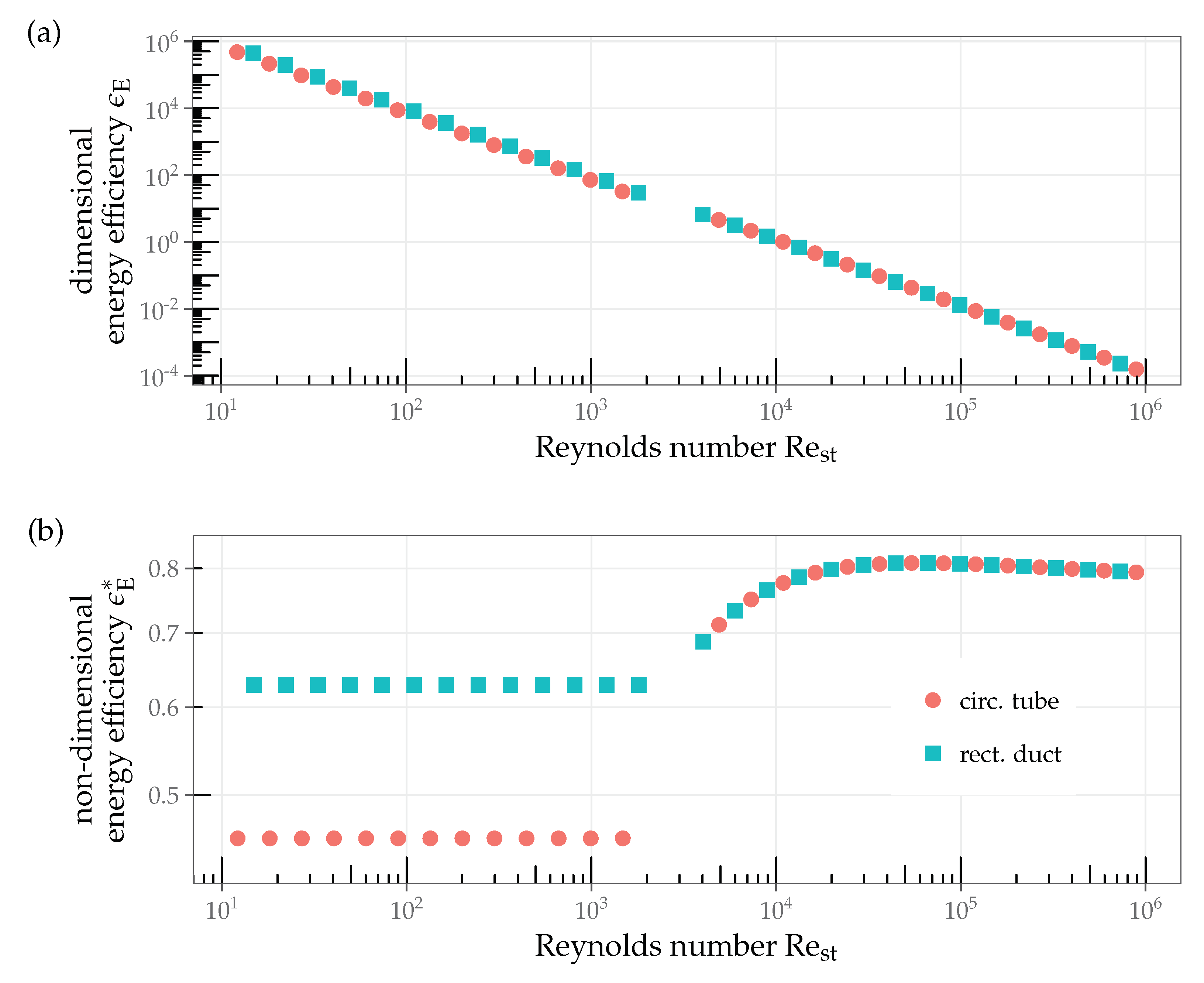
The value of ${ϵ}_{\mathrm{E}}^{*}$ has no evident upper limit. For a fully developed laminar flow through a smooth circular tube, ${ϵ}_{\mathrm{E}}^{*}$ equals 0.46. For a fully developed laminar flow through a rectangular duct of zero aspect ratio, ${ϵ}_{\mathrm{E}}^{*}$ equals 0.63. For the turbulent flow, ${ϵ}_{\mathrm{E}}^{*}$ is bounded by 0.81 for both geometries. The thermal-hydraulic correlations used to calculate these values are given in ([5], p. 476, p. 482): ${\mathrm{Nu}}_T=3.7$, ${\mathrm{Nu}}_T=7.5$ and $f\mathrm{Re}=16$, $f\mathrm{Re}=24$ for the laminar case of the circular tube and rectangular duct, respectively; and the Bhatti–Shah and Gnielinski correlations for the turbulent case for both geometries. The curves are shown in Figure 1b for a Reynolds number based on a hydraulic diameter in the range of $10\le {\mathrm{Re}}_{\mathrm{st}}\le {10}^6$. The value of ${ϵ}_{\mathrm{E}}^{*}$ for the laminar case is constant; the value for the turbulent case increases first, with a maximum at ${\mathrm{Re}}_{\mathrm{st}}=6\times {10}^4$, and slowly decreases thereafter. The transition regime in the range of $2000\le {\mathrm{Re}}_{\mathrm{st}}\le 4000$ is not shown due to strong differences within different correlations in this regime. A comparison between heat exchangers takes place at constant (or similar) Reynolds numbers (cf. restrictions (1) to (5)). Thus, Figure 1b should not misdirect to a statement on whether turbulent flow is more energy efficient than laminar flow. In order to emphasize this point, Figure 1a shows the dimensional energy efficiency defined in Table 2. However, Figure 1b shows for a bandwidth of Reynolds numbers that a rectangular duct shall be preferred as a heat exchanger geometry, when considering energetic performance. Furthermore, Figure 1b has the important benefit of presenting a performance comparison for different Reynolds numbers and keeping the performance quantity ${ϵ}_{\mathrm{E}}^{*}$ in the same scale.

Figure 1. Dimensional (a) and non-dimensional (b) energy efficiency ${ϵ}_{\mathrm{E}}$ and ${ϵ}_{\mathrm{E}}^{*}$, respectively, versus Reynolds number ${\mathrm{Re}}_{\mathrm{st}}$ for a fully developed laminar and turbulent flow in a smooth circular tube and a rectangular duct; air is used in (a) as fluid at 25 ${}^{\circ }\mathrm{C}$ and 1 atm with a hydraulic diameter of 5 $\mathrm{m}$$\mathrm{m}$; the transition flow is not shown. Data is based on [5].

The non-dimensional way of accounting for energetic performance is given in Table 3 with additional calculation formulas for ${ϵ}_{\mathrm{E}}^{*}$. The volume and mass efficiencies are included as well. Their derivation is given in Appendix B. Similarly to the definition of ${ϵ}_{\mathrm{E}}^{*}$, the fraction $\dot{Q}/V_{\mathrm{st}}$ is the product of the non-dimensional volume efficiency ${ϵ}_{\mathrm{V}}^{*}$ and a driving parameter $v_{\mathrm{st}}^2{k}_{\mathrm{air},\mathrm{st}}\Delta T_{\mathrm{m}}/{\nu }_{\mathrm{air},\mathrm{st}}^2$; and $\dot{Q}/m_{\mathrm{st}}$ is the product of the non-dimensional mass efficiency ${ϵ}_{\mathrm{M}}^{*}$ and another driving parameter $v_{\mathrm{st}}^2{k}_{\mathrm{air},\mathrm{st}}\Delta T_{\mathrm{m}}/{\rho }_{\mathrm{air},\mathrm{st}}{\nu }_{\mathrm{air},\mathrm{st}}^2$.

Table 3. Non-dimensional key figures for extended performance evaluation.

Description	Key Figure	Definition	Relation to Dimensional Parameter	Reduced Expression
Energy efficiency	${ϵ}_{\mathrm{E}}^{*}$	$\frac{\dot{Q}}{P_{\mathrm{diss}}}\frac{{\mu }_{\mathrm{air},\mathrm{st}}{v}_{\mathrm{st}}^2}{k_{\mathrm{air},\mathrm{st}}\Delta T_{\mathrm{m}}}$	${ϵ}_{\mathrm{E}}\frac{{\mu }_{\mathrm{air},\mathrm{st}}{v}_{\mathrm{st}}^2}{k_{\mathrm{air},\mathrm{st}}}$	$\frac{{\mathrm{Nu}}_{\mathrm{air}}}{2{\mathrm{f}}_{\mathrm{st}}}{\eta }_0\frac{d_{\mathrm{st}}\beta }{{\mathrm{Re}}_{\mathrm{st}}}$
Volume efficiency	${ϵ}_{\mathrm{V}}^{*}$	$\frac{\dot{Q}}{V_{\mathrm{st}}}\frac{{\nu }_{\mathrm{air},\mathrm{st}}^2}{v_{\mathrm{st}}^2{k}_{\mathrm{air},\mathrm{st}}\Delta T_{\mathrm{m}}}$	${ϵ}_{\mathrm{V}}\frac{{\nu }_{\mathrm{air},\mathrm{st}}^2}{v_{\mathrm{st}}^2{k}_{\mathrm{air},\mathrm{st}}}$	$\frac{{\mathrm{Nu}}_{\mathrm{air}}}{{\mathrm{Re}}_{\mathrm{st}}}{\eta }_0\frac{d_{\mathrm{st}}\beta }{{\mathrm{Re}}_{\mathrm{st}}}$
Mass efficiency	${ϵ}_{\mathrm{M}}^{*}$	$\frac{\dot{Q}}{m_{\mathrm{st}}}\frac{{\rho }_{\mathrm{air},\mathrm{st}}{\nu }_{\mathrm{air},\mathrm{st}}^2}{v_{\mathrm{st}}^2{k}_{\mathrm{air},\mathrm{st}}\Delta T_{\mathrm{m}}}$	${ϵ}_{\mathrm{M}}\frac{{\rho }_{\mathrm{air},\mathrm{st}}{\nu }_{\mathrm{air},\mathrm{st}}^2}{v_{\mathrm{st}}^2{k}_{\mathrm{air},\mathrm{st}}}$	$\frac{{\mathrm{Nu}}_{\mathrm{air}}}{{\mathrm{Re}}_{\mathrm{st}}}{\eta }_0\frac{d_{\mathrm{st}}\beta }{{\mathrm{Re}}_{\mathrm{st}}}\frac{{\rho }_{\mathrm{air},\mathrm{st}}}{{\rho }_{\mathrm{st}}(1-{\phi }_{\mathrm{st}})}$

From the “reduced expression” in Table 3 and Appendix C and Appendix D, it can be seen that all three efficiencies ${ϵ}^{*}$ are solely dependent on the Reynolds number ${\mathrm{Re}}_{\mathrm{st}}$, on the ratio of the thermal conductivities $k_{\mathrm{air},\mathrm{st}}/k_{\mathrm{st}}$, on the Prandtl number, and on the non-dimensional geometry. The key figure ${ϵ}_{\mathrm{M}}^{*}$ is, in addition, dependent on the ratio of the densities ${\rho }_{\mathrm{air},\mathrm{st}}/{\rho }_{\mathrm{st}}$.

Further inspection of ${ϵ}^{*}$ shows that they are defined such that they are independent on the choice of the characteristic length. Thus, for a fixed geometry, fixed values from restrictions (1) to (5), and for any choice of characteristic length $d_{\mathrm{st}}$, the values of ${ϵ}^{*}$ are equal. It is crucial to understand that

• the generation of the non-dimensional efficiencies is independent of the restrictions (1) to (5)
• a comparison of non-dimensional efficiencies of different heat transfer surface enhancements is based on the restrictions (1) to (5)

A thermal-hydraulic performance evaluation of different heat exchangers must take place on the same thermal-hydraulic scale (restrictions (1) to (5)). Thus, at equal $A_{\mathrm{in},\mathrm{st}}$, the comparison is made at equal superficial air velocities $v_{\mathrm{st}}$. However, in the non-dimensional expressions, this does not coincide with equal Reynolds numbers ${\mathrm{Re}}_{\mathrm{st}}$, due to possibly different values for the choice of characteristic length. For later comparisons, a common diameter must be defined for the Reynolds number, such that a comparison is straightforward. As stated by Soland ([7], p. 38), a single common smooth plate nominal diameter could be chosen, representing the distance of the tubes. This recommendation is followed in this study. In general, it is allowed for each comparison to define a new common diameter. In order to distinguish between the diameters, we refer to $d_{\mathrm{mi}}$ as a diameter on the micro-level, usually related to the performance correlations and specific for each heat exchanger structure. $d_{\mathrm{ma}}$ is referred to as a diameter on the macro-level, usually related to the specific task for comparison, with a stronger relation to the overall dimension of the heat exchanger, and equal for all compared heat exchangers. The different diameters $d_{\mathrm{mi}}$ and $d_{\mathrm{ma}}$ can be used as characteristic lengths in the Reynolds number. The index of ${\mathrm{Re}}_{\mathrm{st}}$ will be extended to ${\mathrm{Re}}_{\mathrm{st},\mathrm{mi}}$ and ${\mathrm{Re}}_{\mathrm{st},\mathrm{ma}}$, respectively. Figure 2 shows three different heat exchangers and the method of comparison. The efficiency curves of the heat exchangers show the efficiency ${ϵ}^{*}$ in terms of these modified Reynolds numbers. A comparison of curves at equal ${\mathrm{Re}}_{\mathrm{st},\mathrm{ma}}$ allows the evaluation of performance differences. The higher the values of ${ϵ}^{*}$, the lower is the cost in terms of energy, volume, or mass (at equal heat transfer rate $\dot{Q}$).

Figure 2. Scheme of a performance visualization generation for different types of heat transfer enhancements in differently sized heat exchangers.

Up to now the assumption of an equal frontal structure area $A_{\mathrm{in},\mathrm{st}}$ was used for developing the performance figures. Its relationship with the structure velocity $v_{\mathrm{st}}$ and the Reynolds number ${\mathrm{Re}}_{\mathrm{st},\mathrm{ma}}$ is

$$\begin{array}{c}\hfill A_{\mathrm{in},\mathrm{st}}=\frac{{\dot{m}}_{\mathrm{st}}}{v_{\mathrm{st}}}=\frac{{\dot{m}}_{\mathrm{st}}{d}_{\mathrm{ma}}}{{\nu }_{\mathrm{air},\mathrm{st}}}\frac{1}{{\mathrm{Re}}_{\mathrm{st},\mathrm{ma}}}.\end{array}$$

(12)

The first term on the right side of Equation (12) is constant due to restrictions (1) to (5). Thus, a decrease in the Reynolds number yields a reciprocally proportional increase in the frontal structure area.

The individual performance visualizations are matched by relating the efficiency to the modified Reynolds number

$$\begin{array}{c}\hfill {\mathrm{Re}}_{\mathrm{st},\mathrm{ma}}={\mathrm{Re}}_{\mathrm{st},\mathrm{mi}}\frac{d_{\mathrm{ma}}}{d_{\mathrm{mi}}}.\end{array}$$

(13)

If two heat exchangers with different frontal structure areas $A_{\mathrm{in},\mathrm{st}}$ are to be compared to each other and restrictions (1) to (5) are still valid, then the Reynolds number ${\mathrm{Re}}_{\mathrm{st},\mathrm{ma}}$ differs. The method in Table 3 and Figure 2 allows this comparison for different frontal structure areas and thus modified Reynolds numbers ${\mathrm{Re}}_{\mathrm{st},\mathrm{ma}}$. Two heat exchangers, HX1 and HX2, have the same energy-, volume-, or mass-specific heat transfer rate, if and only if the efficiencies ${ϵ}^{*}$ show the following relationship with the Reynolds number ${\mathrm{Re}}_{\mathrm{st},\mathrm{ma}}$:

$$\begin{array}{cc}\hfill {\left(\frac{\dot{Q}}{P_{\mathrm{diss}}}\right)}_{\mathrm{HX}1}={\left(\frac{\dot{Q}}{P_{\mathrm{diss}}}\right)}_{\mathrm{HX}2}& \iff {ϵ}_{\mathrm{E},\mathrm{HX}1}^{*}={\left(\frac{{ϵ}_{\mathrm{E}}^{*}}{{\mathrm{Re}}_{\mathrm{st},\mathrm{ma}}^2}\right)}_{\mathrm{HX}2}{\mathrm{Re}}_{\mathrm{st},\mathrm{ma},\mathrm{HX}1}^2,\hfill \end{array}$$

(14)

$$\begin{array}{cc}\hfill {\left(\frac{\dot{Q}}{V_{\mathrm{st}}}\right)}_{\mathrm{HX}1}={\left(\frac{\dot{Q}}{V_{\mathrm{st}}}\right)}_{\mathrm{HX}2}& \iff {ϵ}_{\mathrm{V},\mathrm{HX}1}^{*}={\left({ϵ}_{\mathrm{V}}^{*}{\mathrm{Re}}_{\mathrm{st},\mathrm{ma}}^2\right)}_{\mathrm{HX}2}\frac{1}{{\mathrm{Re}}_{\mathrm{st},\mathrm{ma},\mathrm{HX}1}^2},\hfill \end{array}$$

(15)

$$\begin{array}{cc}\hfill {\left(\frac{\dot{Q}}{m_{\mathrm{st}}}\right)}_{\mathrm{HX}1}={\left(\frac{\dot{Q}}{m_{\mathrm{st}}}\right)}_{\mathrm{HX}2}& \iff {ϵ}_{\mathrm{M},\mathrm{HX}1}^{*}={\left({ϵ}_{\mathrm{M}}^{*}{\mathrm{Re}}_{\mathrm{st},\mathrm{ma}}^2\right)}_{\mathrm{HX}2}\frac{1}{{\mathrm{Re}}_{\mathrm{st},\mathrm{ma},\mathrm{HX}1}^2}.\hfill \end{array}$$

(16)

The Reynolds number is related to the structure velocity through the structure frontal area $A_{\mathrm{in},\mathrm{st}}$ by Equation (12). Some consequences of this definition are:

• Two equal heat exchangers arranged either in parallel or in-line are on the same efficiency curve as only one of these heat exchangers.
• When the geometric dimension of a heat exchanger is scaled (e.g., from large to small) the efficiency curve keeps its shape but experiences a stretching (e.g., to the right) along the x-axis.

The presented method makes use of the three key figures ${ϵ}_{\mathrm{E}}^{*}$, ${ϵ}_{\mathrm{V}}^{*}$, and ${ϵ}_{\mathrm{M}}^{*}$, which can be optimized by means of changing the geometry of the enhancement. Dependent on the change of the geometry, beneficial or unfavourable changes in the key figures can be seen for different Reynolds numbers.

If the Reynolds number is specified, two out of the three key figures can be compared by means of a Pareto front. Including the third efficiency, a three-objective problem must be solved for a Pareto optimal set. 3D surface maps or decision maps ([12], p. 225 ff) for each Reynolds number could be used for visualization. A decision maker could then decide, based on their preference information, as to which elements of the Pareto optimal set are best suited.

When comparing enhancements more generally, a decision maker cannot explicitly articulate any preference information. Thus, it is helpful to define possible preferences by including weighting factors for the objectives. Thereby, the problem is transformed into a single-objective optimization problem. This transformation is called scalarizing of multi-objective optimization problems [13].

2.2. Scalarizing of Multi-Objective Optimization Problems

A simple but effective scalarizing procedure is to define the product of the dimensionless key figures with weighting factors, known as weighted product model [14]. As a possible combination, we propose a combined efficiency ${ϵ}_{\mathrm{C}}$ defined as

$${ϵ}_{\mathrm{C}}^{*}={{ϵ}_{\mathrm{E}}^{*}}^{w_{\mathrm{E}}}{{ϵ}_{\mathrm{V}}^{*}}^{w_{\mathrm{V}}}{{ϵ}_{\mathrm{M}}^{*}}^{w_{\mathrm{M}}}.$$

(17)

The weighting factors $w_{\mathrm{E}}$, $w_{\mathrm{V}}$, and $w_{\mathrm{M}}$ fulfil:

$$w_{\mathrm{E}}+w_{\mathrm{V}}+w_{\mathrm{M}}=1$$

(18)

and

$$0\le w\le 1\mathrm{for}\mathrm{all}w\in \{w_{\mathrm{E}},w_{\mathrm{V}},w_M\}.$$

(19)

The specification of weighting factors is assigned to a decision maker who can judge the importance of energy, volume, and mass. This judgment has probably no physical meaning, but is related to e.g., financial, aesthetic or supply boundary conditions. Based on the last column in Table 3, the combined efficiency ${ϵ}_{\mathrm{C}}$ can be written as

$${ϵ}_{\mathrm{C}}^{*}={ϵ}_{\mathrm{V}}^{*}{\left(\frac{{\mathrm{Re}}_{\mathrm{st}}}{2{\mathrm{f}}_{\mathrm{st}}}\right)}^{w_{\mathrm{E}}}{\left(\frac{{\rho }_{\mathrm{air}}}{{\rho }_{\mathrm{st}}(1-{\phi }_{\mathrm{st}})}\right)}^{w_{\mathrm{M}}}.$$

(20)

3. Results

The efficiencies in Table 3 are shown exemplarily for three different flat tube heat exchangers. The enhancements of the heat exchangers are realized by (i) louvered fins, (ii) offset strip fins, and (iii) a wire structure pin fin design. The geometries of the enhancements are shown in Figure 3. The choice of geometry was based on common dimension ranges. Within these ranges, the sizes are related to available correlation and simulation data from the literature and in-house, respectively. The dimensions are given in Table 4. The heat exchangers have the same macro-geometry (same tube distance $d_{\mathrm{ma}}$), but differ in compactness. The louvered fin enhancement shows, in this example, the lowest value of the heat transfer surface area density with 1083 ${\mathrm{m}}^2$/${\mathrm{m}}^3$; the wire structure shows the highest value with 2024 ${\mathrm{m}}^2$/${\mathrm{m}}^3$. The geometries, including the parameters, are shown in Appendix E.

Figure 3. Geometry examples of a louvered fin [19], and offset strip fin [20], and a wire structure pin fin enhancement used for the visualization method.

Table 4. Dimensions of exemplary heat transfer enhancements.

Parameter	Dimension	Louvered Fin	Offset Strip Fin	Wire Structure
Source	‒	[15]	[16]	[17,18]
Thermal conductivity structure, $k_{\mathrm{st}}$	W/(mK)	385	385	385
Fin pitch, $l_{\mathrm{lateral}}$	mm	2.3	1.9	1.2
Substructure length, $l_{\mathrm{longitudinal}}$	mm	4.76	1.01	0.35
Structure thickness, $d_{\mathrm{st}}$	μm	152	152	250
Structure length, $L_{\mathrm{st}}$	mm	48	‒	10
Structure height, $H_{\mathrm{st}}$	mm	10	10	10
Heat transfer surface area density, $\beta$	${\mathrm{m}}^2$/${\mathrm{m}}^3$	1083	1403	2024
Porosity, ${\phi }_{\mathrm{st}}$	‒	0.93	0.91	0.88
Micro-diameter, $d_{\mathrm{mi}}$	mm	4.76	2.58	0.25
Macro-diameter, $d_{\mathrm{ma}}$	mm	10	10	10

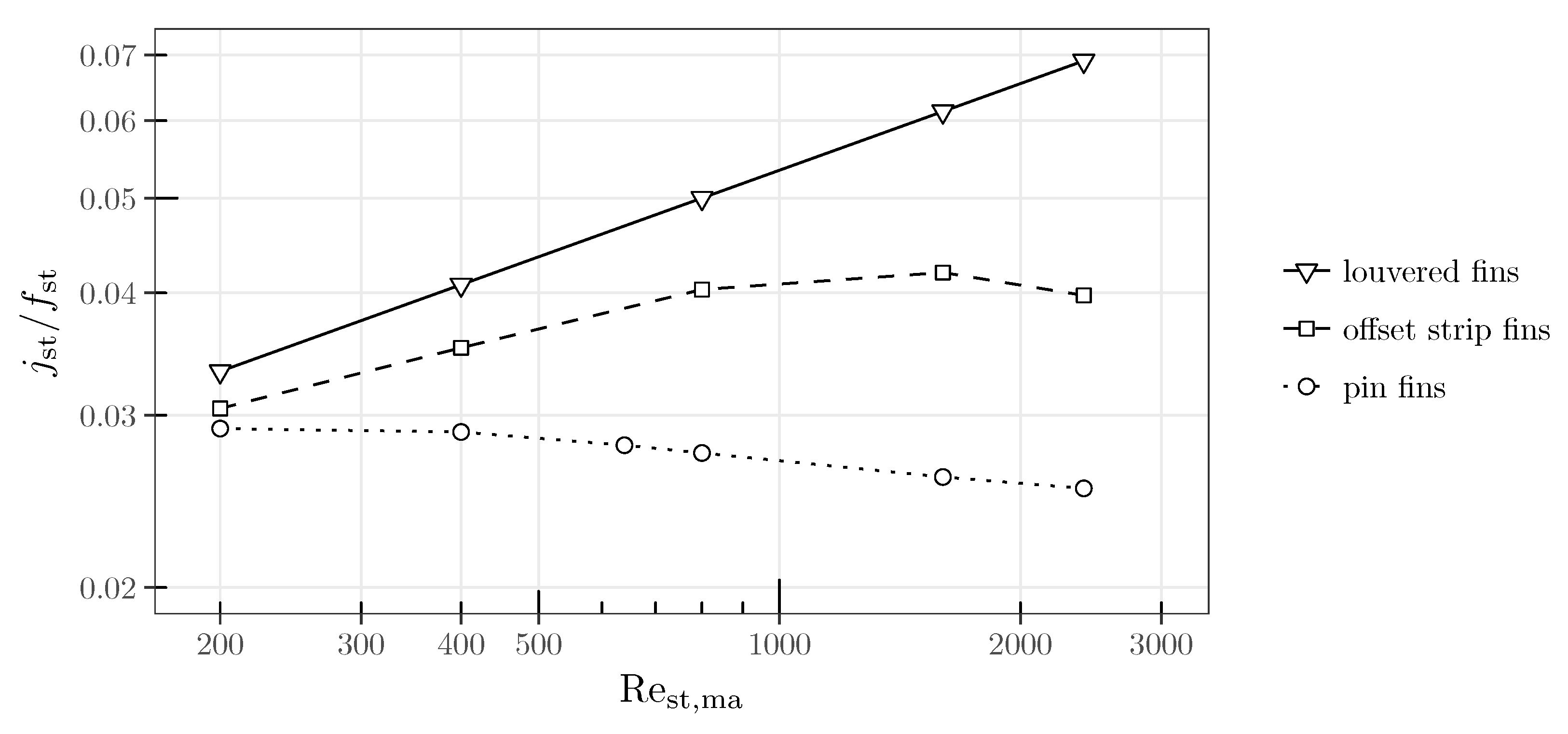
The first comparison is based on the area goodness factor $j_{\mathrm{st}}/f_{\mathrm{st}}$ ([5], p. 705) and it is shown in Figure 4. The louvered fins and the offset strip fins show slightly higher values for lower Reynolds numbers and much higher values for higher Reynolds numbers than the pin fins. The benefit of a high convective heat transfer in relation to viscous dissipation shrinks due to limitations in heat conduction through the fins (wire structure) and low surface area density (louvered fins, offset strip fins). These drawbacks cannot be accounted for, with the area goodness factor show in Figure 4, but will be addressed next.

Figure 4. Ratio of Colburn factor $j_{\mathrm{st}}$ and Fanning friction factor $f_{\mathrm{st}}$ versus Reynolds number for different enhancements.

Figure 5 shows the energy efficiency ${ϵ}_{\mathrm{E}}^{*}$ (cf. Table 3) for the three heat exchangers. The evaluation contains the limitation due to heat conduction through the fins and the surface area density. Thus, the offset strip fins and the pin fins show a better performance than in Figure 4. The energy efficiency is not necessarily increasing with Reynolds number. A decreasing fin efficiency and a flattening of the Nusselt number curve with increasing Reynolds number dampen the gradient. In particular, the wire structure shows this behaviour. The surface efficiency ${\eta }_0$ of the wire structures ranges from 0.72 for higher velocities to 0.8 for lower velocities. Thus, heat conduction through the structure already limits overall heat transfer considerably. For larger Reynolds numbers, the energy efficiency decreases for the offset strip and louvered fins (not visible) with respect to Reynolds number as well. For lower Reynolds numbers, the wire structures show a superior performance. From ${\mathrm{Re}}_{\mathrm{st},\mathrm{ma}}=550$ onwards, the louvered fins show the best performance.

Figure 5. Non-dimensional energy efficiency ${ϵ}_{\mathrm{E}}^{*}$ versus Reynolds number ${\mathrm{Re}}_{\mathrm{st},\mathrm{ma}}$ for different enhancements; standard comparison is at equal Reynolds numbers; grey dash-dot lines represent combinations of ${ϵ}_E^{*}$ and ${\mathrm{Re}}_{\mathrm{st},\mathrm{ma}}$ with equal $\dot{Q}/P_{\mathrm{diss}}$.

A huge advantage of this depiction is the well-defined range of energy efficiency values between 0.15 and 0.45 (in this example evaluation). A comparison at equal Reynolds numbers (and thus equal structure free-flow areas as described in Equation (12)) is very clear. Exemplarily, a comparison at ${\mathrm{Re}}_{\mathrm{st},\mathrm{ma}}=1600$ is shown by a vertical grey line in Figure 5. The louvered fins (marked with 1) show an efficiency 1.3 times higher than that of offset strip fins (2), and 1.5 times higher than that of pin fins (3). By implication, the pin fins will cause 1.5 times more dissipated power $P_{\mathrm{diss}}$ than the louvered fins for the same heat transfer rate $\dot{Q}$.

A comparison of the enhancement performance at different Reynolds numbers (cf. Equation (14)) has to consider the lines of equal heat transfer rate per dissipated power (grey dash-dot lines). A lower Reynolds number allows a lower energy efficiency. Thus, the louvered fins, operated at a Reynolds number shown by Point 4 in Figure 5 have the same ratio of $\dot{Q}/P_{\mathrm{diss}}$ as the offset strip fins operated at point 5 and the pin fins operated at point 6. One drawback is the need of a higher frontal structure area for lower Reynolds numbers (cf. Equation (12)). Another drawback will become clear when considering the volume or mass efficiency later on for lower Reynolds numbers. From the perspective of energy efficiency, lower velocities are preferable. Higher values of $\dot{Q}/P_{\mathrm{diss}}$ can be achieved for lower Reynolds numbers and/or higher non-dimensional energy efficiency ${ϵ}_{\mathrm{E}}^{*}$ (top left corner).

As a hypothesis on the mechanism of heat transfer and shear stress, the Reynolds Analogy (see e.g., [21]) supports reducing the velocity for higher values of $\dot{Q}/P_{\mathrm{diss}}$. The Analogy states that the Stanton number ($\mathrm{Nu}/$RePr) equals half the skin friction coefficient ($c_f/2$) at a Prandtl number of unity. Simplifications, such as neglecting form drag within the heat exchanger and extending the range of Prandtl numbers to values below, but close to unity (cf. [22]), yield a proportionality between the Nusselt number and the friction factor: $\mathrm{Nu}\propto f\mathrm{Re}$ (for constant Prandtl number). Thus, the energy efficiency ${ϵ}_{\mathrm{E}}^{*}$ is approximately constant for varying Reynolds numbers and $\dot{Q}$/$P_{\mathrm{diss}}$ is proportional to 1/$v_{\mathrm{st}}^2$ (more precise to 1/$\mathrm{Br}$). Thus, an increase in $\dot{Q}$/$P_{\mathrm{diss}}$ for lower Re_st,ma is not necessarily a consequence of a good enhancement structure and should not be misjudged.

Figure 6 shows a performance evaluation based on the volume needed for the enhancement structure. The wire structure shows a high potential. Along all Reynolds numbers, it shows more than twice the volume efficiency ${ϵ}_{\mathrm{V}}^{*}$. All curves have a negative slope. This is related to the definition of ${ϵ}_{\mathrm{V}}^{*}$ with the square of velocity $v_{\mathrm{st}}^2$ in the denominator in order to achieve a non-dimensional parameter independent of the hydraulic length. A comparison at equal Reynolds numbers is as straightforward as in Figure 5. A comparison at different Reynolds numbers needs a depiction of lines of equal $\dot{Q}/V_{\mathrm{st}}$. These lines have a negative slope as well. However, the gradient is steeper than that of the performance curves. Thus, higher Reynolds numbers allow higher values of $\dot{Q}/V_{\mathrm{st}}$ for the same enhancement structure.

Figure 6. Non-dimensional volume efficiency ${ϵ}_{\mathrm{V}}^{*}$ versus Reynolds number ${\mathrm{Re}}_{\mathrm{st},\mathrm{ma}}$ for different enhancements; standard comparison is at equal Reynolds number; grey dash-dot lines represent combinations of ${ϵ}_{\mathrm{V}}^{*}$ and ${\mathrm{Re}}_{\mathrm{st},\mathrm{ma}}$ with equal $\dot{Q}/V_{\mathrm{st}}$

Lastly, Figure 7 shows the mass efficiency ${ϵ}_{\mathrm{M}}^{*}$. The basic behaviour is similar to that in Figure 6 due to the same structure material density ${\rho }_{\mathrm{st}}$ and similar porosity ${\phi }_{\mathrm{st}}$.

Figure 7. Non-dimensional mass efficiency ${ϵ}_{\mathrm{M}}^{*}$ versus Reynolds number ${\mathrm{Re}}_{\mathrm{st},\mathrm{ma}}$ for different enhancements; standard comparison is at equal Reynolds numbers; grey dash-dot lines represent combinations of ${ϵ}_{\mathrm{M}}^{*}$ and ${\mathrm{Re}}_{\mathrm{st},\mathrm{ma}}$ with equal $\dot{Q}/m_{\mathrm{st}}$.

In Figure 8, the energy and the volume efficiencies are combined in one diagram. It shows the Pareto optimal sets [13] (or Pareto frontiers) at three different Reynolds numbers. For each of these Reynolds numbers, none of the three enhancements is superior to the others in both ${ϵ}_{\mathrm{E}}^{*}$ and ${ϵ}_{\mathrm{V}}^{*}$; with an increase in energy efficiency, a decrease in volume efficiency follows. The pin fins show, in each set, the highest volume efficiency; the louvered fins show the highest energy efficiency. However, the feasible set $\Theta$, the set of all possible points of the optimization problem, consists in this example solely of three feasible decision $\theta$ (three geometrically specified enhancements). In general, a larger feasible set with different enhancements and their geometric variations would be considered. A posteriori methods, such as evolutionary algorithms [13], could then be used to generate a new Pareto optimal set.

Figure 8. Pareto front of the bi-objective problem to optimize energy and volume efficiency. Fronts are given for three Reynolds numbers with three different enhancements in the feasible set $\Theta$.

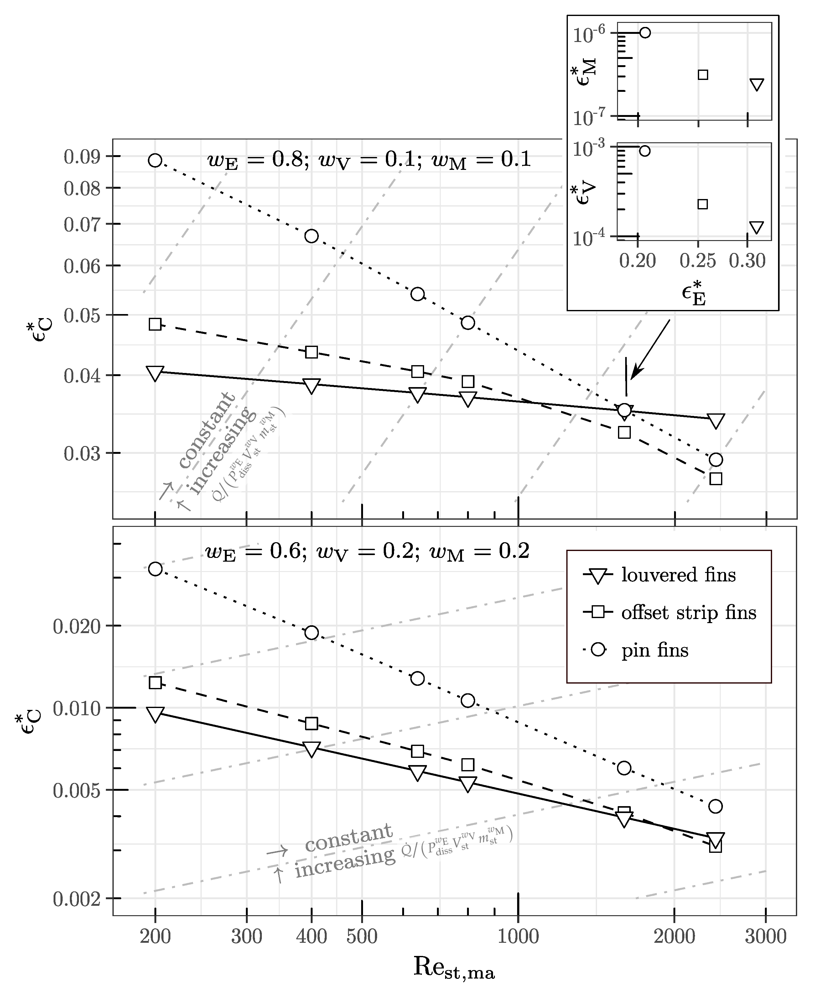
The combined ${ϵ}_{\mathrm{C}}$ efficiency is given in Figure 9. Two different sets of weighting factors were used exemplarily. The first set emphasizes the importance of the energy efficiency: with $w_{\mathrm{E}}=0.8$, $w_{\mathrm{V}}=0.1$, and $w_{\mathrm{M}}=0.1$, a change in energy efficiency by a factor $\zeta$ could be compensated by a change in volume efficiency by a factor ${\zeta }^{-8}$ (keeping the mass efficiency equal). This weighting yields a superior performance for the pin fins up to a Reynolds number of ${\mathrm{Re}}_{\mathrm{st},\mathrm{ma}}=1600$, compared to ${\mathrm{Re}}_{\mathrm{st},\mathrm{ma}}=550$ for the energy efficiency only (cf. Figure 5). The second set reduces the importance of the energy efficiency further on to $w_{\mathrm{E}}=0.6$, $w_{\mathrm{V}}=0.2$, and $w_{\mathrm{M}}=0.2$. In Figure 9 (bottom), the louvered fins show now the lowest performance for Reynolds numbers up to ${\mathrm{Re}}_{\mathrm{st},\mathrm{ma}}=2000$, compared to ${\mathrm{Re}}_{\mathrm{st},\mathrm{ma}}=550$ for the energy efficiency only (cf. Figure 5). These two weighing sets can serve as an example of an abundance of possible and reasonable weighting sets dependent on the application.

Figure 9. Combined efficiency ${ϵ}_{\mathrm{C}}^{*}$ versus Reynolds number ${\mathrm{Re}}_{\mathrm{st},\mathrm{ma}}$ for different enhancements; grey dash-dot lines represent combinations of ${ϵ}_{\mathrm{C}}^{*}$ and ${\mathrm{Re}}_{\mathrm{st},\mathrm{ma}}$ with equal $\dot{Q}/\left(P_{\mathrm{diss}}^{w_{\mathrm{E}}}{V}_{\mathrm{st}}^{w_{\mathrm{V}}}{m}_{\mathrm{st}}^{w_{\mathrm{M}}}\right)$; for ${\mathrm{Re}}_{\mathrm{st},\mathrm{ma}}=1600$, the data points are additionally shown in an ${ϵ}_{\mathrm{E}}^{*}$-${ϵ}_{\mathrm{V}}^{*}$ and ${ϵ}_{\mathrm{E}}^{*}$-${ϵ}_{\mathrm{M}}^{*}$ diagram similar to Figure 8.

4. Discussion

The introduction of the dimensional performance figures in Table 2, representing the ratio of the driving-force-specific heat transfer rate $\dot{Q}/\Delta T_{\mathrm{m}}$ to the dissipated power $P_{\mathrm{diss}}$, volume $V_{\mathrm{st}}$, and mass $m_{\mathrm{st}}$ is straightforward. The method uses the definition of efficiency in terms of benefit versus cost for all three types of costs analogously. The comprehensibility should be high; however, the drawback of a dependency on material properties is inevitable. For measurement, simulation, or correlation data for a specific application, this method can be sufficient for comparing different enhancements. A transfer to other operating conditions should be done with caution.

The transformation from the dimensional performance figures into non-dimensional figures considers driving parameters such as the Brinkman number for the energy efficiency. The driving parameters are expected to be equal for a comparison of different enhancements. This limitation of the comparison method is non-restrictive as long as the comparison is based on equal fluid free-flow areas $A_{\mathrm{in},\mathrm{st}}$ (and equal heat transfer rates).

When allowing different $A_{\mathrm{in},\mathrm{st}}$, relationships between ${\mathrm{Re}}_{\mathrm{st},\mathrm{ma}}$ and ${ϵ}^{*}$ are developed. These relationships can be integrated into the graphical visualization of the performance figures in a simple way. Thus, the restrictions are less strong (cf. restrictions (1) to (5)). An increase in $A_{\mathrm{in},\mathrm{st}}$ is usually needed in order to obtain the required fluid flow rate without an increase in the pressure drop and without a change in the heat exchanger volume [9]. It yields a reduced heat exchanger flow length. The shape is characteristic of heat exchangers in automotive and air conditioning applications. However, further increases in frontal areas are limited in these applications also by space availability. Thus, the need for more compact and lightweight heat exchangers remains in force.

The advantage of the proposed performance evaluation method is that different necessities can be considered separately with ${ϵ}_{\mathrm{E}}^{*}$, ${ϵ}_{\mathrm{V}}^{*}$, and ${ϵ}_{\mathrm{M}}^{*}$, as well as combined with ${ϵ}_{\mathrm{C}}^{*}$. The curves of ${ϵ}_{\mathrm{E}}^{*}$ in Figure 5 show distinct differences in performance with respect to the Reynolds number. The wire structures profit from high heat transfer coefficients, but yield high fluid friction. For higher Reynolds numbers, the fluid friction outweighs the beneficial heat transfer characteristics, such that ${ϵ}_{\mathrm{E}}^{*}$ shows lower values for the wire structure than for the louvered and strip fins. The effect of different Reynolds numbers on the volume and mass efficiency is less pronounced. The performance curves in Figure 6 and Figure 7 run approximately parallel to each other and with slightly less decrease than the lines of constant $\dot{Q}/V_{\mathrm{st}}$ and $\dot{Q}/m_{\mathrm{st}}$. Thus, the graphical visualization gives a clear indication of the performance with the wire structure, which has more than twice the volume and mass efficiency compared to the other two enhancements.

The method allows finding solutions to the multi-objective optimization problem $max\left({ϵ}_{\mathrm{E}}^{*}\left(\theta \right),{ϵ}_{\mathrm{V}}^{*}\left(\theta \right),{ϵ}_{\mathrm{M}}^{*}\left(\theta \right)\right)$ with $\theta \in \Theta$. Therein, the set $\Theta$ is the feasible set of decision vectors. In the exemplary enhancement comparison, $\Theta$ is composed of the louvered fins, the offset strip fins, and the wire structure. In a more general comparison, the feasible set should allow different geometrical parameters for each enhancement, such that the Pareto fronts in Figure 8 are shifted further to the top right corner for each enhancement type.

The combination of the efficiencies into ${ϵ}_{\mathrm{C}}^{*}$ allows for single-objective optimization. This scalarizing of the multi-objective optimization problem allows depicting optimal single-objective solutions that are equal to the Pareto optimal solutions of the multi-objective optimization problem.

5. Conclusions

Within this study, we have made the following achievements:

• Development of a dimensional performance evaluation method including energy, volume, and mass, allowing straightforward transfer to important quantities for real dimensioning,
• Transformation of dimensional performance evaluation quantities into non-dimensional quantities (efficiencies) based on comparable driving parameters,
• Application of the performance evaluation method to optimize a surface enhancement geometry (topology) or to compare different surface enhancements with each other,
• Control of energy, volume, and mass use for the optimization/comparison by setting the efficiencies as objective functions,
• Usage of thermal-hydraulic correlations from the literature, measurement data, or simulation data within the performance evaluation method,
• Development of a combined efficiency for single-objective optimization,
• Non-dimensional performance evaluation quantities are independent of characteristic lengths

Appendix E.1. Louvered Fins

The louvered fin geometry and performance correlation are taken from Kim et al. [15]. The geometry is shown in Figure A1; the detailed definitions of parameter values are given in Table A2.

Figure A1. Definition of geometrical parameters for a multi-louvered fin heat exchanger [15].

Table A2. Geometrical parameters of the louvered fin heat exchanger with nomenclature from [15] and nomenclature used within this study

Parameter Definition in [15]	Parameter Definition in This Study	Dimension	Value
$F_{\mathrm{p}}$	$l_{\mathrm{lateral}}$	mm	2.29
$L_{\mathrm{p}}$	$l_{\mathrm{longitudinal}}$	mm	4.76
${\delta }_{\mathrm{f}}$	$d_{\mathrm{st}}$	μm	152
$F_{\mathrm{d}}$	$L_{\mathrm{st}}$	mm	48
H	$H_{\mathrm{st}}$	mm	10
$L_{\mathrm{l}}$	‒	mm	9
$L_{\alpha }$	‒	${}^{\circ }$	28
$T_{\mathrm{p}}$	‒	mm	12

Table A2. Geometrical parameters of the louvered fin heat exchanger with nomenclature from [15] and nomenclature used within this study

Parameter Definition in [15]	Parameter Definition in This Study	Dimension	Value
$F_{\mathrm{p}}$	$l_{\mathrm{lateral}}$	mm	2.29
$L_{\mathrm{p}}$	$l_{\mathrm{longitudinal}}$	mm	4.76
${\delta }_{\mathrm{f}}$	$d_{\mathrm{st}}$	μm	152
$F_{\mathrm{d}}$	$L_{\mathrm{st}}$	mm	48
H	$H_{\mathrm{st}}$	mm	10
$L_{\mathrm{l}}$	‒	mm	9
$L_{\alpha }$	‒	${}^{\circ }$	28
$T_{\mathrm{p}}$	‒	mm	12

Appendix E.2. Offset Strip Fins

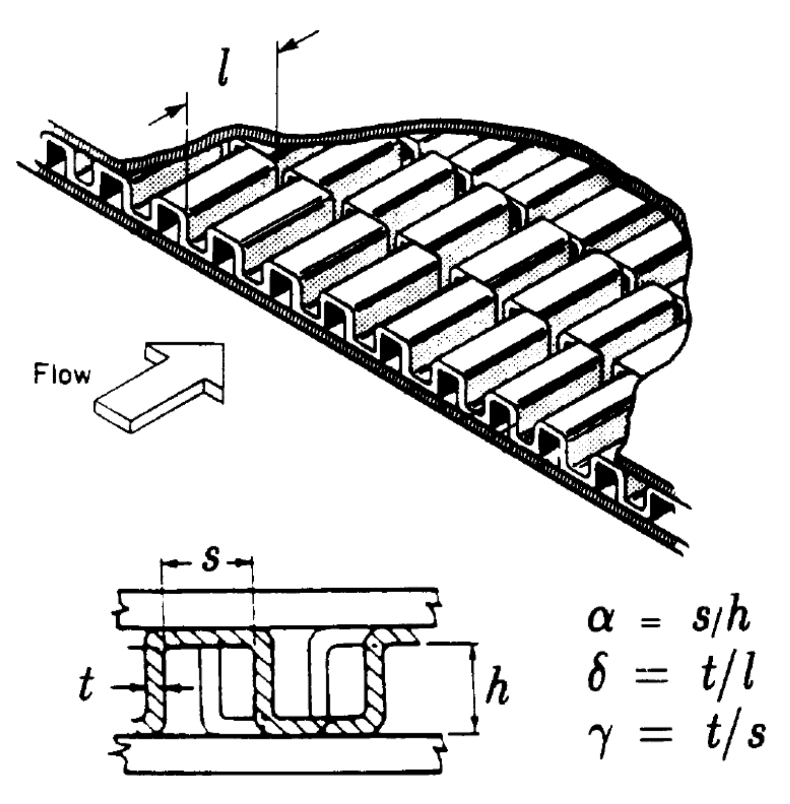
The offset strip fin geometry and performance correlation are taken from Manglik et al. [16]. The geometry is shown in Figure A2; the detailed definitions of parameter values are given in Table A3.

Figure A2. Definition of geometrical parameters for an offset strip fin heat exchanger [16].

Table A3. Geometrical parameters of the offset strip fin heat exchanger with nomenclature from [16] and nomenclature used within this study

Parameter Definition in [16]	Parameter Definition in This Study	Dimension	Value
$s+t$	$l_{\mathrm{lateral}}$	mm	1.9
l	$l_{\mathrm{longitudinal}}$	mm	1.01
t	$d_{\mathrm{st}}$	μm	152
$h+t$	$H_{\mathrm{st}}$	mm	10

Table A3. Geometrical parameters of the offset strip fin heat exchanger with nomenclature from [16] and nomenclature used within this study

Parameter Definition in [16]	Parameter Definition in This Study	Dimension	Value
$s+t$	$l_{\mathrm{lateral}}$	mm	1.9
l	$l_{\mathrm{longitudinal}}$	mm	1.01
t	$d_{\mathrm{st}}$	μm	152
$h+t$	$H_{\mathrm{st}}$	mm	10

Appendix E.3. Wire Structure Pin Fins

The wire structure pin fin geometry and performance correlation are taken from Fugmann et al. [17]. The geometry is shown in Figure A3.

Figure A3. Definition of geometrical parameters for a wire structure pin fin heat exchanger [17].

References

- Stone, K.M. Review of Literature on Heat Transfer Enhancement in Compact Heat Exchangers; Air Conditioning & Refrigeration Center: Urbana, IL, USA, 1996. [Google Scholar]
- Fugmann, H.; Laurenz, E.; Schnabel, L. Wire Structure Heat Exchangers—New Designs for Efficient Heat Transfer. Energies 2017, 10, 1341. [Google Scholar] [CrossRef]
- LaHaye, P.G.; Neugebauer, F.J.; Sakhuja, R.K. A Generalized Prediction of Heat Transfer Surfaces. J. Heat Transf. 1974, 96, 511. [Google Scholar] [CrossRef]
- Webb, R.L. Goodness Factor Comparisons. In HEDH Multimedia; Begellhouse: Danbury, CT, USA, 2014. [Google Scholar] [CrossRef]
- Shah, R.K.; Sekulić, D.P. Fundamentals of Heat Exchanger Design, 1st ed.; John Wiley & Sons: Hoboken, NJ, USA, 2003. [Google Scholar]
- Webb, R.L.; Kim, N.H. Principle of Enhanced Heat Transfer; Taylor & Francis: Abingdon, UK, 1994. [Google Scholar]
- Soland, J.G. Performance Ranking of Plate-Finned Heat Exchanger Surfaces. Ph.D Thesis, Massachusetts Institute of Technology, Cambridge, MA, USA, 1975. [Google Scholar]
- Cowell, T.A. Comparison of Compact Heat Transfer Surfaces. J. Heat Transf. 1990, 112, 288–294. [Google Scholar] [CrossRef]
- Sahiti, N.; Durst, F.; Dewan, A. Strategy for selection of elements for heat transfer enhancement. Int. J. Heat Mass Transf. 2006, 49, 3392–3400. [Google Scholar] [CrossRef]
- Li, Q.; Flamant, G.; Yuan, X.; Neveu, P.; Luo, L. Compact heat exchangers: A review and future applications for a new generation of high temperature solar receivers. Renew. Sustain. Energy Rev. 2011, 15, 4855–4875. [Google Scholar] [CrossRef]
- Marthinuss, J.E. Air Cooled Compact Heat Exchanger Design For Electronics Cooling. Coolers Design Heat Sinks Test Measur. 2004, 10, 28. [Google Scholar]
- Korhonen, P.; Wallenius, J. Visualization. In Multiple Objective Decision-Making Framework; Springer: Berlin, Germany, 2008. [Google Scholar]
- Miettinen, K.; Mäkelä, M.M. On scalarizing functions in multiobjective optimization. OR Spectr. 2001, 24, 193–213. [Google Scholar] [CrossRef]
- Triantaphyllou, E.; Parlos, P.M. Multi-Criteria Decision Making Methods: A Comparative Study. In Applied Optimization; Kluwer Academic Publishers: Dordrecht, The Netherlands, 2010; Volume 44. [Google Scholar]
- Kim, M.H.; Bullard, C.W. Air-side thermal hydraulic performance of multi-louvered fin aluminum heat exchangers. Int. J. Refrig. 2002, 25, 390–400. [Google Scholar] [CrossRef]
- Manglik, R.M.; Bergles, A.E. Heat transfer and pressure drop correlations for the rectangular offset strip fin compact heat exchanger. Exp. Therm. Fluid Sci. 1995, 10, 171–180, Figures reprinted with permission from Elsevier. [Google Scholar] [CrossRef]
- Fugmann, H.; Schnabel, L.; Frohnapfel, B. Heat Transfer and Pressure Drop Correlations for Laminar Flow in an In-line and Staggered Array of Circular Cylinders. Numer. Heat Transf. Part A Appl. 2019, 75, 1–20. [Google Scholar] [CrossRef]
- Fugmann, H.; Di Lauro, P.; Sawant, A.; Schnabel, L. Development of Heat Transfer Surface Area Enhancements: A Test Facility for New Heat Exchanger Designs. Energies 2018, 11, 1322. [Google Scholar] [CrossRef]
- Dong, J.; Chen, J.; Chen, Z.; Zhang, W.; Zhou, Y. Heat transfer and pressure drop correlations for the multi-louvered fin compact heat exchangers. Energy Convers. Manag. 2007, 48, 1506–1515, Figures reprinted with permission from Elsevier. [Google Scholar] [CrossRef]
- Dong, J.; Chen, J.; Chen, Z.; Zhou, Y. Air-side thermal hydraulic performance of offset strip fin aluminum heat exchangers. Appl. Therm. Eng. 2007, 27, 306–313. [Google Scholar] [CrossRef]
- Mahulikar, S.P.; Herwig, H. Fluid friction in incompressible laminar convection: Reynolds’ analogy revisited for variable fluid properties. Eur. Phys. J. B 2008, 62, 77–86. [Google Scholar] [CrossRef]
- MIT. The Reynolds Analogy. 2019. Available online: web.mit.edu.
- Böckh, P.; Wetzel, T. Wärmeübertragung: Grundlagen und Praxis, Aktualisierte und Überarbeitete Auflage ed.; Lehrbuch Springer Vieweg: Berlin, Germany, 2017. [Google Scholar]
- Verein Deutscher Ingenieure. Wärmeatlas, 9th ed.; Springer: Berlin/Heidelberg, Germany, 2002. [Google Scholar]
Figure 1.
Dimensional (a) and non-dimensional (b) energy efficiency and , respectively, versus Reynolds number for a fully developed laminar and turbulent flow in a smooth circular tube and a rectangular duct; air is used in (a) as fluid at 25 and 1 atm with a hydraulic diameter of 5 ; the transition flow is not shown. Data is based on [5].
Figure 2.
Scheme of a performance visualization generation for different types of heat transfer enhancements in differently sized heat exchangers.
Figure 3.
Geometry examples of a louvered fin [19], and offset strip fin [20], and a wire structure pin fin enhancement used for the visualization method.
Figure 4.
Ratio of Colburn factor and Fanning friction factor versus Reynolds number for different enhancements.
Figure 5.
Non-dimensional energy efficiency versus Reynolds number for different enhancements; standard comparison is at equal Reynolds numbers; grey dash-dot lines represent combinations of and with equal .
Figure 6.
Non-dimensional volume efficiency versus Reynolds number for different enhancements; standard comparison is at equal Reynolds number; grey dash-dot lines represent combinations of and with equal
Figure 7.
Non-dimensional mass efficiency versus Reynolds number for different enhancements; standard comparison is at equal Reynolds numbers; grey dash-dot lines represent combinations of and with equal .
Figure 8.
Pareto front of the bi-objective problem to optimize energy and volume efficiency. Fronts are given for three Reynolds numbers with three different enhancements in the feasible set .
Figure 9.
Combined efficiency versus Reynolds number for different enhancements; grey dash-dot lines represent combinations of and with equal ; for , the data points are additionally shown in an - and - diagram similar to Figure 8.