Article

Innovative Control Strategies for the Diagnosis of Injector Performance in an Internal Combustion Engine via Turbocharger Speed

1
Department of Industrial Engineering (DIEF), Università degli Studi di Firenze, via di Santa Marta 3, 50139 Firenze, Italy
2
Yanmar R&D Europe, Viale Galileo 3/A, 50125 Firenze, Italy
3
Yanmar Co. Ltd., 1-32, Chayamachi, Kita-ku, Osaka-sh, Osaka 8308311, Japan
*
Author to whom correspondence should be addressed.
Energies 2019, 12(8), 1420; https://doi.org/10.3390/en12081420
Submission received: 21 March 2019 / Revised: 4 April 2019 / Accepted: 9 April 2019 / Published: 12 April 2019
(This article belongs to the Special Issue Internal Combustion Engines 2018)

Abstract

:
In order to ensure a high level of performance and to comply with the increasingly severe limitations in terms of fuel consumption and pollution emissions, modern diesel engines need continuous monitoring of their operating conditions by their control units. With particular focus on turbocharged engines, which are presently the standard in a large number of applications, the use of the average and the instantaneous turbocharger speeds is thought to represent a valuable feedback of the engine behavior, especially for the identification of the cylinder-to-cylinder injection variations. The correct operation of the injectors and control of the injected fuel quantity allow the controller to ensure the right combustion process and maintain engine performance. In the present study, two different techniques are presented to fit this scope. The techniques are discussed and experimentally validated, leading to the definition of an integrated control strategy, which features the main benefits of the two, and is able to correctly detect the cylinder-to-cylinder injection variation and, consequently, properly correct the injection in each cylinder in order to balance the engine behavior. In addition, the possibility of detecting misfiring events was assessed.

1. Introduction

The reliability and efficiency of internal combustion engines make them the most applied technology solution throughout the world in multiple roles, such as transport, power generation, and industrial application. In order to guarantee a high level of performance and to comply with challenging new regulations, continuous supervision of engine operating conditions is needed (e.g., [1,2]), with particular reference to fuel consumption [3], combustion control [4], and pollution emissions [5,6]. To this end, the monitoring of the engine’s thermodynamic cycle is the most suitable approach. During the development stage of a new unit, direct analyses of the in-cylinder pressure are commonly performed at the test bench in order to optimize the engine’s thermodynamic cycle, with particular focus on the combustion process. Indeed, the in-cylinder pressure is one of the most important parameters for the analysis of combustion; however, its direct measurement using a pressure sensor is often intrusive and expensive. For this reason, many solutions of indirect measurements exploiting nonintrusive and low-cost sensors have been studied. The most diffused and studied monitoring methodologies are based on different types of acoustic emissions [7,8,9,10,11], vibration analysis [12,13,14,15], or crankshaft engine speed analysis [16,17,18,19,20,21].
The generation of noise in ICEs comes from aerodynamic and mechanical sources. The source of noise caused by air perturbation can be defined as an aerodynamic source, i.e., turbulence within the exhaust and intake system. Noise generated through contacts, impacts, and shocks between surfaces are the mechanical source, including, for example, impacts between cylinders and pistons, shafts, and supports, etc. Because of the above, several different contributions are included in the overall acoustic emissions from the engine; the difficulty of the isolation of each contribution within this emission represents one of the biggest issues related to engine condition monitoring based on acoustic emissions. The use of acoustic signals as a monitoring methodology is limited currently by the masking effect given by the background noise and preprocessing operations are mandatory to obtain a reliable signal [22].
The vibration method is often adopted for the detection and control of engine knocking in spark ignition engines. Diesel engines present four different sources of vibrations: combustion, piston slap, fuel injection valve operation, and inertial forces that move the engine block in its supports. Antoni et al. [23] pointed out that the majority of these sources of vibration are linked with events that occur in a small crank-angle window around the piston top-dead center. The consequent overlapping vibration signatures represent, in the analysis of the engine vibration signals, one of the most important problems. When a misfiring or a knock event take place, a complex vibration pattern is created. By analyzing this pattern, it is theoretically possible to detect in which cylinder(s) a malfunction is occurring. Vibrational measures, on the other hand, are affected by a low signal-to-noise ratio at low frequencies that influences the correct reconstruction of the engine cycle.
Techniques for condition monitoring of the ICE by means of the crank-angle measurements are based on the angular speed and acceleration fluctuation of the crankshaft. These fluctuations are linked to the fast variation of the in-cylinder pressure for each cylinder during engine operation. The measurements of the crankshaft speed variation could be used to evaluate both the engine torque and the in-cylinder pressure. Crank-angle-based monitoring techniques have many advantages, among which are the availability of already used crankshafts sensors, the low-cost of the sensors, the possibility to distinguish the contribution of each cylinder, and the nonintrusive nature of the measurement. However, one of the main disadvantages of these techniques is the poor sensitivity of the crankshaft speed, due to the high inertia of the engine, meaning that the fault has to be sufficiently severe to cause a variation in terms of the torque having a measurable effect on the crankshaft velocity fluctuation. Another weakness of these techniques is related to the inability of identifying specific component-related faults [24].
Monitoring strategies based on turbocharger (TC) speed are studied due to its strict connection with all the important parameters of a turbocharger diesel engine (TCDE) [25]. Many engine parameters can be detected, such as the EGR ratio, the fuel injection characteristics, the combustion process, or the environmental pressure, and it requires nonintrusive and inexpensive measurements. By monitoring the TC speed, faults regarding many engine conditions can be identified, including a different injection mass in one cylinder and in which cylinder this difference occurs [26,27,28]. However, the TC speed is not yet exploited to its full potential.
In this paper, considering the growing use of turbochargers (TC) in all modern compression ignited and spark ignited internal combustion engines, a detailed study on the use of the average and instantaneous TC speed as a feedback of the engine operating conditions is presented [29].
Two different approaches, based on time and frequency content of the TC speed are presented and compared numerically and experimentally for a four-stroke turbo-diesel engine, focusing on the possibility of monitoring the performance of the engine injectors. The two methodologies were initially theorized by some of the authors in [30,31] based on numerical simulations. In the present study, both approaches have been first made more systematic and robust (e.g., with a more detailed treatment of the experimental signal of the turbocharger speed). Then, a specific experimental campaign was carried out to verify the reliability of the two methodologies. In particular, two different sets of injectors were tested, one with a homogeneous performance among cylinders and a deteriorated one with a different performance for each cylinder. As an additional point of novelty, an integrated procedure able to combine the benefits of the two methodologies has been figured out, being easily implementable in real engines and able to detect misfiring events.

2. Developed Techniques to Monitor the Injector Performance Based on Turbocharger Speed

Upon examination of the sensitivity of the instantaneous TC speed to the cylinder-to-cylinder and to the global injection variation, two methodologies have been theoretically conceived in the recent past [30,31] with the aim of detecting the actual fuel quantity injected in each cylinder during engine operation. In previous studies, the methodologies were set up making use of a 1D numerical model of the same engine that was then tested in the present study. The two techniques are, respectively, based on:
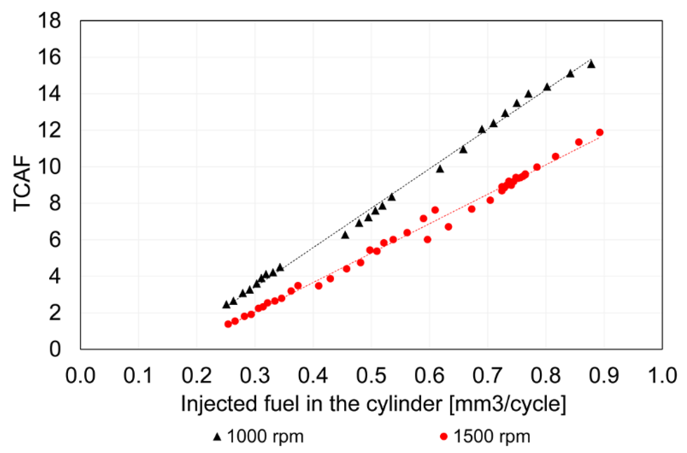
  • the acceleration of the turbocharger equal to the derivative of the TC speed signal
  • the frequency content of the TC speed signal analyzed by means of a Fast Fourier Transformation (FFT)
The two approaches are presented and discussed in the following section, pointing out their main benefits and drawbacks, while the following sections reports the results of the extensive experimental campaign that has been carried out for their validation and assessment.

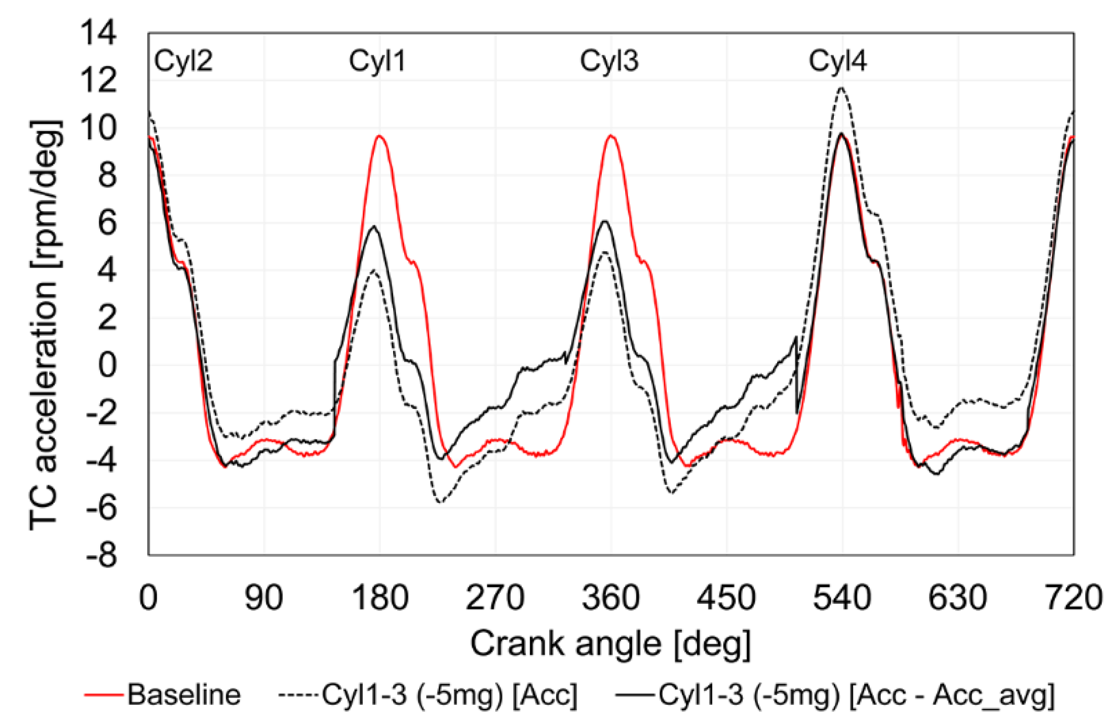
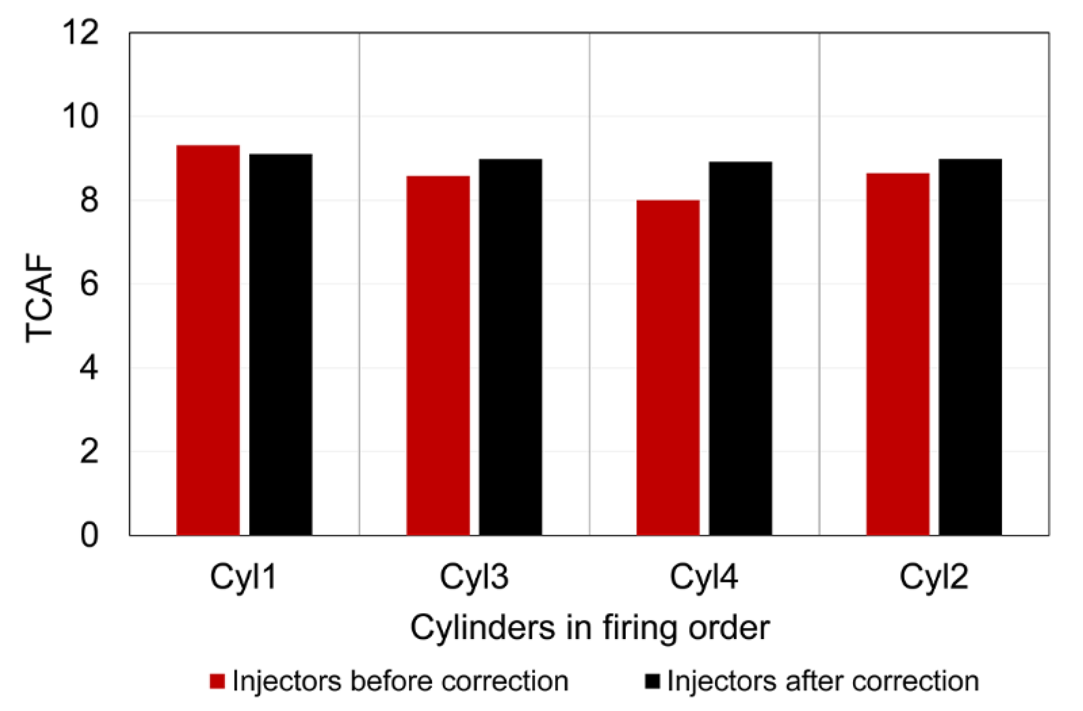
2.1. Technique Based on TC Acceleration

This technique makes use of TC acceleration information contained in the TC speed signal. The evolution of the TC speed during each engine cycle is directly influenced by the pressure waves coming from the discontinuous functioning of the internal combustion engine, which enter the turbine inlet. Since this pressure profile, in turn, depends on the engine combustion process and then to the fuel quantity injected in each cylinder, the TC acceleration is proposed for use as a parameter for the monitoring of the fuel injection. As a confirmation of the above, Figure 1 confirms good agreement between the TC acceleration and pressure waves at the engine outlet. Data in Figure 1 (and in the whole Section 2) come from numerical simulations on the same engine used in [29] carried out with the calibrated 1D model, but they are fully representative of the situation commonly found in engines during operation.
In order to correlate each cylinder to the corresponding acceleration peak, the whole engine cycle has to be divided into four crank-angle (CA) windows, in each of which, a cylinder gives the most relevant contribution to the instantaneous TC speed oscillation. To this end, the minimum value of the TC speed is considered as the end of the contribution of one cylinder. As soon as the TC speed starts increasing again, this new phase can be associated with the opening of the exhaust valve of the subsequent cylinder (in terms of firing order). In other words, the windows of influence are defined starting from the minimum value of the TC speed, dividing the remaining cycle into a number of equally-spaced windows having a CA duration obtained by dividing for the number of cylinders of the engine (e.g., 180° of CA in case of a four-cylinder engine).
In addition, in any window of influence, the acceleration signal is purged by the average acceleration within the window itself. This precaution is needed to avoid the analysis from being affected by the mutual influence among cylinders that can be represented by the average exhaust pressure.
The effects of this procedure are clearly distinguishable in Figure 2, where the instantaneous TC acceleration purged by the average value for each cylinder-window is compared to the actual acceleration and the baseline case. The results in Figure 2 (data derived from the model of [29]) are again obtained with the same 1D model used in Figure 1.
The resulting value in time was called TurboCharger Acceleration Factor (TCAF). To summarize, the TCAF (Equation (1)) is defined for each cylinder (Cyl_i) as the maximum acceleration value (acc) measured in its corresponding time window (in terms of CA degrees) reduced by the average calculated in the related contribution window (Equation (2)), where ω is the TC speed and ϑ is the CA (f and i are the final and initial instants of the window, respectively).
T C A F C y l _ i = a c c p e a k a c c a v g ϑ f , ϑ i .
a c c a v g ϑ f , ϑ i = ω T C ( ϑ f ) ω T C ( ϑ i ) ϑ f ϑ i .
By its nature, the TCAFCyl_i is related to the fuel quantity injected in the ith cylinder. The reliability of the acceleration methodology for the injector performance monitoring is, however, limited by the engine speed. In previous studies [30,31], it was shown in fact that at high engine rotational speeds (3000 rpm and above), the correlation between the TCAF parameter and the injected fuel in one of the cylinders is no longer stable and exploitable, due to the following reasons:
  • at high engine rotational speeds, the scavenging phase (if present) managed by the valve overlap makes the pressure wave coming from the inlet duct (i.e., from the compressor) affect the pressure at the turbine inlet and the instantaneous TC speed;
  • high engine speeds are connected to strong pressure pulsations, and consequently to instantaneous TC speed oscillations, characterized by very high frequency, as testified by Equation (3), where n c y l is the number of cylinders, N is the average engine speed and T is the number of strokes of the engine. This frequency is called firing frequency;
    f = 2   N   n c y l   T 1 .
  • since the turbine response is mostly affected by its inertia, the difference between the acceleration trend and the pressure oscillation increases with respect to lower regimes and the TCAF is not able to give useful information about the cylinder-to-cylinder injection variation.

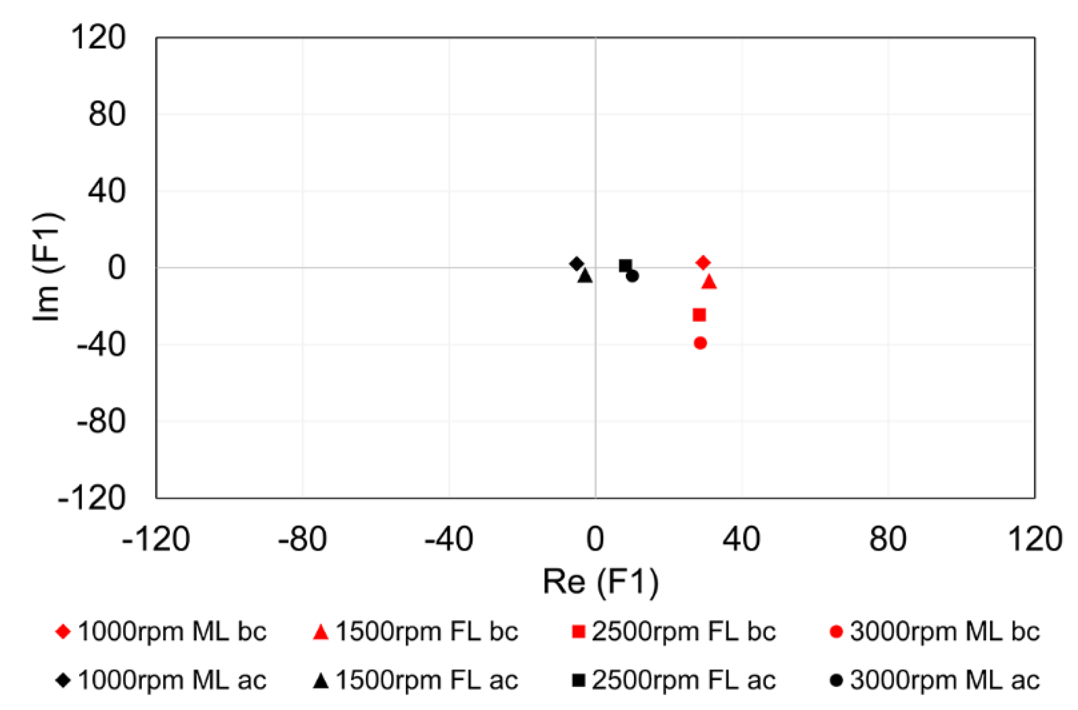
2.2. Frequency Content-Based Monitoring Technique

The second monitoring methodology is based on the analysis of the main orders of the turbocharger speed signal. Orders are commonly used in ICE analysis since they consider the frequency of an event in terms of equivalent crank angle; for example, the “first order” refers to an event that occurs once during each engine cycle, so that its frequency in time changes proportionally to the engine revolution speed. In this view, the use of orders allows one to assess easily a methodology and/or a phenomenon at different engine revolution speeds.
In the present case, if all injectors are able to supply the same fuel quantity in each cylinder, most of the engine working variables, such as the instantaneous speed of the crankshaft, the intake and exhaust dynamic pressure, and the instantaneous turbocharger speed, will be characterized by the same main frequency, i.e., the firing frequency.
The developed methodology makes use of different order in the engine functioning to get a complete representation of different phenomena. A brief description of each significant order used is reported following [30,31]:
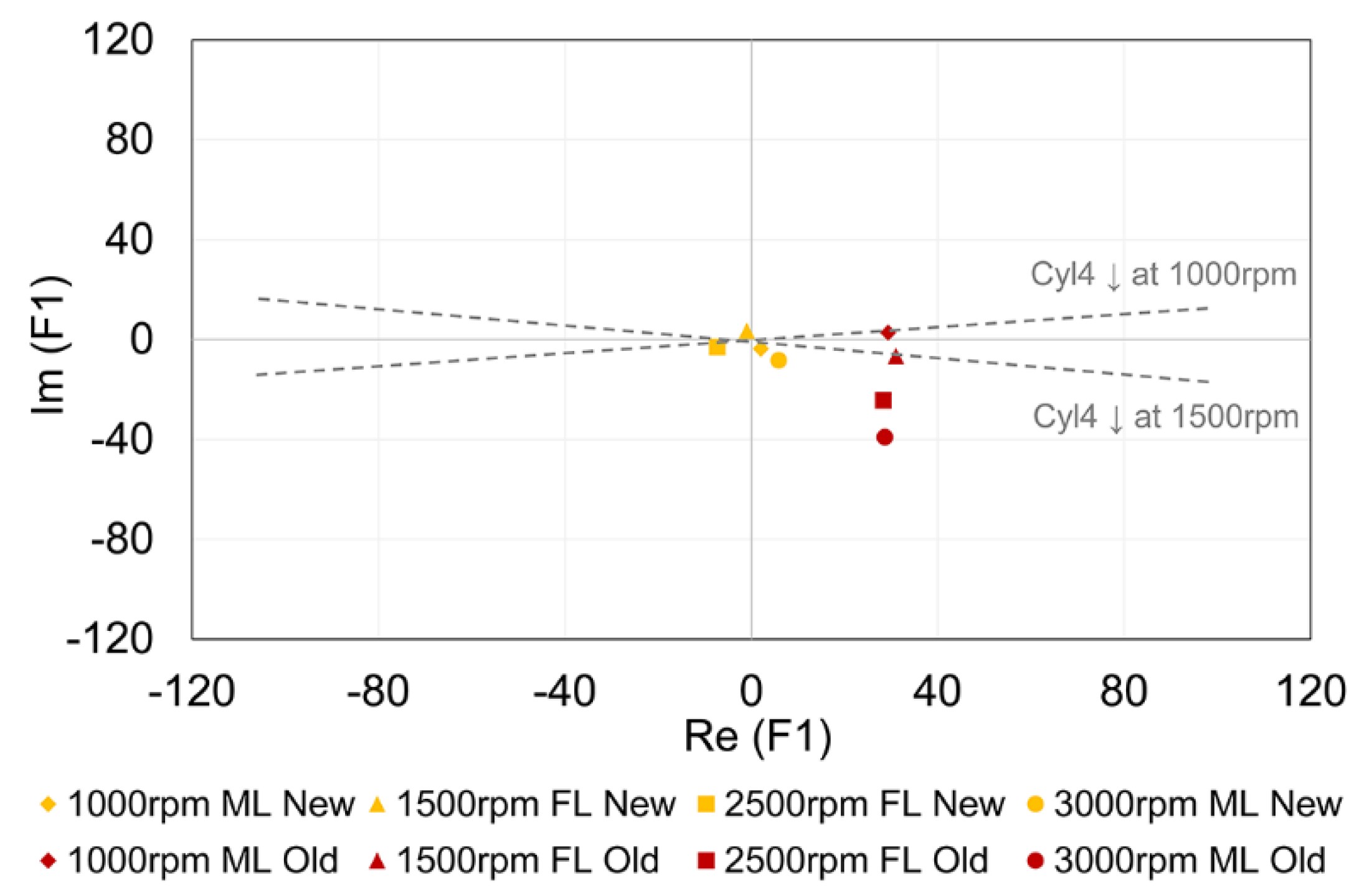
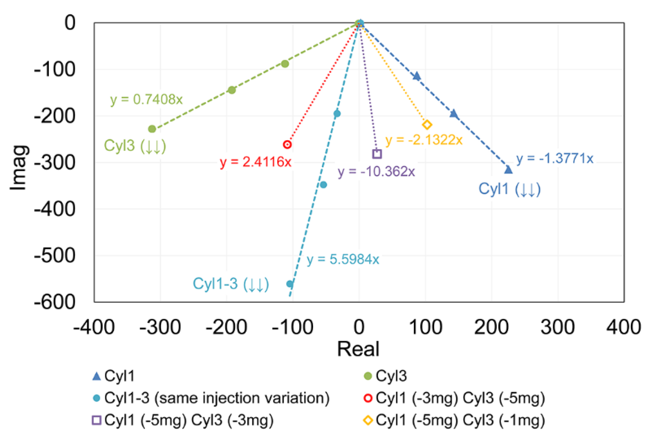
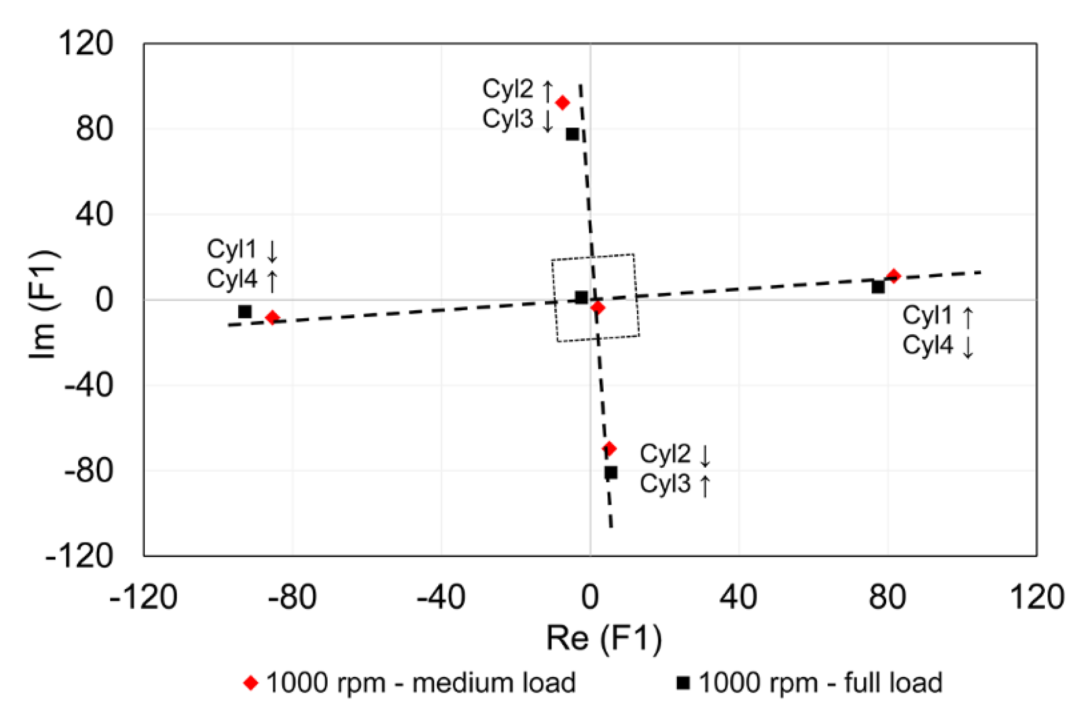
  • F1, first order corresponds to one event for each engine cycle. F1 will be dominant in the case of injection variation on one cylinder or in the case of an equal injection variation in two cylinders, which are consecutive in the firing order (1&3 or 2&4). F1 is defined in Equation (4).
    F 1 = 1 4   f = 1 2   N .
  • F2, second order corresponds to two events for each engine cycle. This order becomes dominant in the specific case in which there is an equal injection for nonconsecutive cylinders in the firing order (1&4 and 2&3).
  • F3, third order corresponds to three events for each engine cycle. It is not connected with a specific injection case.
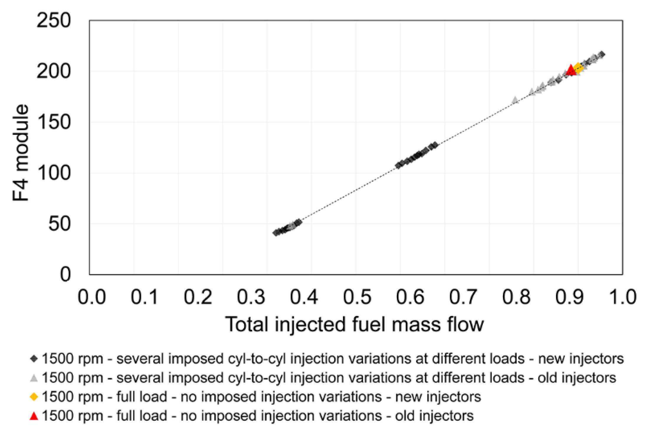
  • F4, fourth order corresponds to four events for each engine cycle. It represents the firing frequency (Equation (5)) and it is the dominant order in case of homogeneous injection.
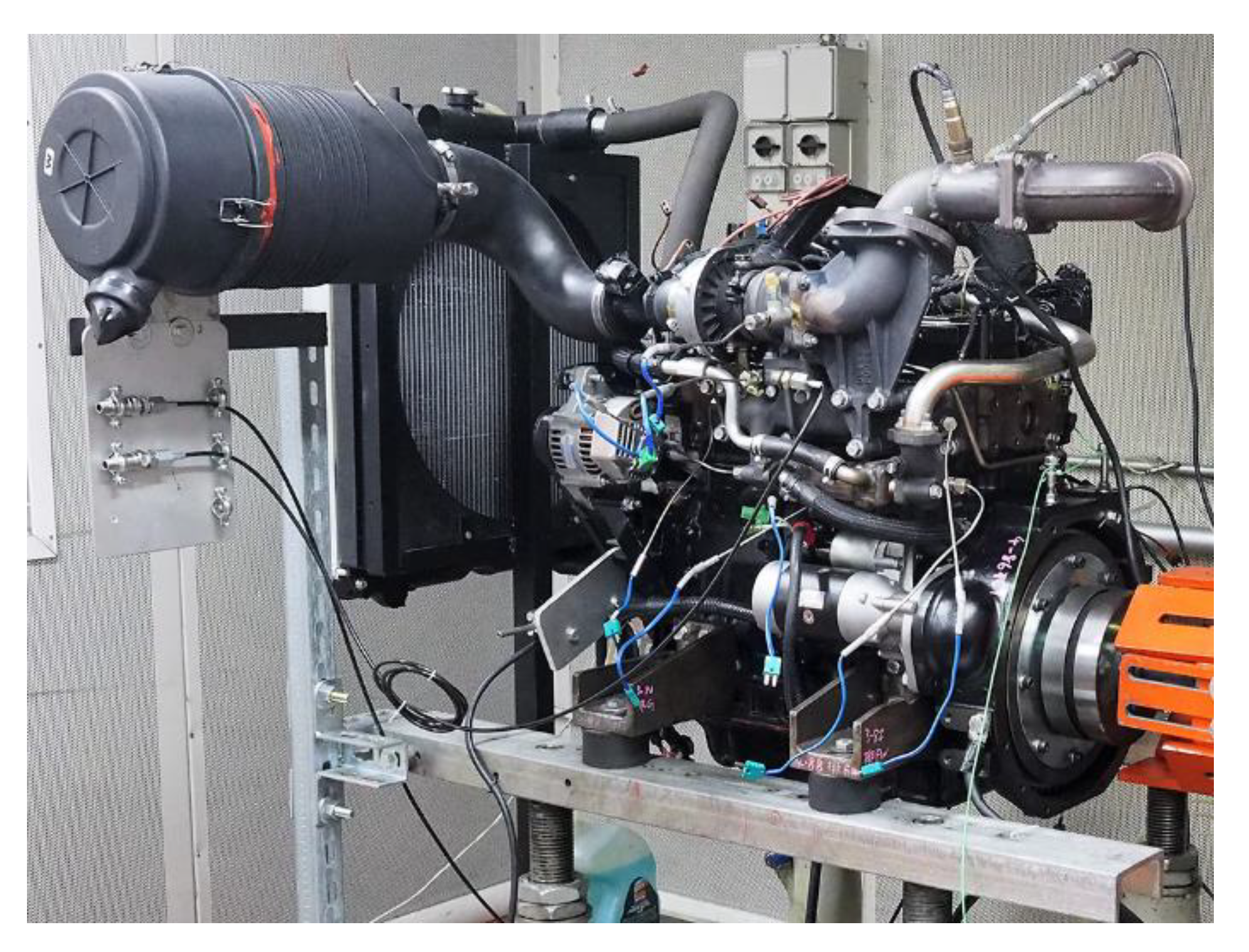
    F 4 = f = 2   N .
In particular, the module of the fourth order is associated with the base oscillation amplitude of the instantaneous turbocharger speed that in turn is directly linked to the total amount of injected fuel. Thus, the total injected fuel in the engine can be correlated linearly to the fourth order, also in case of strong variations of the engine load. The consideration above is true as long as the engine speed is kept constant. The coefficient of the linear proportionality does change, however, by varying the engine rotational speed, as discussed in [31]. Conversely, it is indeed true that the sensitivity on the F4 module grows by reducing the engine speed.
If, as discussed, the total injected fuel in the engine can be quantified upon analysis of the F4 module, the complex forms of the first (F1) and the second (F2) orders have to be taken into account in order to detect possible cylinder injection inhomogeneity, i.e., to analyze the frequency content of the TC speed signal.
The analysis procedure can be schematized as follows. First, the specific oscillation of the TC speed in each cylinder is characterized, i.e., the F1 phase is calculated. Indeed, if the cylinder under investigation is experiencing a different amount of fuel injected, a different F1 phase is about to be measured. Then, in order to quantify the injection variation and to distinguish whether there is an increase or a decrease in the injection, the F4 module is exploited. Moreover, it is possible to quantify the injection variation in case the injector fails in two cylinders; the distribution of the total variation among the cylinders can be reconstructed by the first order phase variation with respect to the characteristic phase of one of the cylinders affected by the injection variation.
As an illustrative example, Figure 3 and Table 1 report the results of the methodology related to different injection variations in cylinder 1 and cylinder 3 (data again taken from the 1D numerical model). As discussed, the fourth order module has been exploited to determine the total injection variation, while the first order phase allows one to identify the cylinder where the singularity takes place. In case the total injection variation involves two cylinders (consecutive in terms of firing order), the percentage variation of the phase with respect to the characteristic phase of cylinder 1, taken as the reference, is equal to the percentage distribution of the total fuel variation between the two cylinders.
In the case of injection variations in two nonconsecutive cylinders, the related first order phase does not change with respect to the characteristic phase of the cylinders affected by the injection variation. Thus, in order to detect this kind of variation, one can compare the module of the second order to that of the first one: when the F2 module is larger than that of F1, a variation in two nonconsecutive cylinders is expected.
The complete algorithm for the injector performance monitoring is reported in Figure 4.

3. Experiments

Extensive experimental investigation was carried out with the aim of: a) validating the two methodologies, and b) pointing out their specific benefits and drawbacks.

3.1. Experimental Layout

The experimental activity was performed on a YANMAR four-stroke, four-cylinder, turbo-diesel engine with a displacement of 2100 cm3 for heavy-duty application, whose main characteristics are reported in Table 2. The engine was installed at the test bench of the Department of Industrial Engineering (DIEF) of the University of Firenze (Italy), depicted in Figure 5.
The engine was completely instrumented in order to monitor the engine operating parameters. The measured signals can be divided into dynamic and static. A summary of the signals is reported in the following.
Dynamics signals:
  • in-cylinder pressure in all the cylinders
    Piezoelectric sensor Kistler 6125C11
    Max pressure 300 bar
  • pressure in the exhaust manifold upstream the turbine
    Piezoresistive sensor Kulite EWCT-312M, air cooled
    Max pressure 3.5 barA
  • injection phasing
    Chauvin Arnoux E3N Current clamp
    Operating range: 50 to 100 mA
  • crankshaft angular position and TDC reference
    optical Encoder AVL 365C
    Angular resolution 0.5°
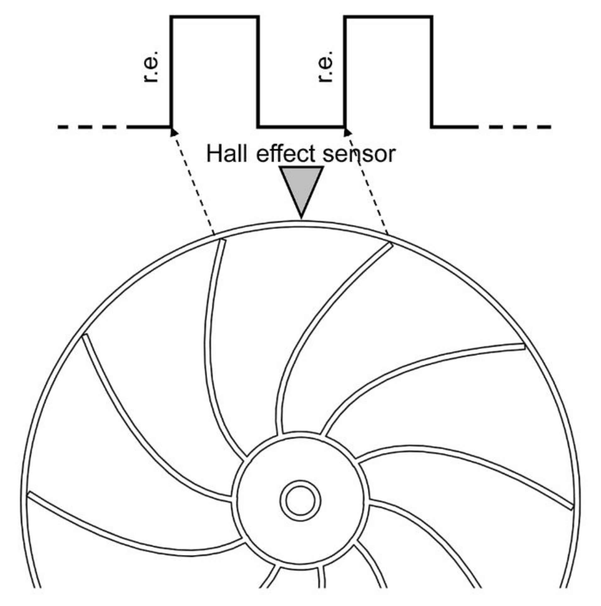
  • compressor blade passage (turbocharger speed)
    AEC turbo speed unit SF-030
    blade number from 8 to 20
    max speed 150000 rpm (20 blades) / 400000 rpm (8 blades)
The temperature of the exhaust line was measured by means of K-type thermocouples installed with a dedicated connector, while T-type thermocouples were used along the intake line. All static pressure values were measured by Gems pressure sensor, model 3500, with an operating range of 0–5 bar and an accuracy of 0.25% of FS.
  • torque and power of the engine
  • exhaust temperature of each cylinder
  • temperature and pressure at the compressor inlet
  • temperature and pressure at the compressor outlet
  • temperature and pressure at the turbine inlet
  • temperature and pressure at the turbine outlet
  • fuel flow
    volumetric fuel flow meter, AVL PLU 110
    max fuel flow 40 l/h
    resolution 0.1%
  • air flow
    volumetric air flow meter, Aerzen ZF039
    max air flow 250 m3/h
    resolution 0.1%
  • liquid and oil temperature of the engine
  • temperature and pressure of the test cell
All the dynamic signals were simultaneously acquired with an AVL IndiMicro acquisition system at a sampling frequency of 1 MHz. The same acquisition frequency was used to simultaneously acquire the crankshaft angular position by means of the AVL 365C optical encoder.
During the experimental tests, two sets of injectors were tested, i.e., one new set with homogeneous performance (within the limits imposed by constructive tolerances) and one old set with deteriorated performance. The new set was first used to calibrate the two developed methodologies under discussion, while the old set allowed testing their capabilities in the detection and correction of the inhomogeneity in the case of partially deteriorated injectors. Unfortunately, it was not possible to directly measure the injected fuel quantities, whose magnitude was imposed nominally in the control unit of the engine.

3.2. Turbocharger Speed Acquisition

A correct acquisition of the turbocharger speed was pivotal for an effective application of the methodologies. To this end, a hall-effect sensor (eddy current principle) was used to acquire the compressor blade passage. The used sensor was of screw type, with a diameter of 5 mm and a length of 75 mm, with the sensing element located in the tip. To accurately detect the blade passage, the sensor was flush-mounted on the compressor case, see Figure 6. The passage of each of the ten compressor blades (made of steel) caused the excitation of the Hall effect sensor, which gives an electric output signal. The sensor was connected to a dedicated signal amplifier, which converted the raw voltage signal of one blade in a TTL 0–5 V signal. The resulting signal has the typical square-wave shape (see Figure 7). The instantaneous TC speed on time base is obtained from the time interval (∆Time) between two consecutive rising edges (or falling edge) of the signal and it is associated with the average time of the interval, as shown in Equation (6), where Nblades is the number of compressor blades.
T C s p e e d [ rounds / s ] = 1 Δ T i m e N b l a d e s .
Due to the acquisition frequency limit of 1 MHz and the intrinsic geometric inaccuracies in the compressor manufacturing, the available accuracy of the system—especially at high engine revolution speeds, was deemed insufficient to ensure accurate analysis. To solve this issue, once the instantaneous TC speed has been triggered with the cycle, the error was reduced by applying an averaging process on multiple cycles. Moreover, a pass-band FIR filter was used. The filter eliminated both the high-frequency noise due to the turbocharger rotation and the low-frequency oscillation associated with the transient processes of the speed control system of the static test bench. A comparison between the raw signal and the manipulated one is presented in Figure 8.

4. Results

4.1. Experimental Assessment of the Monitoring Methodologies

This section is focused on the calibration and assessment of the developed methodologies carried out with the new set of injectors by imposing several injection variations in the cylinders at different loads and speeds in the whole engine operating range (from low load to full load, as depicted in Figure 9).
First, the correlation between the parameters derived from the FFT analysis of the instantaneous TC speed and the injected fuel quantity in the cylinders was experimentally verified. The experimental campaign involved the whole engine working space starting from low load and low speed to maximum speed and load. In accordance with the preliminary numerical results presented in [29], the F4 module is the best parameter to monitor continuously the total quantity of injected fuel. As testified by Figure 10, an almost perfect linearity between the F4 module and the total injected fuel in all the operating conditions of the engine is apparent. As expected, whenever the engine speed changes, the linear coefficient correlating the F4 module and the injected fuel changes too. This modification is connected to the corresponding variation of the oscillation amplitude caused by the different frequency of the driving force (i.e., the pressure in the exhaust manifold) and the TC inertia. On this basis, it is not surprising that at high engine speeds, the sensitivity on the fourth order module is lower with respect to the medium/low engine speeds.
As a second step, tests were devoted to determining the reliability of the frequency content methodology in detecting the injection performance of each cylinder. Prescribed variations of the injected fuel in one cylinder per time—from 1 to 8 mg per cycle, both increasing and decreasing—were imposed. Figure 11 and Figure 12 show the characteristic phases of each cylinder at 1000 and 1500 rpm at medium load (blue diamonds) and full load (black squares), respectively. Upon examination of the Figures, it is apparent that the characteristic phase of each cylinder is not affected by the engine load. This aspect is very important for this kind of approach since, in a diesel engine, a change in the injected fuel quantity directly corresponds to a change in the load of the engine. By changing the engine rotational speed, the characteristic F1 phase of each cylinder rotates in the complex plane according to the trends described in [31]. The rotation of the phase is due to the different time available for the pressure wave to reach the turbine, while its angular position can be easily computed as a function of the engine speed. In the case of homogeneous injection, the value of the module and phase of the first order are very small but not exactly equal to zero due to the slightly different distance of all the four cylinders with respect to the turbocharger.
The first order phase can then be used also to detect multiple injection variations. When the injected fuel inhomogeneity affects more than one cylinder at the same time, it is possible to associate the injection variation to each cylinder by evaluating the percentage variation of the F1 phase with respect to the characteristic F1 phase of each cylinder.
To this end, Figure 13 reports the results of some experimental tests with injection variations in two and three cylinders. An injection variation in two cylinders that are nonconsecutive in the firing order, e.g., 1 & 4, results in a first order phase that falls along the characteristic phase of both cylinders. If the injected fuel variation is not equal between the two nonconsecutive cylinders, the resulting point is located in the side of the characteristic phase related to the dominant variation (e.g., the yellow triangle in Figure 13). In the same way, in the case of an injection fault for two consecutive cylinders in the firing order, the resulting point falls in the portion of the plane delimited by the characteristic phase of the two cylinders (blue square and green diamond in the figure). For nonhomogeneous variation, the resulting point is closer to the characteristic phase related to the cylinder with a greater variation (green diamond in the figure). Even for injection variations in three different cylinders, the first order phase gives useful information about the fault. In Figure 13, two examples are reported: in one case, the same negative variation is imposed in cylinders 1 and 3 and a smaller negative variation in cylinder 4; in the other, the same negative variation is imposed in cylinders 1 and 4 and a smaller negative variation in cylinder 3. The resulting points move in the complex plane as expected. Similar considerations can be done for the second and the third order in their complex representation.
In order to correlate the amount of the injected fuel in each cylinder and the data derived from the FFT analysis of the instantaneous TC speed, a Neural Network (NN) structure was used. Two different training algorithms were tested and both give good results: the Bayesian Regularization method and the Levenberg–Marquardt method. Almost 140 experimental tests were considered for the NN training, validation, and testing. Homogeneous injections and several cylinder-to-cylinder injection variations at different engine load and speed were considered. Sixty percent of the experimental tests were taken into account for the NN training, while the remaining 40% were used for the NN validation and testing. The inputs to the NN were the real and imaginary parts of F1, F2, and F3, and the module of F4. The fuel injected in each cylinder, imposed in the ECU map, represented the output.
Figure 14 shows the results of the NN in terms of correlation between outputs and targets for both training and testing samples. The correlation is characterized by a nicely limited data dispersion throughout the whole engine speed range (from 1000 rpm to 3000 rpm); as a direct consequence, the regression factor is close to one, testifying that the NN found a correct correlation between inputs and outputs. The injected fuel quantity has been normalized by the maximum allowed by the ECU to preserve the nondisclosure agreement with the industrial partner.
As a second step, tests were devoted at assessing the capabilities of the second promising methodology, i.e., the one based on the analysis of the TC acceleration. Figure 15 reports the comparison between the TCAF related to each cylinder and the total injected fuel mass flow for different engine working conditions. A linear correlation between the TCAF and the fuel injected in the engine is apparent, with the coefficient of linearity changing also in this case with the engine speed. In particular, when the speed increases, the sensitivity decreases, and the data dispersion increases. The acceleration methodology is then less accurate than the FFT method for the monitoring of injectors performance at medium–high engine speeds.
On the other hand, when the fuel injected in each cylinder is considered, the TCAF methodology shows good reliability at medium–low engine speeds, at testified by the experimental data reported in Figure 16. It is worth remarking that the data dispersion is partially because the fuel quantity injected in each cylinder is not measured, but it is collected through the ECU data. Consequently, although the correct behavior of the new set of injectors was previously verified, a little uncertainty is still present between the data derived from the ECU and the real one.
To better quantify the accuracy of the two methodologies (FFT analysis combined with a neural network and TCAF method), Figure 17 reports the percentage errors in the quantification of the total amount of injected fuel at medium-low speed and different engine loads. Upon examination of Figure 17, it is apparent that the FFT methodology is the most promising one in terms of accuracy. The error standard deviation for the FFT method and TCAF method are equal to 1.25% and 1.73%, respectively. In addition, it should be remembered that the FFT methodology could be applied to more functioning conditions with respect to the TCAF method.
On the other hand, the TCAF methodology does not require a neural network structure and it is computationally lighter in the future perspective of onboard implementation in the ECU. Moreover, considering the linear correlation that links the TCAF factor to the injected quantity in the cylinder (Figure 16), it needs a faster calibration phase. However, the detection and correction of the cylinder-to-cylinder injection variation with the TCAF method has to be done at only medium–low engine speeds.

4.2. Proposal of an Integrated Approach for the Injection Correction

Based on the outcomes of the experimental assessment of the two methodologies, the proposal of a hybrid approach for the diagnostic and correction of the injector performance in a diesel engine was conceived in order to combine the advantages of both the methodologies.
Indeed, the continuous monitoring of the injector performance and failure detection can be performed in the whole operating range of the engine by means of the FFT analysis of the turbocharger speed without using a NN structure. In the case of injector deterioration, the correction factor of the injector is determined by means of the TCAF method once the control unit has decreased the engine speed.
In order to verify the capability of the developed methodology for the detection and correction of the cylinder-to-cylinder injection variation, a set of partially deteriorated injectors was installed in the engine in place of the new one.
First, it was verified that the correlations previously determined with the new injectors set are still valid with the old injectors set. Figure 18 reports the correlation between the F4 module and the total amount of injected fuel in the engine for both cases (new and old injectors) at 1500 rpm by imposing several injection variations in the cylinders at different loads (values are again normalized by the maximum value theoretically expected). The linear correlation obtained with the new injectors set and the one obtained with the deteriorated injectors set is the same. Thanks to this result, it can be stated that the calibration of the correlation is needed only for the engine and injector typology and not for each singular engine or injector. The results for the TCAF method are absolutely in line with the FFT method. In Figure 19, the two points obtained with the two sets of injectors at the same operating condition (1500 rpm at full load in case of standard injection without imposing injection variation) are highlighted with colored marks. As expected, the old set of injectors provides a lower total fuel quantity to the engine with respect to the new set.
In the case of old injectors, the FFT analysis of the instantaneous TC speed at different engine operating conditions revealed that both the module and the phase of the first order have a value that can be associated with nonhomogeneous injection (Figure 19). Moreover, considering the characteristic phase of each cylinder, it seems that the most deteriorated injector is the one mounted on cylinder four, while there is no significant difference between cylinders two and three.
For the determination of the correction factor of each injector, the TCAF associated with each cylinder was evaluated at 1500 rpm and full load. Once the value of TCAF is known from the linear correlation previously found with the new set of injectors (Figure 16), the quantity of fuel injected in each cylinder was estimated. The value for each cylinder is reported in Figure 20. Then, the correction factor as a percentage for each injector can be determined and applied in the whole operating range of the engine. As a result, homogeneous injection is obtained not only at 1500 rpm and at full load, as reported in Figure 21 in terms of TCAF, but in the whole engine operating range. Figure 22 shows the results of the injection correction in terms of the first order in the complex plane at different engine operating conditions.

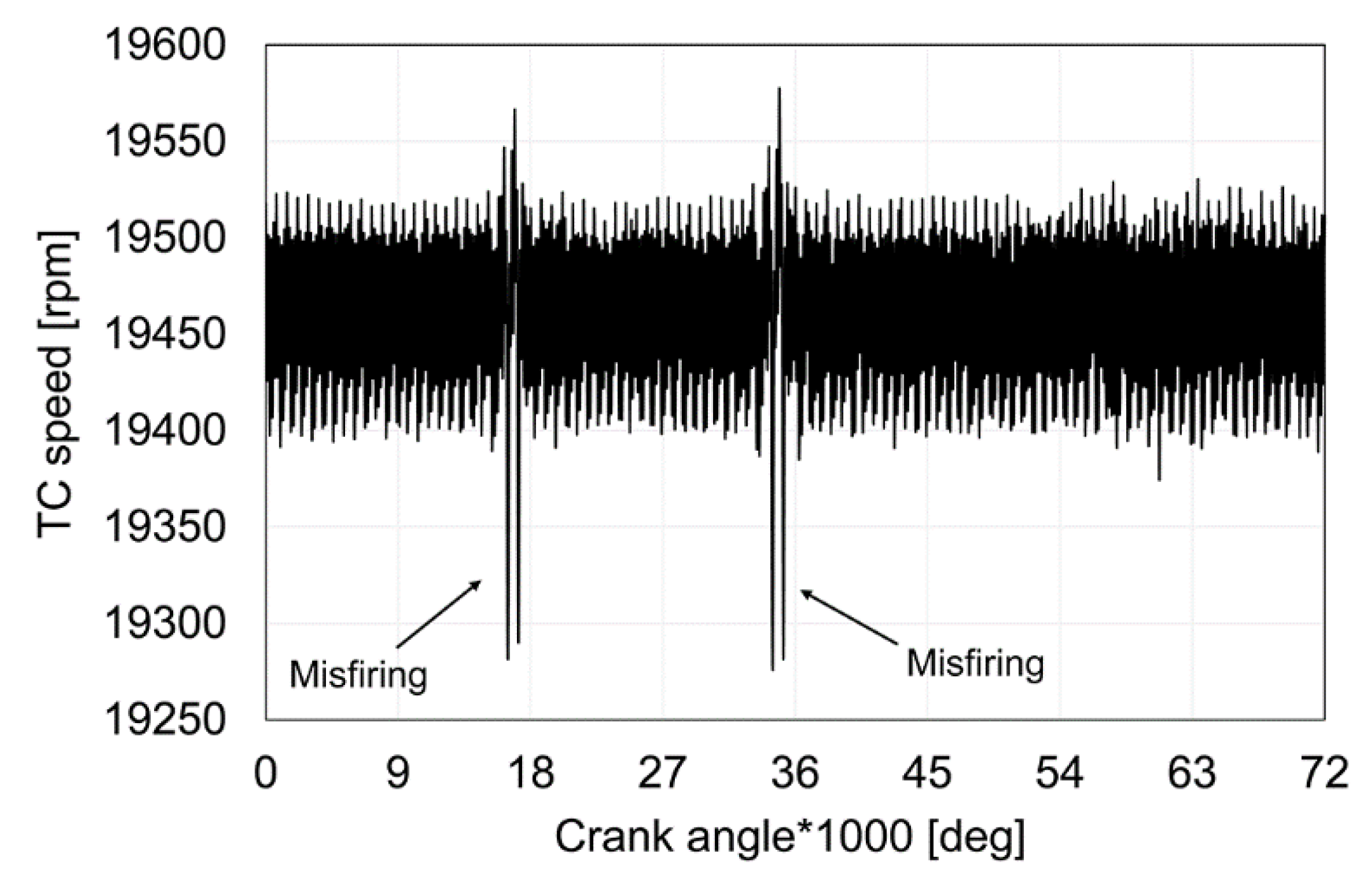
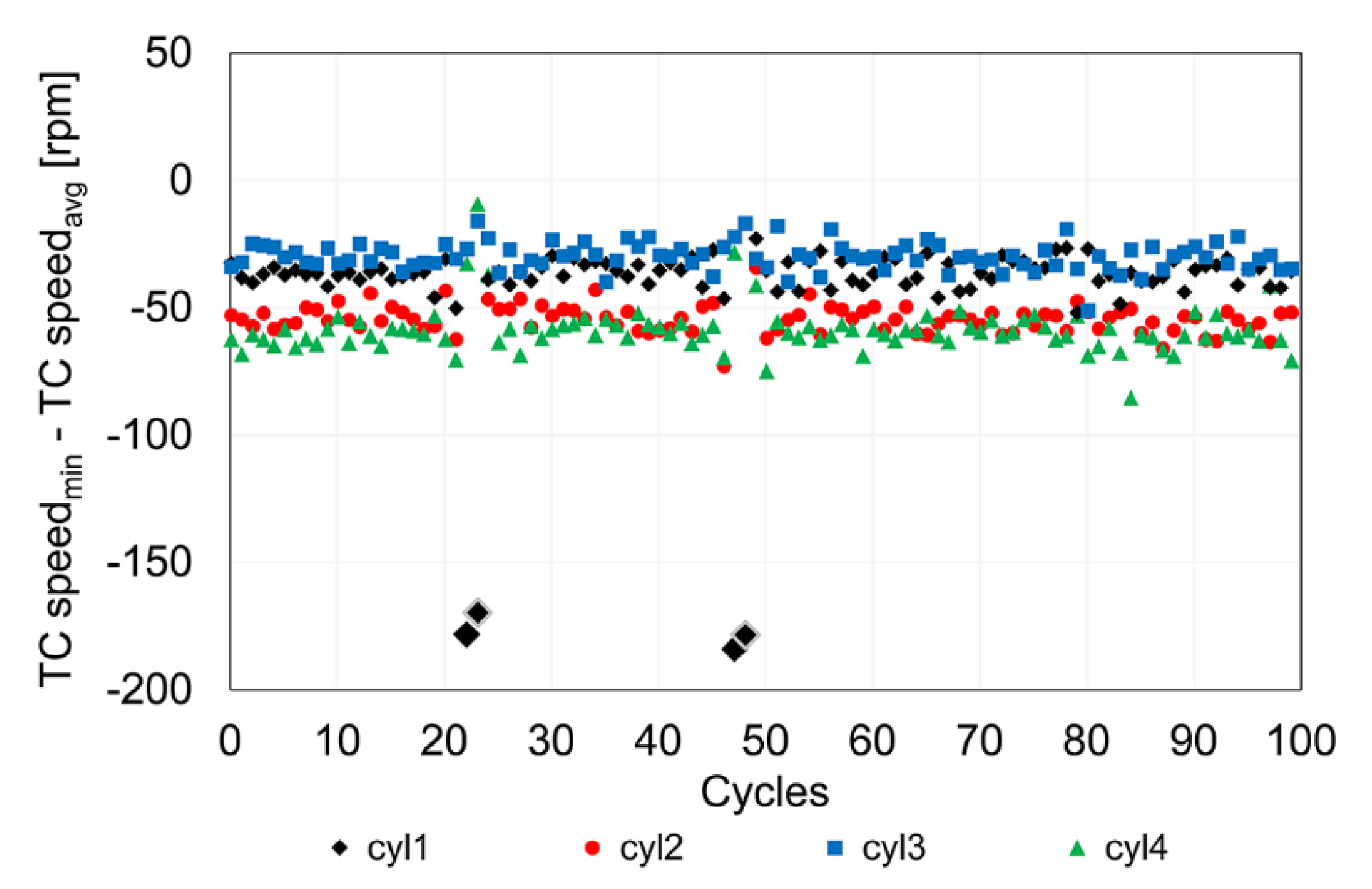
4.3. Misfiring Detection

Finally, the possibility to detect misfiring events by means of the TC speed acquisition was analyzed, since misfiring can indeed be associated and modeled as a no-injection event.
The misfiring condition was simulated at the test bench by switching off the injection in one cylinder for one, or a maximum of two, consecutive cycles. Figure 23 reports the maximum pressure in cylinders 1 and 2 for several cycles at 1000 rpm and low load with a misfiring imposed for two consecutive cycles in the cylinder 1. In order to detect the misfiring by means of the instantaneous TC speed signal (Figure 24), the best way is to define a bottom threshold on the minimum value of the velocity evaluated for each cylinder window of influence (Figure 25). By doing so, it is not only possible to detect the misfiring, but also to identify the cylinder affected by it.

5. Conclusions

In the present study, two innovative methodologies for the monitoring of the injector performance in a diesel internal combustion engine are presented and experimentally validated. The basic concept behind the procedure is the direct connection between the thermodynamic and fluid-dynamic conditions of the engine and the turbocharger. From this evidence, the two methodologies are based on the analysis of the turbocharger acceleration signal and the FFT analysis of the TC speed signal, respectively.
By combining the information derived from the FFT analysis within a neural network structure, it is possible to detect the fuel quantity injected in each cylinder. Thanks to the fourth order module of the signal, it is possible to measure the total injected fuel in the engine, while the phases and modules of the other three orders allow one to detect if there is an injection inhomogeneity, in which cylinder(s) the injected fuel variation takes place and to estimate the amount of injected fuel in each cylinder.
The TC acceleration method is based on the derivative of the instantaneous TC speed. The Turbo Charger Acceleration Factor (TCAF), defined as the maximum acceleration value reduced by the average calculated for each cylinder contribution window, is able to detect the fuel quantity injected in each cylinder.
Both the methodologies have been experimentally verified by dedicated test bench analyses carried out on a Yanmar four-cylinder compression ignition engine with direct injection for marine application (42 kW @2750 rpm). Two sets of injectors, a new one and a time-deteriorated one, were used. The experimental tests confirmed the reliability of the methodologies for the injector performance monitoring, and their ability in detecting possible variations due to system aging (e.g., when an injector is deteriorated). The FFT method, combined with a neural network structure, showed a lower error in the detection of the injected fuel and a wider application inside the working area of the engine with respect to the TCAF method that works properly only at medium–low engine speeds. However, the TCAF method is computationally lighter in the future perspective of implementation in the ECU. Moreover, considering the linear correlation that links the TCAF factor to the injected quantity in the cylinder, it requires a faster calibration phase than a neural network structure. In this view, the methodology can be easily applied to a different hardware after recalibration.
A hybrid approach for the diagnostic and correction of the injector performance in a turbo diesel engine was also conceived. The continuous monitoring of the injector performance and failure detection can be performed by means of the FFT analysis of the turbocharger speed in the whole operating range of the engine without applying the NN structure. In case of failure, the percentage correction factor of the deteriorated injector is determined by means of the TCAF method once the control unit has decreased the engine speed.
Future developments will focus on the development of an onboard control system that is able to use the information coming from the instantaneous TC speed sensor by using the methodology proposed here for the monitoring of the injection system. Furthermore, the possibility of using the TC speed sensor combined with other onboard sensors for a detection strategy of other typical faults of diesel engines will be experimentally verified.

Author Contributions

Conceptualization, M.B. and G.V.; methodology, M.B., G.V., A.B. (Alessandro Bianchini) and G.F.; software, M.B., G.V. and L.R.; validation, L.R.; formal analysis, A.B. (Alessandro Bianchini); resources, A.B. (Alessandro Bellissima), R.M., G.A. and G.F.; data curation, M.B., G.V. and A.B. (Alessandro Bianchini); writing—original draft preparation, M.B. and G.V.; writing—review and editing, A.B. (Alessandro Bianchini); visualization, A.B. (Alessandro Bianchini); supervision, R.M., G.A., A.B. (Alessandro Bellissima), A.B. (Alessandro Bianchini) and G.F.; project administration, A.B. (Alessandro Bellissima) and G.F.; funding acquisition, A.B. (Alessandro Bellissima) and G.F.

Funding

This research received no external funding.

Conflicts of Interest

The authors declare no conflict of interest.

References

  1. Luján, J.M.; Guardiola, C.; Pla, B.; Reig, A. Optimal control of a turbocharged direct injection diesel engine by direct method optimization. Int. J. Engine Res. 2018, 1468087418772231. [Google Scholar] [CrossRef]
  2. Mohammadpour, J.; Franchek, M.; Grigoriadis, K. A survey on diagnostic methods for automotive engines. Int. J. Engine Res. 2012, 13, 41–64. [Google Scholar] [CrossRef]
  3. Kyrtatos, N.P.; Tzanos, E.I.; Papadopoulos, C.I. Diesel engine control optimization for transient operation with lean/rich switches. Int. J. Engine Res. 2003, 4, 219–231. [Google Scholar] [CrossRef]
  4. Asad, U.; Zheng, M. Diesel pressure departure ratio algorithm for combustion feedback and control. Int. J. Engine Res. 2014, 15, 101–111. [Google Scholar] [CrossRef]
  5. Kamimoto, T. A review of soot sensors considered for on-board diagnostics application. Int. J. Engine Res. 2017, 18, 631–641. [Google Scholar] [CrossRef]
  6. Tschanz, F.; Amstutz, A.; Onder, C.H.; Guzzella, L. Control of diesel engines using NOx-emission feedback. Int. J. Engine Res. 2013, 14, 45–56. [Google Scholar] [CrossRef]
  7. Chiatti, G.; Chiavola, O.; Palmieri, F.; Piolo, A. Diagnostic methodology for internal combustion diesel engines via noise radiation. Energy Convers. Manag. 2015, 89, 34–42. [Google Scholar] [CrossRef]
  8. Barelli, L.; Bidini, G.; Buratti, C.; Mariani, R. Diagnosis of internal combustion engine through vibration and acoustic pressure non-intrusive measurements. Appl. Therm. Eng. 2009, 29, 1707–1713. [Google Scholar] [CrossRef]
  9. Albarbar, A.; Gu, F.; Ball, A.D.; Starr, A.G. Acoustic monitoring of engine fuel injection based on adaptive filtering techniques. Appl. Acoust. 2010, 71, 1132–1141. [Google Scholar] [CrossRef]
  10. Elamin, F.; Gu, F.; Ball, A. Diesel Engine Injector Faults Detection Using Acoustic Emissions Technique. Mod. Appl. Sci. 2010, 4, 3–13. [Google Scholar] [CrossRef]
  11. Albarbar, A.; Gu, F.; Ball, A.D. Diesel engine fuel injection monitoring using acoustic measurements and independent component analysis. Measurement 2010, 43, 1376–1386. [Google Scholar] [CrossRef]
  12. Delvecchio, S.; Bonfiglio, P.; Pompoli, F. Vibro-acoustic condition monitoring of Internal Combustion Engines: A critical review of existing techniques. Mech. Syst. Signal Process. 2018, 99, 661–683. [Google Scholar] [CrossRef]
  13. Zhao, X.; Cheng, Y.; Ji, S. Combustion parameters identification and correction in diesel engine via vibration acceleration signal. Appl. Acoust. 2017, 116, 205–215. [Google Scholar] [CrossRef]
  14. Bizon, K.; Continillo, G.; Mancaruso, E.; Vaglieco, B.M. Towards On-Line Prediction of the In-Cylinder Pressure in Diesel Engines from Engine Vibration Using Artificial Neural Networks; SAE International: Warrendale, PA, USA, 2013. [Google Scholar] [CrossRef]
  15. Chiatti, G.; Chiavola, O.; Recco, E. Combustion diagnosis via block vibration signal in common rail diesel engine. Int. J. Engine Res. 2014, 15, 654–663. [Google Scholar] [CrossRef]
  16. Johnsson, R. Cylinder pressure reconstruction based on complex radial basis function networks from vibration and speed signals. Mech. Syst. Signal Process. 2006, 20, 1923–1940. [Google Scholar] [CrossRef]
  17. Citron, S.J.; O’Higgins, J.E.; Chen, L.Y. Cylinder by Cylinder Engine Pressure and Pressure Torque Waveform Determination Utilizing Speed Fluctuations; SAE International: Warrendale, PA, USA, 1989. [Google Scholar] [CrossRef]
  18. Rizzoni, G. Diagnosis of Individual Cylinder Misfires by Signature Analysis of Crankshaft Speed Fluctuations; SAE International: Warrendale, PA, USA, 1989. [Google Scholar] [CrossRef]
  19. Moro, D.; Cavina, N.; Ponti, F. In-Cylinder Pressure Reconstruction Based on Instantaneous Engine Speed Signal. J. Eng. Gas Turbines Power 2002, 124, 220–225. [Google Scholar] [CrossRef]
  20. Lida, K.; Akishino, K.; Kido, K. IMEP Estimation from Instantaneous Crankshaft Torque Variation; SAE International: Warrendale, PA, USA, 1990. [Google Scholar] [CrossRef]
  21. Hamedovic, H.; Raichle, F.; Bohme, J.F. In-cylinder pressure reconstruction for multicylinder SI-engine by combined processing of engine speed and one cylinder pressure. In Proceedings of the IEEE International Conference on Acoustics, Speech, and Signal Processing (ICASSP ’05), Philadelphia, PA, USA, 23 March 2005; Volume 5, pp. v/677–v/680. [Google Scholar] [CrossRef]
  22. Torregrosa, A.J.; Broatch, A.; Navarro, R.; García-Tíscar, J. Acoustic characterization of automotive turbocompressors. Int. J. Engine Res. 2015, 16, 31–37. [Google Scholar] [CrossRef]
  23. Antoni, J.; Daniere, J.; Guillet, F. Effective vibration analysis of ic engines using cyclostationarity. Part I-A methodology for condition monitoring. J. Sound Vib. 2002, 257, 815–837. [Google Scholar] [CrossRef]
  24. Le Khac, B.; Jiri, T. Approach to gasoline engine faults diagnosis based on crankshaft instantaneous angular acceleration. In Proceedings of the 13th International Carpathian Control Conference (ICCC), High Tatras, Slovakia, 28–31 May 2012; pp. 35–39. [Google Scholar] [CrossRef]
  25. Bittle, J.; Zheng, J.; Xue, X.; Song, H.; Jacobs, T. Cylinder-to-cylinder variation sources in diesel low temperature combustion and the influence they have on emissions. Int. J. Engine Res. 2014, 15, 112–122. [Google Scholar] [CrossRef]
  26. Macián, V.; Galindo, J.; Luján, J.M.; Guardiola, C. Detection and Correction of injection failures in diesel engines on the basis of turbocharger instantaneous speed frequency analysis. Proc. Inst. Mech. Eng. Part D 2005, 219, 691–701. [Google Scholar] [CrossRef]
  27. Ravaglioli, V.; Cavina, N.; Cerofolini, A.; Corti, E.; Moro, D.; Ponti, F. Automotive Turbochargers Power Estimation Based on Speed Fluctuation Analysis. Energy Procedia 2015, 82, 103–110. [Google Scholar] [CrossRef]
  28. Ponti, F.; Ravaglioli, V.; De Cesare, M. Estimation Methodology for Automotive Turbochargers Speed Fluctuations Due to Pulsating Flows. J. Eng. Gas Turbines Power 2015, 137, 121507. [Google Scholar] [CrossRef]
  29. Vichi, G.; Stiaccini, I.; Bellissima, A.; Minamino, R.; Ferrari, L.; Ferrara, G. Numerical Investigation of the Relationship between Engine Performance and Turbocharger Speed of a Four Stroke Diesel Engine. SAE Int. J. Engines 2014, 8, 288–302. [Google Scholar] [CrossRef]
  30. Vichi, G.; Becciani, M.; Stiaccini, I.; Ferrara, G.; Ferrari, L.; Bellissima, A.; Asai, G. Analysis of the Turbocharger Speed to Estimate the Cylinder-to-Cylinder Injection Variation—Part 1—Time Domain Analysis. In Proceedings of the SAE/JSAE 2016 Small Engine Technology Conference & Exhibition, Charleston, SC, USA, 15–17 November 2016. [Google Scholar] [CrossRef]
  31. Vichi, G.; Becciani, M.; Stiaccini, I.; Ferrara, G.; Ferrari, L.; Bellissima, A.; Asai, G. Analysis of the Turbocharger Speed to Estimate the Cylinder-to-Cylinder Injection Variations—Part 2—Frequency Domain Analysis. In Proceedings of the SAE/JSAE 2016 Small Engine Technology Conference & Exhibition, Charleston, SC, USA, 15–17 November 2016. [Google Scholar] [CrossRef]
Figure 1. Example of the pressure in the exhaust manifold vs. turbocharger (TC) acceleration: numerical results for a four-cylinder engine (data from [29]).
Energies 12 01420 g001
Figure 2. Example of the TC acceleration in case of two engine operating conditions (numerical results): base injection and same injection variation in cylinder 1 and cylinder 3 (-5 mg). The continuous black line is the scaled instantaneous TC acceleration reduced by the mean value for each cylinder-window.
Energies 12 01420 g002
Figure 3. Representation in the complex plan of order F1 in case of injection variations in each cylinder singularly, in case of same injection variations in two cylinders consecutive in the firing order, and in case of random injection variations in two cylinders consecutive in the firing order (focus on the negative imaginary part). Engine operating conditions: 3000 rpm. Data from [31].
Energies 12 01420 g003
Figure 4. Block scheme of the algorithm for the detection and correction of injectors fault based on the FFT methodology.
Energies 12 01420 g004
Figure 5. Tested engine at the test bench.
Energies 12 01420 g005
Figure 6. Hall effect sensor installed on the compressor case.
Energies 12 01420 g006
Figure 7. Schematic representation of the operation of the Hall effect sensor mounted on the compressor.
Energies 12 01420 g007
Figure 8. The original instantaneous TC speed signal related to one engine cycle (light grey) and the post-processed one (black). Instantaneous TC speed signal by the moving average method (88 blades). The post-processed signal is referred to the average of multiple engine cycles with the application of the pass-band filter. Data correspond to 1000 rpm at full load.
Energies 12 01420 g008
Figure 9. Injected fuel quantity at three load levels by varying the engine speeds from 1000 rpm to 3000 rpm (step of 250 rpm): data is normalized with respect to the maximum injected fuel quantity.
Energies 12 01420 g009
Figure 10. Correlation between the F4 module and the total injected fuel mass flow at different engine speeds and loads, in the case of homogeneous and nonhomogeneous injection. Data is normalized with respect to the maximum injected fuel quantity.
Energies 12 01420 g010
Figure 11. Representation in the complex plan of the F1 order at 1000 rpm and two loads in case of homogeneous injection and by varying the injected fuel in each cylinder of ± 5 mm3/cycle.
Energies 12 01420 g011
Figure 12. Representation in the complex plan of the F1 order at 1500 rpm and two loads in case of homogeneous injection and by varying the injected fuel in each cylinder of ± 5 mm3/cycle.
Energies 12 01420 g012
Figure 13. Representation in the complex plan of the F1 order at 1500 rpm and full load by simultaneously varying the injected fuel in two and three cylinders.
Energies 12 01420 g013
Figure 14. Injected fuel quantity in one cylinder. Comparison between target data and NN output data.
Energies 12 01420 g014
Figure 15. Correlation between total TCAF and total injected fuel mass flow at different engine speeds and loads (homogeneous and nonhomogeneous injections are considered). Data is normalized with respect to the maximum injected fuel quantity.
Energies 12 01420 g015
Figure 16. Correlation between the TCAF and the injected fuel quantity in the cylinder at 1000 and 1500 rpm from low load to full load.
Energies 12 01420 g016
Figure 17. Gaussian distribution of errors in the evaluation of the injected fuel at medium–low speed and different engine loads: comparison between the TCAF and the FFT methodologies.
Energies 12 01420 g017
Figure 18. Representation of the F4 module as a function of the total injected fuel in case of new injectors (black diamonds) and old injectors (grey triangles) at 1500 rpm by imposing several injection variations in the cylinders at different loads. The comparison between new and old injectors at full load and 1500 rpm in case of standard injection without imposing injection variation is highlighted with the yellow diamond and the red triangle, respectively. Data is normalized with respect to the maximum injected fuel quantity.
Energies 12 01420 g018
Figure 19. Representation in the complex plane of the first order (F1). Comparison between the new set of injectors (New) and the old one (Old) at different engine operating conditions: 1000 rpm at medium load (ML), 1500 rpm at full load (FL), 2500 rpm at full load (FL), and 3000 rpm at medium load (ML).
Energies 12 01420 g019
Figure 20. Linear correlation between the TCAF and the fuel mass flow injected in each cylinder at 1500 rpm obtained with the new set of injectors and values obtained with the old set of injectors at 1500 rpm and full load. Data is normalized with respect to the maximum injected fuel quantity.
Energies 12 01420 g020
Figure 21. Results of the injection correction on the old set of injectors in terms of TCAF. Engine operating condition: 1500 rpm at full load.
Energies 12 01420 g021
Figure 22. Results of the injection correction on the old set of injectors in terms of first order in the complex plane. Comparison between the old set of injectors before the correction (bc, red markers) and the old set of injectors after the correction (ac, black markers) at different engine operating conditions: 1000 rpm at medium load (ML), 1500 rpm at full load (FL), 2500 rpm at full load (FL), and 3000 rpm at medium load (ML).
Energies 12 01420 g022
Figure 23. Maximum in-cylinder pressure for 100 consecutive cycles at 1000 rpm and low load with a misfiring imposed for two consecutive cycle in the cylinder 1. Comparison between cylinder 1 and 2.
Energies 12 01420 g023
Figure 24. Instantaneous TC speed signal for 100 consecutive cycles with a misfiring imposed for two consecutive cycle in the cylinder 1. Engine speed 1000 rpm at low load.
Energies 12 01420 g024
Figure 25. Minimum of the instantaneous TC speed subtracted of the average value calculated for each cylinder window of influence for 100 consecutive cycles at 1000 rpm and low load with a misfiring imposed for two consecutive cycle in cylinder 1. Comparison among all four cylinders.
Energies 12 01420 g025
Table 1. Imposed and calculated variation of injected fuel in one cylinder and in the case of random injection variations in two consecutive cylinders in the firing order. Data from [31].
Imposed Fuel Variation
[% Distribution of the Total Fuel Variation]
Fuel Variation Evaluated with F1
[% Distribution of the Total Fuel Variation]
Cyl 1Cyl 3Cyl 1Cyl 3
−3.00 mg
[50%]
−3.00 mg
[50%]
−2.91 mg
[48.5%]
−3.09 mg
[51.5%]
−3 mg
[37.5%]
−5 mg
[62.5%]
−2.77 mg
[34.6%]
−5.23 mg
[65.4%]
−5 mg
[62.5%]
−3 mg
[37.5%]
−5.27 mg
[65.9%]
−2.73 mg
[34.1%]
−5 mg
[83.3%]
−1 mg
[16.7%]
−5.27 mg
[87.9%]
−0.73 mg
[12.1%]
Table 2. Tested engine technical data.
Engine TypeCompression Ignition
Strokes for cycle4
Number of cylinders4
Displaced volume2100 cm3
Stroke90 mm
Bore86 mm
Compression ratio19.2:1
Number of valves per cylinder2
Firing order1-3-4-2
TurbochargerSingle-stage turbine with WG
Compressor blades number10
Engine speed range1000 rpm ÷ 3000 rpm
Turbocharger speed range~15,000 rpm ÷ ~150,000 rpm

