Bundle Extreme Learning Machine for Power Quality Analysis in Transmission Networks
by
 , , , ,
Ferhat Ucar
1,* ,
,
Jose Cordova
2,
Omer F. Alcin
3,
Besir Dandil
4,
Fikret Ata
3 and
Reza Arghandeh
5 1
Department of Electrical and Electronics Engineering, Technology Faculty, Firat University, Elazig 23119, Turkey
2
Department of Electrical and Computer Engineering, Florida State University, Tallahassee, FL 32306, USA
3
Department of Electrical and Electronics Engineering, Faculty of Engineering and Architecture, Bingol University, Bingol 12000, Turkey
4
Department of Mechatronics Engineering, Technology Faculty, Firat University, Elazig 23119, Turkey
5
Department of Computing, Mathematics and Physics, Western Norway University of Applied Sciences, 5063 Bergen, Norway
*
Author to whom correspondence should be addressed.
Energies 2019, 12(8), 1449; https://doi.org/10.3390/en12081449
Submission received: 7 March 2019
/
Revised: 11 April 2019
/
Accepted: 11 April 2019
/
Published: 16 April 2019
(This article belongs to the Special Issue Digital Solutions for Energy Management and Power Generation)
Abstract
:This paper presents a novel method for online power quality data analysis in transmission networks using a machine learning-based classifier. The proposed classifier has a bundle structure based on the enhanced version of the Extreme Learning Machine (ELM). Due to its fast response and easy-to-build architecture, the ELM is an appropriate machine learning model for power quality analysis. The sparse Bayesian ELM and weighted ELM have been embedded into the proposed bundle learning machine. The case study includes real field signals obtained from the Turkish electricity transmission system. Most actual events like voltage sag, voltage swell, interruption, and harmonics have been detected using the proposed algorithm. For validation purposes, the ELM algorithm is compared with state-of-the-art methods such as artificial neural network and least squares support vector machine.
1. Introduction
Modern industry is entwined with technology and advanced measurement devices in the production line, industrialparks, and system management units. Technological developments also cover the communication capabilities of industrial components. The Industrial Internet of Things (IIoT) is a challenging topic of smart production through Industry 4.0. According to all these challenges and improvements in both industry and human life, every player in the system moves toward being smart such as the electrical grid transforming into the smart grid. The Smart Grid (SG) context has some solutions to the problems of conventional grids such as sustainability, reliability, and energy efficiency. Governments also have development plans to complete the transformation of their cities to “smart cities” [1]. Energy and power management systems have an important place in this transformation, and power quality monitoring is one of the essential steps. A properly-managed grid operation with power quality monitoring brings sustainability. System operators drive the switching in a rational way, and grid operation can prevent large-scale blackouts and other malfunctions [2,3,4].
Recent works have shown the advantages of using big data and machine learning applications in power quality analysis [5]. There are several intelligent methods presented such as shape-based data analytics of event signals [6,7], non-parametric and partial-knowledge detection [8,9,10], and also preliminary studies including intelligent classifiers [11,12,13,14].
To detect power quality events, existing studies in the literature have mostly used transform-based methods like Wavelet Transform (WT), Fast Fourier Transform (FFT), S-Transform (ST), and so on [15,16,17]. Transform-based methods bring coefficients from a processed signal and need a second-level step to compose the last feature set. Our method in this study is less computationally expensive with its preferred feature set. There are also model-based data-driven methods in the literature, which need an amount of data during the training period [18]. We use less data to perform the classification process. In [19], the authors proposed a version of the Gabor transform method with a type 2 fuzzy kernel-based Support Vector Machine (SVM). With this method, they had to use additional math to construct the final feature set, and the dataset used was synthetic. In [20], the authors presented a basic Extreme Learning Machine (ELM) classifier with S-transform-based features. In [21], the authors used Weighted (W)-ELM for classification of power quality events with a conventional WT method. Synthetic data were used to validate the proposed system. In our study, the dataset consists of real field signals including the most commonly-confronted issues, and we built an effective feature set with respect to the importance of processing time. When considering the methods, it is very important to recognize the computational cost. Embedded technology is a superhero of today’s industrial field to uncover on-site and mobile service options. From the previous discussion, it can be observed that a strong feature set with its lesser computational cost and machine learning-based classifier bridges the gap in the power quality event classification field. In the proposed power quality-analyzing system, we present a new bundle model, including a robust feature set and ELM variations, which have improved the performance compared to conventional methods. The feature set consists of histogram, Permutation Entropy (PE), the number of Local Peaks (LP), and instant time domain features [22,23,24,25,26]. Besides, the widely-preferred Discrete Wavelet Transform (DWT) supports the feature extraction. All components in the feature set are preferred due to their low computational costs and complement each other in extracting distinctive features of raw signals. Here, the proposed feature set can be associated with online embedded systems.
The bundle classifier in this study includes enhanced versions of ELM, which is a kind of learning algorithm for the traditional Single-Layer Feedforward Neural Network (SLFN) architecture. ELM has an extremely fast operation technique [27]. There have been many types of ELM that have improved the performance values both in classification and regression applications. Different types of ELM structures have been implemented in various fields like biomedical signal processing, power quality signals, economic analyses, and many more [28,29]. In this study, we use two different ELM models. One is the Weighted ELM (W-ELM) classifier; it is one of the improved versions of the basic ELM algorithm to increase the generalization and to reduce computational costs. W-ELM has serious advantages over basic ELM such as having a simple setup in theory and functional implementation, multi-class classification ability, and also using an additional feature mapping process. The nature of adjustable weights not only makes W-ELM acceptable for a wide range of application areas, but also brings a cost-sensitive learning [30,31,32]. In many real-world applications, researchers have commonly experienced imbalanced datasets. Processing such datasets is a hard task because of the minority and majority classes and their effect on the accuracy [33]. Aiming to cope with an imbalanced data problem, W-ELM was proposed by Zong et al. [30]. The basic point of W-ELM is assigning an extra weight matrix for each training sample considering the minority and majority classes. The impact of the minority class is strengthened with an extra weighting process and vice versa for the impact of the majority class [33]. The other preferred ELM model is the Sparse Bayesian ELM (SB-ELM), which also has highlighted features on top of basic ELM. SB-ELM uses the Bayesian optimization approach in the learning process, and it includes fewer neurons in the hidden layer because of its sparsity [34].
In this study, we can list our contributions as:
- We propose a novel algorithm with a bundle structure based on enhanced versions of the extreme learning machine algorithms for power quality event classification. Unlike conventional backpropagation and other state-of-the-art learning algorithms, the proposed algorithm completely skips the iterative process, decreasing the decision phase computational cost significantly. The bundle structure allows our algorithm to select the most accurate machine learning method by analyzing different feature selection and decision-making techniques depending on the application needed. In that sense, the selection is performed according to the implementation of the training and testing time, as well as the accuracy in the classification process.
- We propose a feature selection stage for our classifier’s bundle structure by integrating a Bayesian optimization (SB-ELM) that decreases the number of hidden nodes used in the ELM decision process significantly. Additionally, we propose a feature mapping process (W-ELM) that optimizes the weight matrix of the input layer in the ELM-based algorithm.
- We validate our proposed methodology by performing online classification based on real field Phasor Measurement Unit (PMU) measurements in transmission networks in Turkey. We utilize a segmentation process for event detection, which decreases the computational cost of the classification process significantly.
To the best of the authors knowledge, this study performs a deep analysis of ELM in the Power Quality (PQ) signal processing field for the first time. We use conventional classifiers, which are Artificial Neural Network (ANN) and Least Squares-Support Vector Machine (LS–SVM), besides the basic ELM structure, to compose an effective evaluation of the proposed system.
The rest of this paper is presented as follows: Section 2 describes the real-world dataset; Section 3 summarizes feature extraction methods and presents the decision stage with the bundle ELM classifier; Section 4 gives the experimental results of the proposed system; and Section 5 encapsulates the paper with a brief conclusion.
2. Use Case
The dataset used in this study was obtained from Anatolia, selecting troubled sub-stations. In collaboration with the Turkish Energy Transmission Company (TEIAS), we collected real field data from all over the country. The dataset was obtained from the National PQ monitoring system server, which was pre-established within the scope of the National Power Quality Project. The data were collected during the year 2015. All the events in the dataset have been measured and collected with a sampling frequency of 25.6 kHz. The measurement window was three seconds long. In the circumstances of a 50-Hz grid, a period included 512 samples per event; at the end, the whole event window included 76,800 samples. Readers may refer to the detailed technical specifications of measurement devices and the monitoring system in [35]. Considering the TEIAS statistics, the most common event types were selected from the sub-stations as seen in Figure 1.
We used MATLAB to perform triggering, segmentation, and pre-processing of the data and pattern recognition system. Table 1 shows the collected data, which included PQ events of the year 2015. Due to the high resolution of the dataset, the segmentation process played a key role in decreasing the computational time cost by processing only the event windows.
The real dataset design consisted of three-phase voltage and currents, the neutral line current, and time stamp information. Thus, we should locate the abnormal phase while running the segmentation process. After the segmentation, we would have a reduced version of the data rows for the classification process. Using the raw signal as the input to the classifier is not a proper method based on its large size. In the preliminary studies, research conducted by the authors proved that the time cost of the segmented signal in feature extraction was 25-times less than any unprocessed signal (while the time cost of the segmented data was 0.0685 s, the raw data had a time cost of 1.6489 s). The proposed study ran the segmentation steps in terms of the definition in the IEEE 1159-2009 standard and used the same rms boundaries for event zones. To compute the rms values, we determined a floating window with half-cycle sampling. An original query code design was composed in the detection of the start of the events using the specified thresholds as in the related standard. Figure 2 summarizes the whole process as a flowchart.
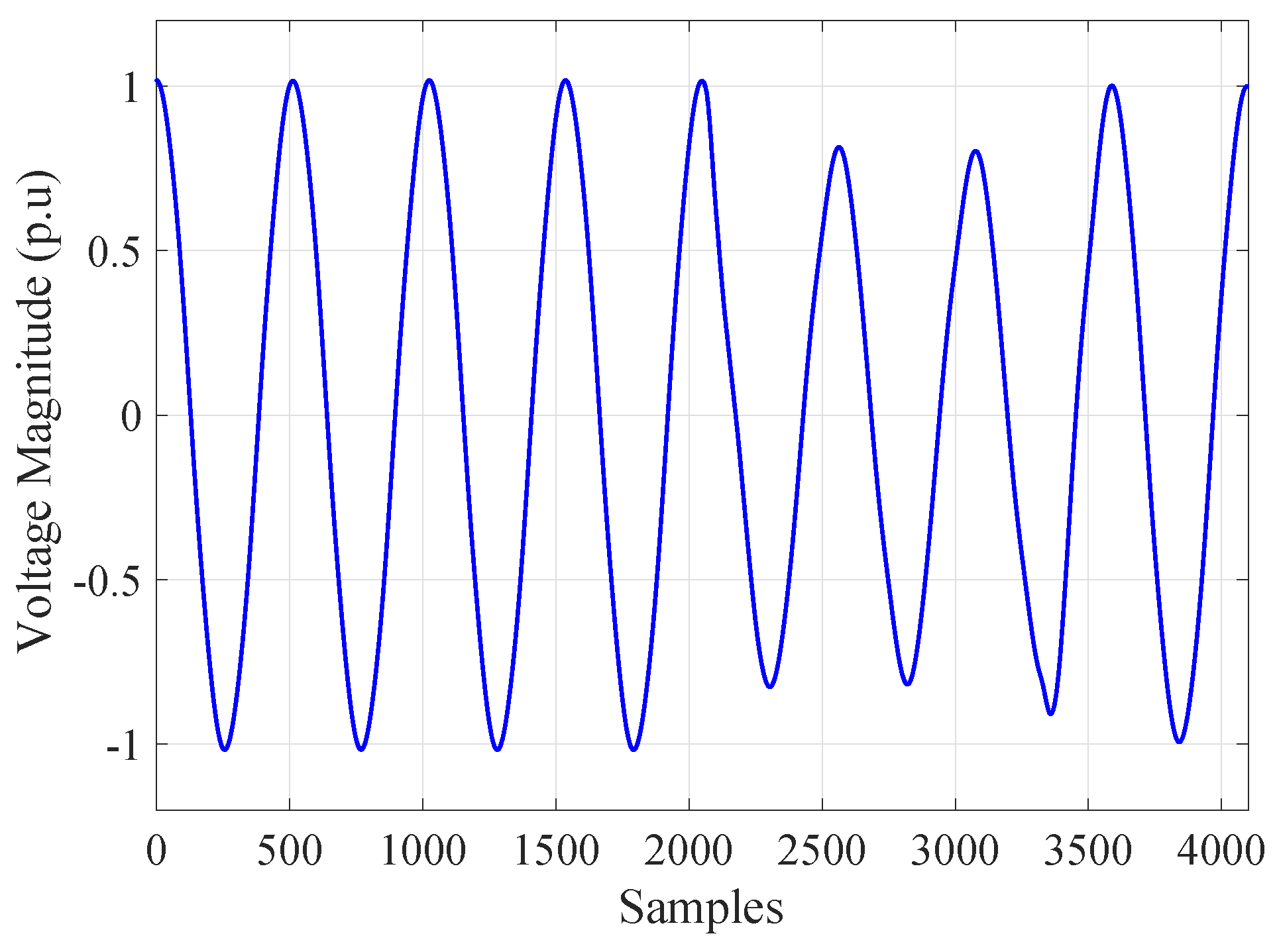
After segmentation, an event window included eight cycles also with the starting point of the disturbance. As a result, the input signal to be classified had 4097 samples (see Figure 3). As can be seen in Figure 3, we used a per-unit transformation in the magnitude value to make the normalization process better before the classification. In the voltage sag example shown, we can point out the end of the event within the specified window, but most of the events did not end within this window length.
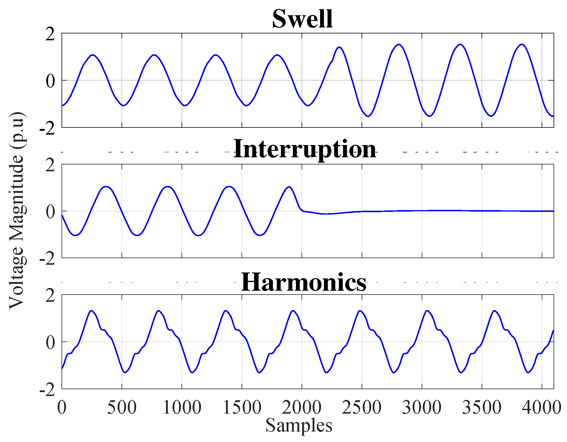
Figure 4 depicts the three samples of events in the preferred real dataset as swell, interruption, and harmonics signals.
Additionally, we picked up the normal operation grid voltage signal to compose reference signals, i.e., normal conditions. Within the dataset, the harmonics occurred rarely due to our application area of signal processing of a transmission system. For a harmonic measurement, Total Harmonic Distortion (THD) analysis was conducted giving approximately 2%–3% in all events, except harmonics. THD values for harmonics ranged between 20% and 25%. To realize an additional analysis of noisy conditions, we computed the Signal-to-Noise Ratio (SNR). The results showed that the SNR value was between the range of 47 and 55 decibels (dB).
3. Methodology
The foundation of an intelligent pattern recognition system is the dataset. The two methodological processes built on this foundation are (1) the process of the feature extracting in which meaningful and distinctive emphasis is obtained from the raw data and (2) the decision process in which these features are classified using an intelligent classifier. In this section, the methodology of the proposed power quality diagnostics and classification intelligent pattern recognition system is explained under the feature extraction stage and extreme learning machine classifier titles. The purpose of the proposed intelligent pattern recognition system here is to perform machine learning-based classification using a proper feature set of particular data, which includes real power quality events in Turkish transmission lines.
In the feature extraction process, the distinctive features generated by the traditional Discrete Wavelet Transform (DWT) and basic statistical methods, as well as histogram, instant time-domain characteristics, Permutation Entropy (PE), and local peaks that form the contribution to the literature; then, the feature set has been classified by ELM-based intelligent methods. Here, the feature extraction stage also included the Fisher vector encoding process to gather a more linear mapping of features. An effective process has been achieved with weighted ELM and sparse-Bayesian ELM structures, which eliminate the disadvantages of the basic ELM structure. All the methodology outline will be explained in detail under the following topics of feature extraction and intelligent classifier stages. The overall algorithm is shown in Figure 5.
3.1. Feature Extraction Stage
In this section, six feature extraction methods utilized in our bundle structure are described briefly. The aim is to reach a feature set that will characterize power quality event data in the best way and distinguish different classes from each other. This process, which is also called feature mapping, is defined roughly in the distribution of the selected components as the wide average distance between the classes and the narrow average distance inside the classes [2].
In addition, the features are coded by the Fisher Vector (FV) method. This transformation aims to achieve a more uniform distribution to increase the performance of the classifier structure. Although the preferred FV coding method is generally used in image processing applications, it increases the size according to the parameter values, and it has a positive effect on the classifier performance due to achieving a more uniform distribution.
3.1.1. Permutation Entropy
Permutation Entropy (PE) calculation, which is commonly used in biomedical signal processing applications, shows the complexity of the time series signal according to the neighborhood values of the samples [23,36]. The feature set obtained by the PE method was proposed firstly with this study in the power quality signal processing field. As an initial step in the calculation of the PE method, a given time series signal is converted to a symbolic sequence. Thus, the relationship is acquired between the existing values, and the previous values are based on a constant equal distance. The expression of the embedded procedure of the transformation method is shown by (1) as follows:
where m is for the embedded size parameter and l is for the time lag parameter. By a given m value, we may have possible permutations up to long. Thus, the relative frequency value can be shown by (2) in the following way:
where represents the value of the symbolized frequency in . The PE value can be calculated using (3) as follows:
Given the normalization factor , the normalized PE formula is expressed lastly in (4):
Choosing the parameter m is crucial in PE calculation [24]. If m is too small, the process may not work properly. Furthermore, a very large value of m may cause memory restrictions and malfunctions when capturing the dynamic changes in the signal [23,24]. The work in [36] recommended this value to be within the interval of . In this study, we chose the embedding parameter and time lag .
3.1.2. Local Peaks
The Local Peaks (LP) feature set consists of determining the number of local maximums for the time series signal. The detection of local peak points, which is another proposed method for power quality events, is preferred because the event signals are non-stationary and have fast amplitude variation. A local peak can be defined as a point that is larger than the neighboring values [26]. To perform peak detection, MATLAB offers the command function findpeaks, which scans through the signal samples, finding the local maxima point. For more detailed information, please see [26]. Detecting peaks in the data array is an important step for many signal processing applications. In biomedical signal processing applications, receiving local peak information from signals that indicate heart rhythm or that are related to brain function may have a vital role in the functioning of the system. In the same way, peak points’ detection can also bring important information to light for traffic intensity detection applications and signal processing applications related to solar and wind energy fluctuations. There are a number of studies that have been proposed in a wide range from conversion-based methods to peak detection to filter-centered or intelligent system-based applications [37].
Based on all the discussion above, the number of local peaks belonging to each of the event data was determined. A single feature was obtained for each signal in the dataset. The obtained sub-set of LP features was created with these values.
3.1.3. Histogram
One of the subsets that makes up the feature vector used in this paper is the subset of “histogram attributes”, which contains the histogram values of raw event signals. It is a group of operations that is used to show the cluster of columns in which the data distribution is formed according to certain criteria. Since power quality event data also refer to a numerical distribution, the number of samples in certain step values of this data distribution is obtained by the histogram process, and it is used to obtain the attributes of these numbers, which are highly discriminative. This method, which is analyzed for the first time for use in power quality event data with this study, has formed highly distinguishable attributes between the analyzed event signals.
The steps of grouping the samples within the data were done according to the voltage amplitude values, which was in the range of as the unit value conversion was performed. In the current study, the selection of histogram grouping steps/bars was made according to Sturge’s rule, given in detail in [38]. Hence, according to the calculation, the histogram attribute number was 13 per event. Prior to this article, preliminary experiments with synthetic data related to histogram attributes were published in [39].
3.1.4. Instantaneous Time Domain Methods
For a more effective classification of power quality event data with a machine learning-based decision process, the attribute set must have a rich discriminant capability. For this purpose, various instant time domain parameters have been added to the set of features, which was created step-by-step. The preferred features were derived from a number of parameters used in the field of digital modulation, especially in the field of communication [25].
Instant Time Domain (ITD) attributes were determined based on the instantaneous amplitude, phase, and frequency changes of the signal. Similar to the variable characteristics of power quality disturbance signals, processing the modulating signals such as carrier frequency, phase, and amplitude, the ITD parameters provided significant discrimination over power quality disturbance signals. The first two of the preferred attributes for this purpose were Hilbert Transform (HT)-based parameters. The HT method, based on the generation of a complex set of data from a time series signal, is a method using instant frequency determination, commonly used in the analysis of non-linear and non-stationary signals [25].
- The second attribute obtained from the ITD data () was the spectrum symmetry parameter given by a P ratio, and the mathematical equation is indicated by (6) [25]:The terms and are defined as follows in (7):where “fcn” refers to the sampling frequency () normalized with an parameter according to the number of samples (), and the mathematical expression is represented by (8). In this study, the empirically-obtained value was defined as . expresses the Fast Fourier Transform (FFT) output of the signal [25]:
- The last component () of the time domain attribute set was obtained by calculating the maximum value of the Power Spectrum Density (PSD) of the normalized and centered instantaneous amplitude expression. In particular, the PSD used in the detailed examination of non-stationary signals may contain significant distinctive highlights of the processed signal. For PSD calculation, Discrete Fourier Transform (DFT) was applied to the signal. The mathematical equation of this definition is given by (9) [25]:where represents the change of the amplitude values of the signals, which is an important feature in performing the distinction between classes. The change in amplitude between the disturbance events is a strong determinant of the differentiation of classes.
3.1.5. Basic Statistical Features
The process of extracting distinctive features from power quality event signals was continued by giving definitions of the attribute set based on the basic statistical data presented under this subsection. Without relying on any conversion method, the statistical value definitions were applied to the raw event data to create a subset with a total of 9 attributes.
Among the basic statistical definitions such as the minimum value, the maximum value, the mean, standard deviation, and median values of the data series, as well as the root mean square (rms) value, the mode value of the data array, skewness, and kurtosis parameters were also obtained. The rms value used in this subset was the statistical rms value defined independently of the electrical point of view. In the formulation to be calculated for any X event, the result of (10) consisted of a single value because the calculation window contained the entire data length (n samples).
3.1.6. Discrete Wavelet Transform
The DWT, based on the use of filter banks, was proposed in 1988 by the French mathematician Stephane Mallat. With this process, the signal is divided into detail and approximate components [2]. The most distinctive difference of the DWT, which is similar to the continuous wavelets, is that the scale “a” and shifting “b” components have a discrete spaced structure. The most important element here is that the selected wavelet functions must be within their own structure and within the extension of the orthogonal transformation. The basic expression of the DWT method is defined by (11):
where n shows the shift in time and m shows the expansion.
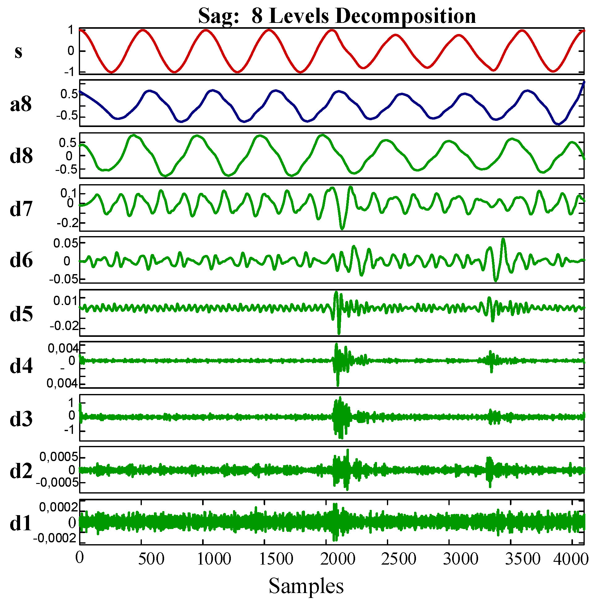
In this study, the Multi-Resolution Analysis (MRA) form of the DWT process (DWT-MRA) was designed as an 8-level decomposition by using the “daubechies4” wavelet function. These parameters were determined as a result of the literature research [40].
3.1.7. Fisher Vector Encoding
In this paper, the Fisher Vector (FV) coding method was used to classify the feature set more effectively at the decision stage. By mapping the features with the FV kernel function structure, a high-dimensional distribution was obtained with a larger number of elements. The FV coding structure is generally used as an alternative to the visual mapping method of Bag of Words (BoW) in image processing applications that contain a large number of attributes. The FV coding method is also defined as an improved version of the BoW mapping method [41]. In the literature, it has been observed that it supports successful classification results in time series signal analysis applications as well [29,41]. For this reason, it is suggested in the study that the method be adapted to the set of characteristics obtained from the power quality disturbance events as a contribution to the literature.
The basis of the FV coding method is the Gaussian Mixture Model (GMM) adaptation, which is a parametric model for the attribute set. In FV coding, the log-likelihood derivative is calculated using the parameters of the GMM model. Thus, a representation of the average of the first and second-degree difference values between the element distribution and each element of the centers in the GMM distribution is revealed. As its most basic and brief explanation, the FV coding is to perform the clustering of the differences with certain parameters [41,42].
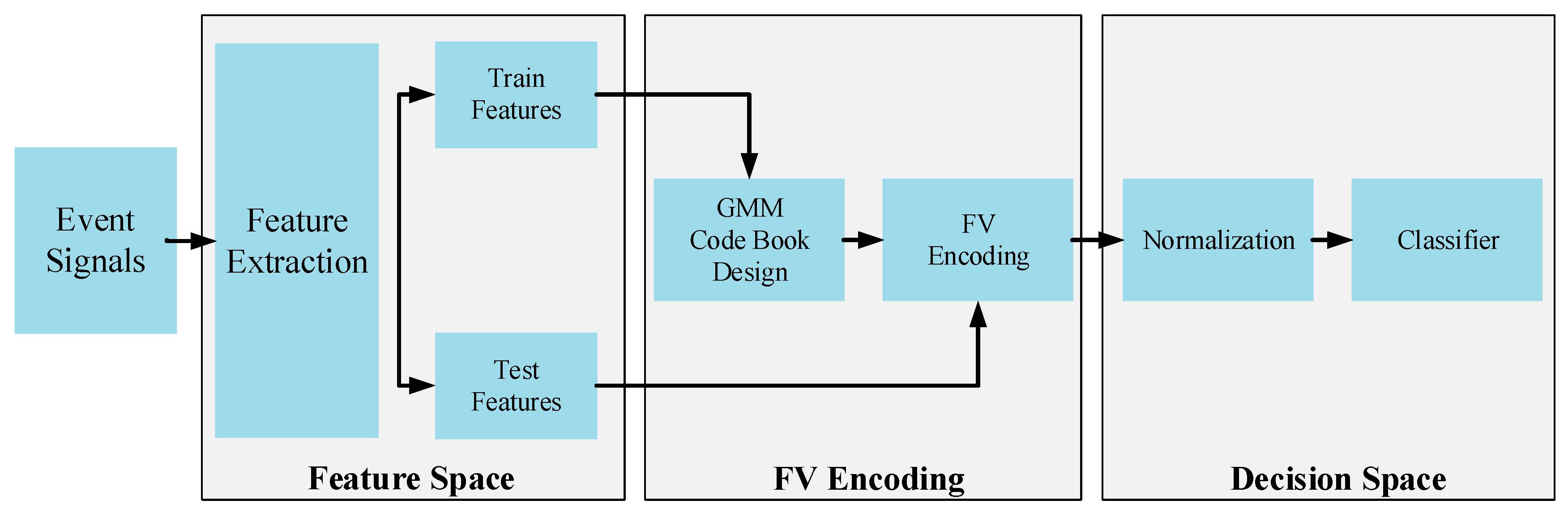
Figure 6 shows the general block diagram of the above explanation. When the steps in the block diagram were analyzed, we see that the features obtained from the dataset were divided into training and testing. GMM parameters were obtained using only training data, and a codebook was created. As a result of this process, the feature set was obtained. While obtaining the feature set to build the test data, GMM parameter values obtained from the training data distribution were used. This was not calculated again for the test data. Thus, the and feature vectors were given as input to the classifier after FV encoding. In this study, because of the parameter selection of the FV method, FV encoded feature set doubled in size, i.e., the FV encoded feature set had twice the number of elements.
3.2. Extreme Learning Machine Classifier
ELM, as recommended by Huang et al., was the learning algorithm used for the Single Hidden Layer Feed-Forward Neural Network (SLFN) [27]. In contrast to gradient-based feed-forward nets, in the ELM method, input weights and bias values are generated randomly, while analytical methods are used to calculate the output weights. With this method, the learning process becomes extremely fast. In addition to its fast learning ability, ELM has better generalization performance compared to feed-forward networks with the traditional back-propagation learning algorithm [28]. In ELM method, input and hidden layer connections are fixed. The links that connect the hidden layer to the output are adjustable [43].
In this respect, the basic mathematical properties of the ELM method, which can be accessed with all the mathematical details with [27], will be discussed, briefly. Before the definition of the improved variations used in this article, the explanations will be started by touching on the most basic ELM structure.
For N samples to be used in the training process, consider a training dataset in the form of . Here, the input vector is , and the output values are in d-dimensions. The output function of an ELM structure with L neurons in the hidden layer can be expressed as (12) [34]:
where is the component that performs the hidden layer feature mapping based on the input vector and the output weight vector. Bias values were added to each inner product. The hidden layer activation function is . Equation (12) is more simply indicated by (13):
where is the feature mapping matrix with dimension and can be presented in detail as:
Here, the ith row of the matrix defines the output vector of the hidden layer for a sample x. Calling back to Equation (13), it has a linear system solved as:
where states the Moore–Penrose inverse [44] of . Here, C is used as the regularization parameter for ELM, being more effective in multi-class classification [28].
Equation (15) expresses the simple form to be solved when defining output values [27]. In traditional algorithms, iteration steps are needed to get desired outputs, but ELM tries a one-time solution to deal with the same situation without any iterative actions. As an additional explanation in the optimization perspective, the ELM process tries to obtain and minimizations. Therefore, we can describe the solution of (13) as [33]:
where the vector is for the training error of the m output nodes for each training sample . We can reach the same solution as in (15) via the Karush–Kuhn–Tucker (KKT) theorem [33].
ELM also responds to the multi-class classification process. Assuming N training sample inputs and outputs for m number of classes, we can state a vector with a length of m for each sample as:
Here, the ELM output function can be derived for a given sample as [27,33]:
where is the vector of the output function. Readers may choose (19) for the test progress of the classifier according to the prediction label of [33].
3.2.1. Sparse Bayesian Extreme Learning Machine
The basic ELM method is influenced by the following two adverse events: (1) The ELM structure solves the equation, which calculates the output weights, by using the Moore-Penrose generalized matrix inverse. This point can easily be influenced by the problem of over fitting since it is some kind of least squares minimization learning method. This can be worse if the training set does not fully represent the characteristics of the data to be processed. (2) The classification accuracy of the ELM is severely affected by the number of hidden layer neurons. An ELM model designed for practical applications can often have a number of hundreds or thousands of hidden layer neurons [34]. The first issue that will be affected by this situation is, of course, the embedded systems that the real applications work on and the memory values they have. In a low-cost application, a high-cost memory structure is not required to run the large-scale ELM model. Therefore, the solution steps to be achieved by reducing the size of the model without compromising the performance of the model output are required [2,34].
In order to eliminate the initial negativity above, although methods such as the kernel ELM with L2-type arrangement have been proposed, it is very difficult to use them in applications containing large data due to their computational costs and workloads [34].
The present methods, which aim to find the most proper number of neurons by running an optimization in the ELM hidden layer, utilize an incremental learning method, and many of them fit only regression applications. Bayes ELM (BELM), which is based on the Bayesian approach, has avoided over-fitting by estimating the probabilistic distribution of output values by providing an advantage in machine learning methods to calculate output weights with high generalization performance. This situation has not been able to provide a complete solution since it contains complex calculations and cannot be adapted to the classification process. In this article, the Sparse Bayesian ELM (SB-ELM), which is based on the sparse Bayesian learning approach proposed in [34], was adapted for power quality event classification.
The SB-ELM structure is a method that finds the sparse representations of the output weights and reaches the solution without adding or deleting the number of hidden layer neurons after the coincidentally-produced hidden layer parameters as in the conventional ELM structure. It was aimed at finding sparse estimates of the () values determined as output weights. In the SB-ELM, the sparse process is based on the Automatic Relevance Determination (ARD) method used in the Bayesian statistical approach. Here, some values were set to zero by scanning the Hyper-Prior (HP) distribution over the output weights . According to the degree of relevance in the distribution of hyper-prior , most of the output weights were sparse, and the hidden layer neurons were pruned and simplified. All these process steps show that the SB-ELM collects positive aspects such as high generalization and sparsity as in the SB learning approach and universal approximation and effective learning speed as in the basic ELM structure.
3.2.2. Weighted Extreme Learning Machine
W-ELM is an ELM development that is proposed as a solution to the problem, called unbalanced learning. However, it is also used in the balanced learning context. In W-ELM, the valued feature according to the basic ELM is to apply an additional weighting process to the classes in the learning phase, i.e., an additional weight assignment is made to each training instance. Theoretically, an -sized diagonal matrix is assigned to each training sample (). The weighting process makes the effect of the minority class more strengthened by defining a larger weight value, and vice versa for the majority class. This approach is superior to the traditional architecture of the W-ELM structure, as well as reducing the computational cost with adaptive weight characteristics. Although W-ELM can be more easily adapted to multiple classification applications than the basic ELM structure, it provides a more regular and convenient feature mapping. Here, we present a brief discussion of W-ELM. For a detailed presentation of W-ELM, please refer to [30,33].
It was stated that the purpose of the basic ELM method was to minimize the components of (20):
If the specified additional weighting matrix is added to the expression by which this solution is handled from the perspective of optimization, the expression given with (21) is obtained:
where the vector is the error value of the m output nodes for each training data instance. The expression creates the feature mapping in the hidden layer based on the parameters. The solution of (21) is expressed by (22) for a model with N training samples and L neurons in the hidden layer using the KKT theorem [33]:
For detailed information about how to determine the weights for minority and majority classes, please refer to [30].
4. Results and Discussion
In this section, experimental results of proposed models are presented. First, the evaluation process is explained briefly, then some findings of the feature extraction stage are presented. Finally, the findings from ELM, SB-ELM, and W-ELM are given. In the evaluation process, specific to this article, an additional test procedure was considered for the k-fold cross-validation method.
The main dataset consists of 1500 samples obtained at the end of the feature extraction process; the training set (1000 samples) and the test set (500 samples). Both sets consisted of five event classes with an equal number of distributions. In the model determination method used in this study, the training process of the proposed machine learning algorithms was performed with the 10-fold cross-validation method. In other words, the training process, including a validation process in itself, as described above, is the 10-fold cross-validation method’s result, and those models have ten performance values.
Among the 10 models, the model with the highest accuracy value was chosen, i.e., the “selected model” was determined. Experimental results were gathered by applying the test dataset, which was not used during the 10-fold cross-validation. Thus, all proposed algorithms were subjected to the training and testing process by creating the most difficult conditions. In addition, a model proposal and application of an integrated solution to the problem of the end-user were also determined. As a result of the study, a model was saved for each individual scenario in which each algorithm was evaluated, and a power quality event classifier product package had been obtained in such a way as to appeal to the end user since these models were of a structure that can be used in embedded devices. All analyses during this study were performed with original code files and directories written in MATLAB environment. This includes the preparation of the dataset and the pre-processing. The workstation on which the codes were run consisted of a hardware architecture with a 32-GB memory (RAM) and a dual processor consisting of eight cores with a basic frequency of 2.1 GHz.
The evaluation criteria used for the proposed model were determined based on the creation of a table called the confusion matrix and selected from the most preferred criteria in the literature as follows: accuracy, sensitivity, and specificity [45,46].
In this article, the normalization method preferred was the zero average and unit variance method and commonly referred to as the z-score. The mathematical expression of this method is given by (23).
In the z-score () calculation here, the average value of the dataset consisting of elements is represented by , and s is the standard deviation of the data distribution.
4.1. Findings from Feature Extraction Methods
In the following, the findings of the FE methods are presented graphically, and also, tables of the attribute lists are given.
In the PE method, there were seven attributes, as listed in Table 2. Besides the normalized PE value as a feature, we took into account the histogram of the PE distribution. The number of the PE features was six due to the selected value of . It had a permutation number of six, and the histogram counted those six bins as additional features. Briefly, a single PE value and six histogram values were collected as the PE feature set.
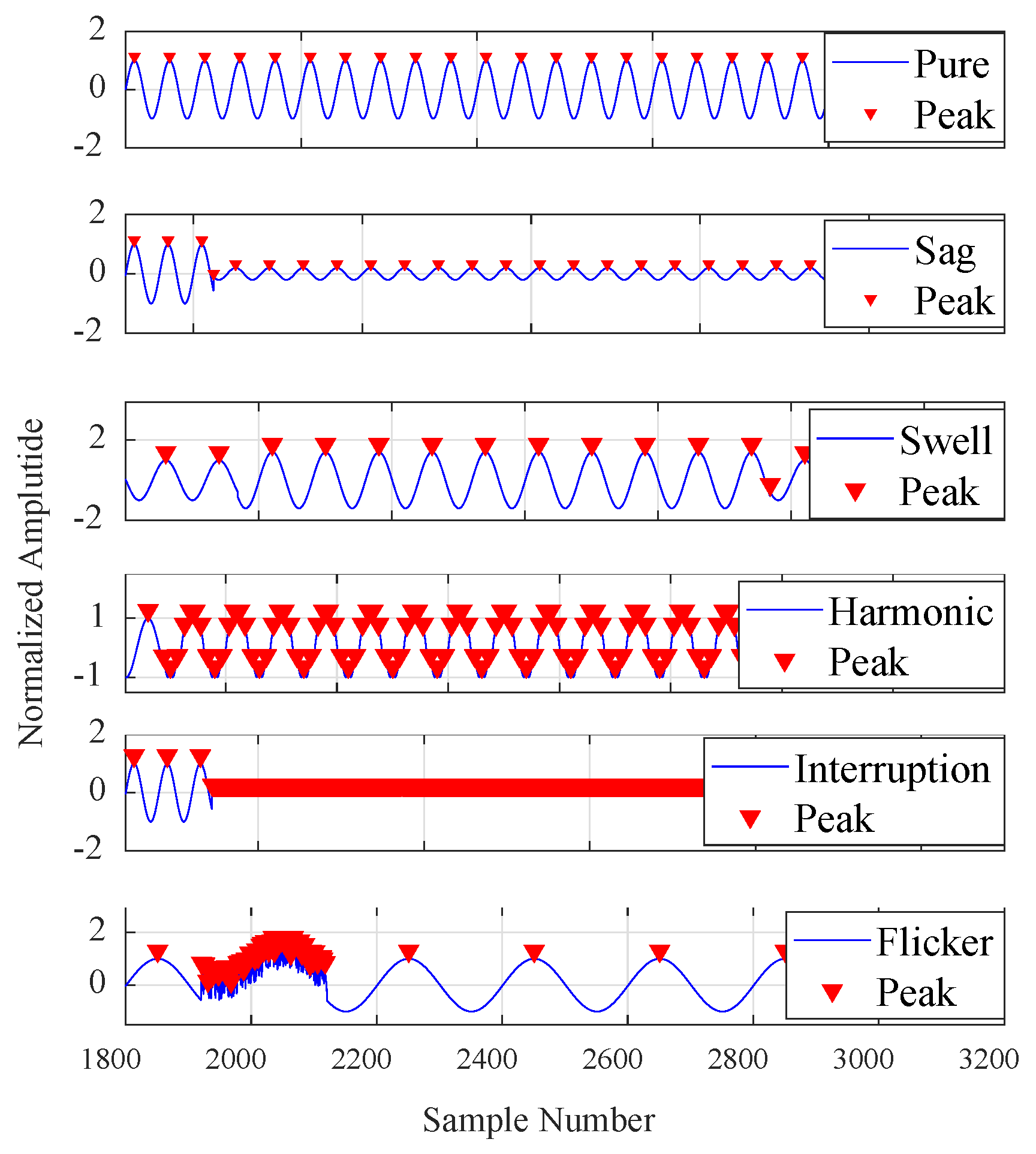
In Figure 7, one can see the local peaks for some selected event samples. Here, we used only a single attribute value of LP for each event signal.
Figure 8 shows the findings of the histogram method graphically for some selected events.
Figure 9 shows the detail and approximate vectors obtained from the DWT-MRA of a sample event signal. In the figure, represents the detail vectors, is the approximate vector, and s represents the original signal.
As listed in Table 3, we applied some more math to the DWT-MRA coefficients. To reduce the length of the detail vectors, the following operations were used: standard deviation, Shannon entropy, the mean value of the signal energy data, and the energy of the approximate coefficient [39,47].
The main feature set, the so-called Full feature Set (FS), used in experiments consisted of 51 elements. The FV encoded Full feature Set (FV-FS) included 102 elements. The sets of features derived from the methods detailed in Section 3.1 are summarized in Table 4.
4.2. Findings from ELM
The number of parameters that need to be determined is very low in the design process of a classifier using the ELM method. This can be defined as an advantage of the method used in the model. The design parameters of the ELM classifier are given in Table 5.
Figure 10 demonstrates the performance of an ELM structure using the unipolar step activation function defined as hardlim in the MATLAB code design, corresponding to the number of hidden layer neurons. It was observed that the ELM classifier structure with the 375 neuron determined as the parameter produced the highest performance value, i.e., the mean accuracy value. Each experiment, in order to determine the parameters, was repeated 100 times, and the performance evaluations were sorted by the average accuracy data. In addition, in each experiment, training and testing procedures were performed with a 10-fold cross-validation scheme. The differentiable functions such as tangent sigmoid (tansig), radial basis (radbas), and sigmoid (sig) functions, which can be used in our algorithms, were examined experimentally, and the best average accuracy value was observed with hardlim usage.
Table 6 shows ELM’s overall performance details. In the Accuracy columns, 10-fold cross-validated training accuracy and the standard deviation (±) and variance (var) values are given. In the last two columns, Sensitivity (Sens.) and Specificity (Spec.) criteria are given, respectively.
When Table 6 is examined in detail, it is seen that the highest performance value in terms of test accuracy belonged to FS with 51 elements. Training and test times were both acceptable. Considering the set of training samples, especially the 1000 data, the average value of the training times was 0.9516 s for the FS, indicating that the ELM method can produce highly-effective results in terms of computational speed.
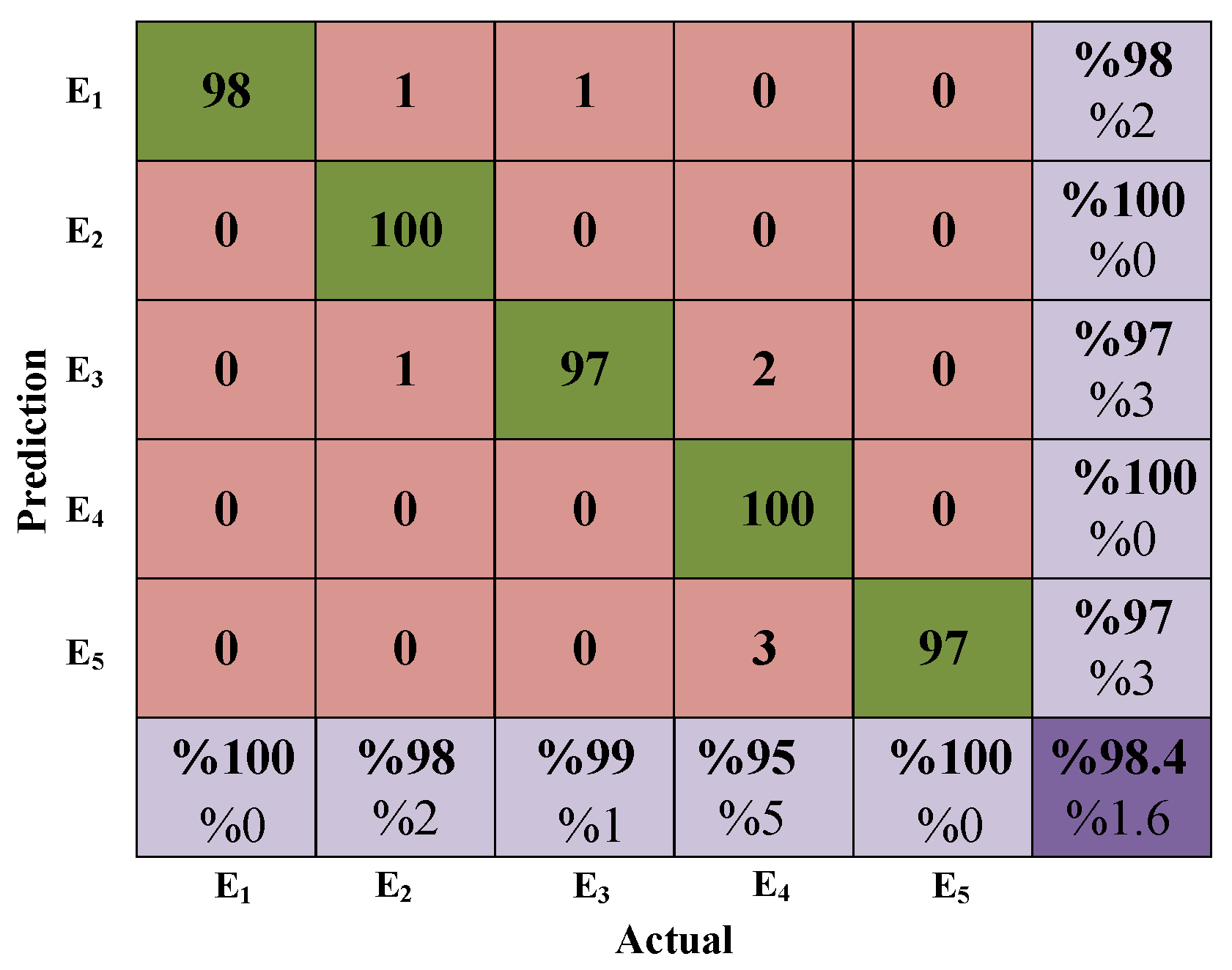
In order to examine the general results of the ELM method in more detail, a table of performance values according to the classes, which indicate the correct classification number of the classes in the test data, was also formed. Here, because the test data contained 100 samples per class, the number of correctly-categorized samples can be read as a percentage by this value. The results obtained in this direction are presented in Table 7. From this point, it is seen that FS attributes correctly predicted all samples in both the sag and interruption classes.
The Confusion Matrix (CM) given in Figure 11 was obtained with the FS, which produced the highest performance value among the ELM method’s general results. Here, the rows of the CM represent the sample numbers of the predicted classes, while the columns represent the sample values of the actual classes. Each row/column accuracy ratio is also summarized as the percentage value in the lower and most right cells in the matrix. Below this ratio, percentage error values are also included. It is important to note that the accuracy rate of each column gives us the sensitivity value of the classes; the accuracy rate for each row indicates the independent accuracy values of each class.
4.3. Findings from SB-ELM
The sigmoid function was used as a hidden layer activation function in the experiments of the SB-ELM classifier structure and is expressed as . Here, and b refer to the weight (synapse) randomly determined at the beginning of the operation and bias values added to each weight. These values are in a uniform distribution with a range. In practice, these random parameters can have an effect on performance. Therefore, in the SB-ELM algorithm, an improvement on these values was carried out in each cycle processed during the cross-validation, and a seed tracking interval was defined so that each cross-validation cycle was repeatedly run in this range. If the hidden neuron number L and the seed tracking value s that generates randomized weight and bias values are defined as , SB-ELM was performed with the intervals of with a hidden layer neuron number increase of 20 in every loop. Details on the SB-ELM parameters are summarized in Table 8.
In the SB-ELM experiments, it was obvious that the training periods would be much longer than the basic ELM method since the scanning algorithms were iterative (each experiment was 250 cycles). Given that the model to be obtained as a result of the optimizations would gain the ability to produce better generalization and accuracy than the basic ELM structure, this one-time delay in the model determination phase is feasible. Table 9 shows the overall performance values of the SB-ELM method.
When the Table 9 is examined in detail, it is seen that the highest performance value in terms of test accuracy was for FS with 51 elements. When the duration of training for all scenarios is examined, it is observed that there was a significant increase compared to the basic ELM structure. One point that needs to be emphasized here is that the standard deviation and variance values of the training accuracy in the SB-ELM structure were very small. This situation shows us that the SB-ELM structure is more stable and robust.
Findings showing that SB-ELM method had a simpler model are presented in Table 10 where the numbers of active neurons are given. As can be seen here, the number of hidden layer neurons, which was set at 375 in the basic ELM method, was reduced to a very small number in the SB-ELM method and was set to five and six. Therefore, the test times obtained in the SB-ELM method were very low.
The results given in Table 11 show the test accuracy of the SB-ELM method on the basis of classes. As can be seen in detail, the results obtained with almost half of the 28 experiments performed can be interpreted as having a very good classification rate. Specifically, there was a large number of datasets reaching the value of 100% in the sag and interruption events.
The CM shown in Figure 12 was obtained with FS. When the given CM was examined, almost all of the samples of all classes were classified correctly. As can be seen, only a single interruption event was confused with a harmonic. As a result, it is clear that only s even misclassifications occurred.
4.4. Findings from W-ELM
Unlike the basic ELM method, the parameters determined for W-ELM, which is solved with an additional weight matrix according to the density of the classes, are listed in Table 12.
W-ELM parameters given by Table 12 were empirically obtained by the application of a repetitive series of experiments. For the empirically-defined regularization parameter (C), the values in [30] were also referenced in the range. Among the different activation functions, the unipolar step function, as in the ELM structure, produced the best accuracy value. In the analysis of the performance values corresponding to the number of hidden layer neurons, it was found that the highest accuracy value was achieved in the 2500 neuron value. The graphical representation of this situation is given in Figure 13.
When Table 13 is examined in detail, it is seen that the Fisher vector encoded full set (FV-FS) gave the highest performance value in terms of test accuracy. This feature set, which was derived from all feature extraction methods whose theoretical substructures were given, also showed high-performance values at the point of sensitivity and specificity criteria. The sensitivity value generated by this set appeared to be one, which is an indication that the model was accurately predicted with almost all inter-class samples. In the findings of the W-ELM method, it was seen that there was a slight increase in the duration of training for all scenarios compared to the basic ELM method. The reason for this is the additional weighting process used to increase the generalization ability and the need for more hidden layer neurons to achieve the result. In this method, the standard deviation and variance values for the training results showed that the distribution of the accuracy sequence obtained from 10-fold cross-validation was regular, and performance values showed a distribution close to the average value.
The CM given in Figure 14 was obtained with the FV-FS set, which showed the highest performance value in the W-ELM method overall result list. When this CM was examined, it was seen that all of the sags, swells, and interruptions were correctly classified. Two of the normal conditions events were misclassified with sag event. Similarly, the single harmonic class was confused with the swell event, and the incorrect classification was performed. As a result, only three inaccurate classifications were performed. As can be seen from the overall accuracy value, almost all test sets were classified correctly.
Table 14 shows the test accuracy of the W-ELM method based on classes. As can be seen from this table, the FV-FS, which produced the highest test accuracy value, had a highly accurate estimation capacity between classes and correctly predicted all sags, swells, and interruptions in the test dataset.
4.5. Model Performance Comparison
The highest performance values obtained from all of the analyses performed during the study are summarized and listed in Table 15. Among the table rows, the best performance value and the scenario are highlighted.
When Table 15 is examined, it was the W-ELM algorithm that provided the best performance in the power quality event classification process with FV-FS in the test dataset. Although the performance values of each of the three models proposed here were very close to each other, this is an advantage of this method that the sensitivity value of the W-ELM was higher. The SB-ELM algorithm produced nearly the same test accuracy as the W-ELM algorithm. However, the basic ELM structure also had the lowest training and testing times. Considering all the results, the W-ELM method that produced the best performance values came to the fore as the proposed model using the FV coded Full Set (FV-FS).
The proposed model was compared with the main two methods that have been used for a long time in the literature, Artificial Neural Networks (ANN) and Least Squares Support Vector Machine (LSSVM). Since the ELM method is the learning algorithm used for a single-layer feedforward network architecture, the ANN structure is designed to contain a single hidden layer. The hidden layer neuron number was 20, and the activation function was set to tangent sigmoid. The linear activation function was used in the output layer. These values were determined empirically as a result of a series of parameter determination experiments. In the code design used for the LSSVM method, the parameters were determined in the experiment by self-adaptation. The theoretical infrastructure of this methodology and the more detailed information can be consulted from the study [48]. The code design used here was also performed with the MATLAB toolbox published by the authors of [48].
Figure 15 presents the comparison of the LSSVM and ANN performance of the proposed W-ELM model with the box plot image. The benchmark was the average accuracy because each classifier was evaluated using 10-fold cross-validation with 1000 sample training data to obtain accuracy distributions for the methods. As can be seen from the graph, the average accuracies of the W-ELM and LSSVM methods were very close to each other. However, the resultant distribution was more uniform in the W-ELM method. In Figure 15, the given performance values were from the 10-fold cross-validated training results. As one can see in Table 15, W-ELM had an accuracy value of in the testing phase using the un-shown test dataset. The mean accuracy values of the methods W-ELM and LSSVM were obtained at similar values. Although this seems to be the case, it is clear that the LSSVM method fell behind the proposed model when we consider the training times. Considering the amount of this dataset, it can be judged that the LSSVM method was 120-times slower. This will be a significant disadvantage for users in applications that contain “big data” and the online process. In a general comparison, the W-ELM method was superior to other methods in terms of computational speed.
For a more detailed evaluation of the methods, Table 16 can be examined. Here, the mean values for the performance distributions visualized in the box graph are given individually on the basis of the methods. In all experiments, the FV-FS was used as the feature set. The table shows the standard deviations (±) and the variance (Var) of the distributions, as well as the mean testing accuracy and time values, obtained from 10-fold cross-validation.
The ANN works iteratively because it uses a learning system based on the method of the back-propagation of errors according to the basis of the method. Accuracy and generalization values were also behind machine learning methods. In these results, it was seen that the ANN method’s performance value was behind both classifiers. In terms of training time, it was seen that the W-ELM model was about eight times faster. In addition, the design of the model presented in this study in accordance with the online study was an important advantage, unlike other methods.
5. Conclusions
In this study, an intelligent pattern recognition model that determines the content of the events in three-phase voltage signals is proposed to perform a machine learning-based power quality event classification. The real field dataset was obtained from the nation-wide power quality monitoring system and included the power quality events such as sag, swell, interruption, and harmonics. Voltage signals for normal conditions measured from the grid were also designated as the reference class. The dataset was obtained from geographically-spread substations in general and industrial environments including residential areas to very intense energy centers. The measurements were performed throughout the year 2015. During the feature extraction process, which is one of the important building blocks of a pattern recognition system, a high-quality, but low-dimensional feature set has been obtained, which was formed by methods not previously used in the power quality event signal processing field such as histogram, permutation entropy, local peak points and determined instant time methods. The attribute set has also been supported by the discrete wavelet transform in order to produce high-performance results. The generated feature set was also developed by the Fisher vector encoding to construct a linear feature mapping. In the classification process of the event signals, the decision phase involved the extreme learning machine-based classifiers. A comprehensive and high level analysis of the enhanced ELM methods, W-ELM and SB-ELM, was carried out with the computational speed and generalization performance. The machine learning perspective was supported by a bundle ELM model in the classification of power quality signals. Model performance evaluation criteria included accuracy values and also sensitivity and specificity. Confusion matrix representations generated in all experiments of each algorithm were also graphically shown. All the highlights presented in the study open the possibility of using our proposed classifier for online processing and embedded devices such as intelligent relays.
As future work, in addition to machine learning algorithms, it is also aimed to analyze the use of deep learning structures used in big data processing and especially image processing applications. It is planned to use deep learning for the time series signal in power quality disturbance signal processing.
Author Contributions
Conceptualization, F.U., J.C., and R.A.; data curation, F.U.; formal analysis, F.U., B.D., F.A., and R.A.; investigation, F.U.; methodology, F.U., O.F.A., and R.A.; project administration, B.D. and R.A.; software, F.U. and O.F.A.; supervision, B.D. and F.A.; validation, J.C.; writing, original draft, F.U. and J.C.; writing, review and editing, J.C., O.F.A., B.D., F.A., and R.A.
Funding
This research was funded by Firat University Scientific Research Projects Unit grant number TEKF.16.18.
Acknowledgments
The authors would like to thank TEIAS and the National Power Quality Monitoring Center engineer team members for their kind cooperation in sharing real-world data with a formal bilateral agreement. This paper is a part of the Ph.D. thesis of Ucar at Firat University, Electrical and Electronics Engineering Department, Elazig, Turkey.
Conflicts of Interest
The authors declare no conflict of interest.
References
- Konila Sriram, L.M.; Gilanifar, M.; Zhou, Y.; Erman Ozguven, E.; Arghandeh, R. Causal Markov Elman Network for Load Forecasting in Multinetwork Systems. IEEE Trans. Ind. Electron. 2019, 66, 1434–1442. [Google Scholar] [CrossRef]
- Bollen, M.; Gu, I. Signal Processing of Power Quality Disturbances; Wiley: Hoboken, NJ, USA, 2006; p. 861. [Google Scholar]
- Ribeiro, P.F.; Duque, C.A.; Ribeiro, P.M.; Cerqueira, A.S. Power Systems Signal Processing for Smart Grids; Wiley: Hoboken, NJ, USA, 2013; pp. 1–442. [Google Scholar]
- Zou, H.; Zhou, Y.; Arghandeh, R.; Spanos, C.J. Multiple Kernel Semi-representation Learning with Its Application to Device-Free Human Activity Recognition. IEEE Internet Things J. 2019, 1. [Google Scholar] [CrossRef]
- Arghandeh, R.; Zhou, Y. Big Data Application in Power Systems; Elsevier: Amsterdam, The Netherlands, 2017. [Google Scholar]
- Cordova, J.; Soto, C.; Gilanifar, M.; Zhou, Y.; Srivastava, A.; Arghandeh, R. Shape Preserving Incremental Learning for Power Systems Fault Detection. IEEE Control Syst. Lett. 2019, 3, 85–90. [Google Scholar] [CrossRef]
- Cordova, J.; Arghandeh, R.; Zhou, Y.; Matthias, S.; Wu, W. Shape-based Data Analysis for Event Detection in Power Systems. In Proceedings of the PES PowerTech Conference, Manchester, UK, 18–22 June 2017. [Google Scholar]
- Zhou, Y.; Arghandeh, R.; Zou, H.; Spanos, C.J. Nonparametric Event Detection in Multiple Time Series for Power Distribution Networks. IEEE Trans. Ind. Electron. 2019, 66, 1619–1628. [Google Scholar] [CrossRef]
- Zhou, Y.; Arghandeh, R.; Spanos, C.J. Partial knowledge data-driven event detection for power distribution networks. IEEE Trans. Smart Grid 2018, 9, 5152–5162. [Google Scholar] [CrossRef]
- Zhou, Y.; Zou, H.; Arghandeh, R.; Gu, W.; Spanos, C.J. Non-parametric outliers detection in multiple time series a case study: Power grid data analysis. In Proceedings of the Thirty-Second AAAI Conference on Artificial Intelligence, New Orleans, LA, USA, 2–7 February 2018. [Google Scholar]
- Ucar, F.; Alcin, O.F.; Dandil, B.; Ata, F.; Cordova, J.; Arghandeh, R. Online power quality events detection using weighted Extreme Learning Machine. In Proceedings of the IEEE 2018 6th International Istanbul Smart Grids and Cities Congress and Fair (ICSG), Istanbul, Turkey, 25–26 April 2018; pp. 39–43. [Google Scholar]
- Zhou, Y.; Arghandeh, R.; Spanos, C.J. Online learning of contextual hidden markov models for temporal-spatial data analysis. In Proceedings of the 2016 IEEE 55th Conference on Decision and Control (CDC), Las Vegas, NV, USA, 12–14 December 2016; pp. 6335–6341. [Google Scholar]
- Zhou, Y.; Arghandeh, R.; Konstantakopoulos, I.; Abdullah, S.; von Meier, A.; Spanos, C.J. Abnormal event detection with high resolution micro-PMU data. In Proceedings of the IEEE 2016 Power Systems Computation Conference (PSCC), Genoa, Italy, 20–24 June 2016; pp. 1–7. [Google Scholar]
- Zhou, Y.; Arghandeh, R.; Konstantakopoulos, I.; Abdullah, S.; Spanos, C.J. Data-driven event detection with partial knowledge: A hidden structure semi-supervised learning method. In Proceedings of the IEEE 2016 American Control Conference (ACC), Boston, MA, USA, 6–8 July 2016; pp. 5962–5968. [Google Scholar]
- Gaouda, A.; Salama, M. Power quality detection and classification using wavelet-multiresolution signal decomposition. IEEE Power Deliv. 1999, 14, 1469–1476. [Google Scholar] [CrossRef]
- Wang, Y.; Ravishankar, J.; Le, P.N.; Phung, T. Analysis of transients in a micro-grid using wavelet transformation. In Proceedings of the 2016 IEEE Electrical Power and Energy Conference (EPEC), Ottawa, ON, Canada, 12–14 October 2016; pp. 1–5. [Google Scholar]
- Kumar, R.; Singh, B.; Shahani, D.T.; Chandra, A.; Al-Haddad, K. Recognition of Power-Quality Disturbances Using S-Transform-Based ANN Classifier and Rule-Based Decision Tree. IEEE Trans. Ind. Appl. 2015, 51, 1249–1258. [Google Scholar] [CrossRef]
- Wu, M.; Member, S.; Xie, L.; Member, S. Online Detection of Low-Quality Synchrophasor Measurements: A Data Driven Approach. IEEE Trans. Power Syst. 2016, 1–11. [Google Scholar] [CrossRef]
- Naderian, S.; Salemnia, A. An implementation of type-2 fuzzy kernel based support vector machine algorithm for power quality events classification. Int. Trans. Electr. Energy Syst. 2017, 27. [Google Scholar] [CrossRef]
- Erişti, H.; Yıldırım, Ö.; Erişti, B.; Demir, Y. Automatic recognition system of underlying causes of power quality disturbances based on S-Transform and Extreme Learning Machine. Int. J. Electr. Power Energy Syst. 2014, 61, 553–562. [Google Scholar] [CrossRef]
- Sahani, M.; Mishra, S.; Ipsita, A.; Upadhyay, B. Detection and classification of power quality event using wavelet transform and weighted extreme learning machine. In Proceedings of the 2016 International Conference on Circuit, Power and Computing Technologies (ICCPCT), Nagercoil, India, 18–19 March 2016; pp. 1–6. [Google Scholar]
- Pearson, K. Contributions to the Mathematical Theory of Evolution. II. Skew Variation in Homogeneous Material. Philos. Trans. R. Soc. A 1895, 186, 343–414. [Google Scholar] [CrossRef]
- Nicolaou, N.; Georgiou, J. Detection of epileptic electroencephalogram based on Permutation Entropy and Support Vector Machines. Expert Syst. Appl. 2012, 39, 202–209. [Google Scholar] [CrossRef]
- Li, X.; Ouyang, G.; Richards, D.A. Predictability analysis of absence seizures with permutation entropy. Epilepsy Res. 2007, 77, 70–74. [Google Scholar] [CrossRef] [PubMed]
- Hazza, A.; Shoaib, M. An Overview of Feature-Based Methods for Digital Modulation Classification. In Proceedings of the 2013 1st International Conference on Communications, Signal Processing, and their Applications (ICCSPA), Sharjah, UAE, 12–14 February 2013; Volume 1. [Google Scholar]
- Anon. Matlab User Guide Findpeaks Command. Available online: https://uk.mathworks.com/help/signal/ref/findpeaks.html (accessed on 16 April 2019).
- Huang, G.B.; Zhu, Q.Y.; Siew, C.K. Extreme learning machine: Theory and applications. Neurocomputing 2006, 70, 489–501. [Google Scholar] [CrossRef] [Green Version]
- Huang, G.; Huang, G.B.; Song, S.; You, K. Trends in extreme learning machines: A review. Neural Netw. 2015, 61, 32–48. [Google Scholar] [CrossRef] [PubMed]
- Alcin, O.F.; Siuly, S.; Bajaj, V.; Guo, Y.; Sengur, A.; Zhang, Y. Multi-category EEG signal classification developing time-frequency texture features based Fisher Vector encoding method. Neurocomputing 2016, 218, 251–258. [Google Scholar] [CrossRef]
- Zong, W.; Huang, G.B.; Chen, Y. Weighted extreme learning machine for imbalance learning. Neurocomputing 2013, 101, 229–242. [Google Scholar] [CrossRef]
- Wu, D.; Wang, Z.; Chen, Y.; Zhao, H. Mixed-kernel based weighted extreme learning machine for inertial sensor based human activity recognition with imbalanced dataset. Neurocomputing 2016, 190, 35–49. [Google Scholar] [CrossRef]
- Xu, Y.; Wang, Q.; Wei, Z.; Ma, S. Traffic sign recognition based on weighted ELM and AdaBoost. Electron. Lett. 2016, 52, 1988–1990. [Google Scholar] [CrossRef]
- Li, K.; Kong, X.; Lu, Z.; Wenyin, L.; Yin, J. Boosting weighted ELM for imbalanced learning. Neurocomputing 2014, 128, 15–21. [Google Scholar] [CrossRef]
- Luo, J.; Vong, C.M.; Wong, P.K. Sparse Bayesian extreme learning machine for multi-classification. IEEE Trans. Neural Netw. Learn. Syst. 2014, 25, 836–843. [Google Scholar]
- Demirci, T.; Kalaycıoglu, A.; Küçük, D.; Salor, Ö.; Güder, M.; Pakhuylu, S.; Atalık, T.; Inan, T.; Çadırcı, I.; Akkaya, Y.; et al. Nationwide real-time monitoring system for electrical quantities and power quality of the electricity transmission system. IET Gener. Transm. Distrib 2011, 5, 540–550. [Google Scholar] [CrossRef]
- Bandt, C.; Pompe, B. Permutation entropy: A natural complexity measure for time series. Phys. Rev. Lett. 2002, 88, 174102. [Google Scholar] [CrossRef] [PubMed]
- Scholkmann, F.; Boss, J.; Wolf, M. An efficient algorithm for automatic peak detection in noisy periodic and quasi-periodic signals. Algorithms 2012, 5, 588–603. [Google Scholar] [CrossRef]
- Sturges, H.A. The Choice of a Class Interval. J. Am. Stat. Assoc. 1926, 21, 65–66. [Google Scholar] [CrossRef]
- Ucar, F.; Alcin, O.; Dandil, B.; Ata, F. Power quality event detection using a fast extreme learning machine. Energies 2018, 11, 145. [Google Scholar] [CrossRef]
- Mahela, O.P.; Shaik, A.G.; Gupta, N. A critical review of detection and classification of power quality events. Renew. Sustain. Energy Rev. 2015, 41, 495–505. [Google Scholar] [CrossRef]
- Gopinath, R.; Kumar, C.S.; Ramachandran, K.I. Fisher vector encoding for improving the performance of fault diagnosis in a synchronous generator. Measurement 2017, 111, 264–270. [Google Scholar] [CrossRef]
- Aslan, M.; Sengur, A.; Xiao, Y.; Wang, H.; Ince, M.C.; Ma, X. Shape feature encoding via Fisher Vector for efficient fall detection in depth-videos. Appl. Soft Comput. J. 2015, 37, 1023–1028. [Google Scholar] [CrossRef]
- Liu, X.; Lin, S.; Fang, J.; Xu, Z. Is extreme learning machine feasible? A theoretical assessment (part I). IEEE Trans. Neural Netw. Learn. Syst. 2015, 26, 21–34. [Google Scholar] [CrossRef]
- Penrose, R. A generalized inverse for matrices. Math. Proc. Camb. Philos. Soc. 1955, 51, 406–413. [Google Scholar] [CrossRef]
- Sokolova, M.; Lapalme, G. A systematic analysis of performance measures for classification tasks. Inf. Process. Manag. 2009, 45, 427–437. [Google Scholar] [CrossRef]
- Ferri, C.; Hernández-Orallo, J.; Modroiu, R. An experimental comparison of performance measures for classification. Pattern Recognit. Lett. 2009, 30, 27–38. [Google Scholar] [CrossRef] [Green Version]
- Duda, R.O.; Hart, P.E.; Stork, D.G. Pattern Classification; Wiley-Interscience: New York, NY, USA, 2001; p. 680. [Google Scholar]
- Suykens, J.A.K.; Van Gestel, T.; De Brabanter, J.; De Moor, B.; Vandewalle, J. Least Squares Support Vector Machines; World Scientific: Singapore, 2002; p. 294. [Google Scholar]
Figure 1.
Preferred substation centers for collecting the data.

Figure 2.
Segmentation flowchart.

Figure 3.
Voltage sag sample of the last dataset used as the inputs of the classifier.

Figure 4.
Some selected events in the actual dataset.

Figure 5.
Outline of the proposed bundle Extreme Learning Machine for power quality data analysis.

Figure 6.
Block diagram of the proposed Fisher Vector (FV) encoding method.

Figure 7.
Local peaks for selected samples.

Figure 8.
Histogram bar graphs for event data.

Figure 9.
DWT-Multi-Resolution Analysis (MRA) sag event details: eight-level decomposition.

Figure 10.
ELM parameters: hidden layer neuron’s number design using the hardlim activation function.
Figure 10.
ELM parameters: hidden layer neuron’s number design using the hardlim activation function.

Figure 11.
ELM Confusion Matrix (CM) for FS.

Figure 12.
SB-ELM CM for FS.

Figure 13.
WELM parameters: hidden layer neuron number design using the hardlim activation function.
Figure 13.
WELM parameters: hidden layer neuron number design using the hardlim activation function.

Figure 14.
W-ELM CM for FV-FS.

Figure 15.
LSSVM and ANN comparison for the proposed model.


Table 1.
Some qualities and quantities of downloaded events.
| Number of Event Data For 2015 | ||||
|---|---|---|---|---|
| Transformer Substations | Voltage | Event Types | ||
| Sag | Swell | Interruption | ||
| 1 | <154 kV | 1101 | 668 | 145 |
| 2 | <154 kV | 483 | 6 | 487 |
| 2 | 154 kV | 465 | 12 | 62 |
| 3 | 154 kV | 1100 | 489 | 7 |
| 4 | 380 kV | 378 | - | 51 |
| 5 | 380 kV | 340 | 73 | 28 |
| 6 | 154 kV | - | 148 | 97 |
| 7 | <154 kV | 6450 | 5455 | 304 |
Table 2.
Permutation entropy-based feature set. PE, Permutation Entropy.
| PE Attributes | ||
|---|---|---|
| Label | Definition | # of Elements in the Set |
| PE | Permutation Entropy | 1 |
| PE | PE Histogram | 6 |
| Total | 7 | |
Table 3.
DWT-MRA-based feature set.
| DWT-MRA Attributes | ||
|---|---|---|
| Label | Definition | # of Elements in the Set |
| D | Standard Deviation | 8 |
| E | Entropy | 8 |
| Energy | Mean Energy | 1 |
| Engapp | Energy of approximate coefficients | 1 |
| Total | 18 | |
Table 4.
Feature sets’ definition. LP, Local Peaks.
| Full Feature Set Content | ||
|---|---|---|
| Definition | # of Elements in the Sets | |
| without FV | with FV | |
| DWT | 18 | 36 |
| Basic Statistical | 9 | 18 |
| Histogram | 13 | 26 |
| PE | 1 | 2 |
| PE | 6 | 12 |
| LP | 1 | 2 |
| Instantaneous Time Domain | 3 | 6 |
| Total | 51 | 102 |
| Whole Processing Time (s) | 66.61 | |
| Time for Each Event (s) | 0.04 | |
Table 5.
Parameters of the ELM classifier.
| # of Neurons in The Hidden Layer | 375 neurons |
| Activation Function | Unipolar step (hardlim) |
Table 6.
General performance values of the ELM classifier. Sens., Sensitivity; Spec., Specificity; FS, Full feature Set.
Table 6.
General performance values of the ELM classifier. Sens., Sensitivity; Spec., Specificity; FS, Full feature Set.
| Features | # of Elements in the Sets | Accuracy (Acc) | Time (s) | Sens. | Spec. | ||||
|---|---|---|---|---|---|---|---|---|---|
| Test | Train | ± | Var | Train | Test | ||||
| FS | 51 | 0.984 | 0.975 | 0.02 | 0.0003 | 0.9516 | 0.2656 | 0.9933 | 0.9900 |
| FV-FS | 102 | 0.982 | 0.975 | 0.01 | 0.0001 | 0.9313 | 0.0000 | 0.9967 | 0.9800 |
Table 7.
Test results according to classes in the ELM method.
| Features | # of Elements in the Sets | Test Classification Rates (%) | ||||
|---|---|---|---|---|---|---|
| Normal Conditions | Sag | Swell | Interruption | Harmonics | ||
| FS | 51 | 98 | 100 | 97 | 100 | 97 |
| FV-FS | 102 | 97 | 100 | 99 | 99 | 96 |
Table 8.
SB-ELM parameters.
| # of Neurons in The Hidden Layer (L) | interval |
| Weight and Bias Tracking Interval | |
| Activation Function | Sigmoid function |
Table 9.
General performance values of the SB-ELM classifier.
| Features | # of Features | Accuracy (Acc) | Time (s) | Sens. | Spec. | ||||
|---|---|---|---|---|---|---|---|---|---|
| Test | Train | ± | Var | Train | Test | ||||
| FS | 51 | 0.986 | 0.986 | 0.01 | 0.0002 | 168.9844 | 0.0273 | 1.0000 | 0.9850 |
| FV-FS | 102 | 0.980 | 0.978 | 0.01 | 0.0000 | 203.8281 | 0.0242 | 0.9967 | 0.9750 |
Table 10.
SB-ELM: optimized active neuron numbers.
| Features | Testing Accuracy | Optimized Hidden Nodes | |
|---|---|---|---|
| Test | Train | ||
| FS | 0.986 | 5 | 5 |
| FV-FS | 0.980 | 6 | 6 |
Table 11.
Test results according to classes in the SB-ELM method.
| Features | # of Features | Test Classification Rates (%) | ||||
|---|---|---|---|---|---|---|
| Normal Conditions | Sag | Swell | Interruption | Harmonics | ||
| FS | 51 | 97 | 100 | 99 | 100 | 97 |
| FV-FS | 102 | 97 | 100 | 99 | 98 | 96 |
Table 12.
W-ELM parameters.
| # of Neurons in the Hidden Layer | 2500 neurons |
| Regularization Parameter () | 100 |
| Activation Function | Unipolar step (hardlim) |
Table 13.
General performance values of the W-ELM classifier.
| Features | # of Features | Accuracy (Acc) | Time (s) | Sens. | Spec. | ||||
|---|---|---|---|---|---|---|---|---|---|
| Test | Train | ± | Var | Train | Test | ||||
| FS | 51 | 0.984 | 0.976 | 0.01 | 0.0002 | 1.5719 | 0.5156 | 0.9867 | 0.9850 |
| FV-FS | 102 | 0.994 | 0.987 | 0.01 | 0.0001 | 1.5531 | 0.2656 | 1.0000 | 0.9950 |
Table 14.
Test results according to classes in the W-ELM method.
| Features | # of Features | Test Classification Rates (%) | ||||
|---|---|---|---|---|---|---|
| Normal Conditions | Sag | Swell | Interruption | Harmonics | ||
| FS | 51 | 99 | 100 | 96 | 100 | 97 |
| FV-FS | 102 | 98 | 100 | 100 | 100 | 99 |
Table 15.
Overall performance table of experimental results.
| Method and Features | # of Features | Accuracy | Time (s) | Sens. | Spec. | |||
|---|---|---|---|---|---|---|---|---|
| Test | Train | Var | Train | Test | ||||
| W-ELM and FV-FS | 102 | 0.994 | 0.987 ± 0.01 | 0.0001 | 1.553 | 0.265 | 1.00 | 0.99 |
| SB-ELM and FS | 51 | 0.986 | 0.986 ± 0.01 | 0.01 | 168.984 | 0.027 | 1.00 | 0.99 |
| ELM and FS | 51 | 0.984 | 0.978 ± 0.02 | 0.0003 | 0.951 | 0.266 | 0.99 | 0.99 |
Table 16.
Comparative performance table.
| Method | Mean Testing Accuracy | ± | Var | Mean Training Time (s) | Mean Testing Time (s) |
|---|---|---|---|---|---|
| W-ELM | 0.987 | 0.01 | 0.0001 | 1.553 | 0.0156 |
| LSSVM | 0.990 | 0.09 | 0.0001 | 186.953 | 0.0498 |
| ANN | 0.920 | 0.0346 | 0.001 | 11.7337 | 0.1380 |
© 2019 by the authors. Licensee MDPI, Basel, Switzerland. This article is an open access article distributed under the terms and conditions of the Creative Commons Attribution (CC BY) license (http://creativecommons.org/licenses/by/4.0/).
Share and Cite
MDPI and ACS Style
Ucar, F.; Cordova, J.; Alcin, O.F.; Dandil, B.; Ata, F.; Arghandeh, R. Bundle Extreme Learning Machine for Power Quality Analysis in Transmission Networks. Energies 2019, 12, 1449. https://doi.org/10.3390/en12081449
AMA Style
Ucar F, Cordova J, Alcin OF, Dandil B, Ata F, Arghandeh R. Bundle Extreme Learning Machine for Power Quality Analysis in Transmission Networks. Energies. 2019; 12(8):1449. https://doi.org/10.3390/en12081449
Chicago/Turabian StyleUcar, Ferhat, Jose Cordova, Omer F. Alcin, Besir Dandil, Fikret Ata, and Reza Arghandeh. 2019. "Bundle Extreme Learning Machine for Power Quality Analysis in Transmission Networks" Energies 12, no. 8: 1449. https://doi.org/10.3390/en12081449
Note that from the first issue of 2016, this journal uses article numbers instead of page numbers. See further details here.