Mode Recognition and Fault Positioning of Permanent Magnet Demagnetization for PMSM


1
School of Electrical Engineering and Automation, Henan Polytechnic University, Jiaozuo 454000, China
2
College of Electric Engineering, Zheng Zhou University, Zhengzhou 450001, China
*
Author to whom correspondence should be addressed.
Energies 2019, 12(9), 1644; https://doi.org/10.3390/en12091644
Submission received: 27 March 2019
/
Revised: 25 April 2019
/
Accepted: 28 April 2019
/
Published: 30 April 2019
Abstract
:This paper proposes a demagnetization fault detection, mode recognition, magnetic pole positioning, and degree evaluation method for permanent magnet synchronous motors. First, the analytical model of the single-coil no-load back electromotive force (EMF) of demagnetization fault for Permanent magnet synchronous motor (PMSM) arbitrary magnetic poles is established. In the analytical model, the single-coil no-load back EMF residual of the health state and the single magnetic pole sequential demagnetization fault are calculated and normalized. Model results are used as the fault sample database. Second, the energy interval database of the single-coil no-load back EMF residual with different numbers of magnetic pole demagnetization is established. Demagnetization fault detection and degree evaluation are performed by the real-time acquired amplitudes of the single-coil no-load back EMF residual. The number of demagnetization poles is determined by comparing the energy of the single-coil no-load back EMF residual with the energy interval database. Demagnetization mode recognition and magnetic pole positioning are realized by analyzing the correlation coefficients between normalized the single-coil no-load back EMF residual and the fault sample database. Finally, results of analysis of the finite element simulation validate the feasibility and effectiveness of the proposed method.
1. Introduction
PMSM is widely used in electric vehicles, industrial robots, and aerospace fields, because of their high-power density, high efficiency, and ease of control [1]. Due to complex operating conditions, narrow installation space and poor heat dissipation environment, PMSM has a high probability of fault, which can be classified into three main categories: stator fault, rotor fault and bearing fault [2]. Stator fault include turn-to-turn short circuit, phase-to-phase short circuit, phase-to-neutral short circuit, and open circuit fault. Rotor fault include eccentricity and demagnetization fault. Bearing fault include outer race, inner race, and ball bearing fault. Permanent magnets are subjected to local demagnetization fault or uniform demagnetization fault because of the combined effects of armature reaction, the operating temperature rise and brittleness of sintered rare earth permanent magnet material [3,4,5]. When the permanent magnet has an irreversible demagnetization fault, the motor seriously heats up and the overload capacity will decline, thereby leading to performance degradation. In serious cases, the motor may go out of control and be scrapped. The diagnosis of the early demagnetization fault of the motor can improve the reliability of the motor operation, guide the maintenance, prolong the service life, and reduce sudden accidental shutdown. Therefore, studying PMSM demagnetization fault detection, demagnetization mode recognition, magnetic pole positioning, and accurate evaluation of fault degree is of great significance.
In recent years, many scholars have performed many experiments on PMSM demagnetization fault. In [6,7], advanced signal processing technology is used to extract stator current harmonics from demagnetization fault, and the local demagnetization fault diagnosis of PMSM permanent magnet is realized. In [8], the demagnetization fault of PMSM is diagnosed by the harmonic characteristics of the back EMF. In [9], the index is obtained by analyzing the rotary radius of the cogging torque signal to diagnosis the uniform demagnetization fault of PMSM. In [10], a noninvasive approach to detect the uniform demagnetization for surface-mounted PMSM based on the acoustic noise analysis from a back propagation neural net-work (BPNN) model was presented. In [11], multi-sensor information, namely acoustic noise and torque, is used for demagnetization detection through the information fusion technique. In [12,13], through the establishment of flux observer of motor permanent magnet, the on-line detection of demagnetization fault and the evaluation of demagnetization degree are realized according to the size of observed flux chains.
In the field of demagnetization mode recognition [14,15], the change of PMSM electrical characteristics caused by the change of PMSM magnetic circuit state before and after demagnetization of permanent magnets is used as a diagnostic criterion for demagnetization fault of permanent magnets by high frequency signal injection. Demagnetization mode recognition and demagnetization degree evaluation are performed. However, this method needs to reasonably determine the amplitude and frequency of the injected high-frequency signal, which affects the accuracy of detection. In [16], direct acquisition of the inductive potential of stator tooth flux is performed by embedding the detecting coil on each stator tooth. The recognition of demagnetization mode and the evaluation of demagnetization degree are in accordance with the radar diagram of each coil’s inductive potential. However, this method increases the volume and cost of the motor by installing a number of detection coils during the motor manufacturing phase. In [17], the method of combining permanent magnet flux observation with the instantaneous frequency analysis of the stator current of Hilbert–Huang is used to realize the demagnetization fault diagnosis and mode recognition of PMSM. However, the harmonic of the power supply cannot be distinguished. Considering the combination of two analytical methods, the algorithm is complex, and computation is heavy. In order to realize the demagnetization magnetic pole positioning, a previous study [18] used the amplitude of the back EMF of the branch as the fault characteristic quantity and monitor the amplitude change of the back EMF on the multiple branches in parallel of the permanent magnet synchronous generator rotor. Demagnetization fault detection and demagnetization magnetic pole positioning were realized. However, this method is affected by the motor’s structure. In [19], the probabilistic neural network (PNN) classification algorithm is used to locate the magnetic pole demagnetization fault of the permanent magnet synchronous linear motor at different positions. However, this method requires a large number of sample data as training samples, which requires a lot of calculations.
Considering the above-mentioned research progress and existing problems, the identification of local demagnetization and uniform demagnetization of PMSM and the location of demagnetization magnetic pole have become the key technologies to be solved in the field of demagnetization fault diagnostic. This paper presents a fault diagnostic method of PMSM demagnetization, which not only realizes demagnetization fault detection and degree evaluation, but also demagnetization fault mode recognition and fault magnetic pole positioning. Meanwhile, the method has less computation and is not affected by motor structure and parameters.
The paper is organized as follows: Section 2 introduces the structure and the parameters of PMSM. In Section 3, the single-coil no-load back EMF is established and compared to finite element simulation results. Section 4 presents the methods of demagnetization fault detection, mode recognition, fault magnetic pole positioning, and degree evaluation. Section 5 introduces the analysis of the finite element model (FEM) simulation results. A brief summary of this paper is presented in Section 6.
2. Structure and Parameters of PMSM
This paper focuses on demagnetization in a surface-mounted PMSM with 66 poles and 72 slots. Table 1 shows the parameters of the motor. The motor structure is shown in Figure 1. Note that stator uses fractional-slot concentrated teeth-separate winding, and each phase is composed of three branches in parallel. Each branch routes four coils in series. The magnetic pole adopts surface mounted equidistant distribution. The motor adopts NdFeB as the permanent magnet material. The simulation analysis of demagnetization fault of PMSM permanent magnet in varying degrees is realized by changing the coercivity (Hc) size.
3. The Analytical Model of Single-Coil No-Load Back EMF of PMSM Demagnetization Fault
3.1. The Analytical Model of Single-Coil No-Load Back EMF
The analytical model of single slot no-load back EMF of demagnetization fault for arbitrary poles of PMSM under rated operation has been established in [20], which shows the single slot no-load back EMF and adjacent slot no-load back EMF of demagnetization fault for arbitrary poles of the prototype at any speed. The single-coil no-load back EMF is established in this paper, and the single-coil no-load back EMF residual is shown in Equations (1)–(4) (PMSM with the same winding connection law), as follows:
where p is the number of pole pairs, f is the supply frequency, Q is the number of stator slots, Es is the peak of the no-load fundamental back EMF of a single slot, i is the serial number of the magnetic poles of the motor, δi is the degree of demagnetization of the corresponding numbered pole, and δi = 0 under the healthy state. ehealth is the single-coil no-load back EMF under the healthy state.
3.2. The Comparison of Simulation Results Between the Analytical Model and the FEM
Using the established analytical model to calculate the single-coil no-load back EMF at rated speed and 100 r/min speeds, we determined that 75%, 50%, and 25% of irreversible demagnetization occur at the Pole 1 and 75%, 50%, and 25% of irreversible demagnetization occurs respectively at the Pole 1 and 2 at the same time. The comparison of simulation results between the analytical model and the FEM is shown in Figure 2. The single-coil no-load back EMF in the diagram has been normalized. There is a certain error between the simulation results of the analytical model and the FEM. This is due to the existence of harmonic components in the single-coil no-load back EMF in the motor, but the analytical model only takes into account the fundamental components of the single-coil no-load back EMF in the PMSM. Moreover, under different degrees of demagnetization fault, more changes in the harmonic components of single-coil no-load back EMF are observed with increasing demagnetization degree. However, the FEM simulation results are basically in agreement with analytical model results, which verified the correctness of the analytical model.
4. The Methods of Demagnetization Fault Detection, Mode Recognition, Magnetic Pole Positioning, and Degree Evaluation
4.1. The Method of Demagnetization Fault Diagnosis
The PMSM demagnetization fault diagnosis method is shown in Figure 3. First, the fault sample database of the single pole demagnetization fault sample database is established. Second, any coil is designated as the detecting coil of the motor to be diagnosed, and the single-coil no-load back EMF residual (eresidual) is obtained by the Equation (5). Then, demagnetization fault detection is realized by the amplitudes of eresidual, and the number of demagnetization fault magnetic poles is determined by comparing the eresidual energy. The eresidual is normalized to obtain enorm. Demagnetization mode recognition and magnetic pole positioning is realized by the results of correlation coefficient analysis among the enorm and the fault sample database. Finally, the degree of demagnetization is evaluated according to the amplitudes of eresidual.
where ehealth is the single-coil no-load back EMF under the healthy state, ec is the single-coil no-load back EMF obtained in real time.
4.2. Establishment of Demagnetization Fault Sample Database
First, the single-coil no-load back EMF under healthy state and demagnetization fault of different poles is obtained by the established analytical model. The single-coil no-load back EMF under healthy state and the successive demagnetization faults of the numbered poles are obtained. The Equation (6) is used to calculate the single-coil no-load back EMF residual of each numbered permanent magnets single pole demagnetization fault, which a1, a2, …, a2p taken as the fault characteristic quantity. In Figure 4 shows the extraction process of the fault characteristic quantity during demagnetization of Pole 1, and the extraction process of the fault characteristic quantity of other numbered pole is the same as that of Pole 1.
where ei is the single-coil no-load back EMF under single pole demagnetization fault, i is the numbered of the magnetic poles of the motor, p is the number of pole pairs.
To eliminate the influence of different demagnetization fault degrees on the fault characteristic quantity amplitude of permanent magnet and realize demagnetization fault mode recognition, the above mentioned fault characteristic quantity a1, a2, …, a2p are normalized into b1, b2, …, b2p which are stored in demagnetization fault sample database.
The waveform of fault characteristic quantity is shown in Figure 5. When demagnetization fault occurs at different numbered magnetic poles in turn, the waveform of the enorm of the latter pole will have a half-period that coincides with that of the former pole.
4.3. The Demagnetization Fault Detection and Mode Recognition
In order to achieve demagnetization fault detection, the comparison between the peak of eresidual and the set threshold (Thr1) is adopted. Considering the influence of noise and modeling error and after undergoing many experiments and simulation analysis, the threshold of demagnetization fault detection in this prototype is set to 0.1(Thr1 = 0.1). When the single-coil no-load back EMF residual is greater than Thr1, the motor to be diagnosed has a demagnetization fault. Otherwise, it is healthy.
The Equation (7) is used to calculate the correlation coefficients (k1, k2, …, k2p) between the enorm and fault sample characteristic quantity (b1, b2, …, b2p).
where Cov(enorm, bi) is the covariance of the normalized single-coil no-load back EMF residual enorm and fault sample database bi (i = 1, 2, …, 2p). D(enorm) and D(bi) are the variances of normalized single-coil no-load back EMF residual (enorm) and fault sample database bi (i = 1, 2, …, 2p) respectively.
Calculate the average of the correlation coefficients (k1, k2, …, k2p), and then calculate the absolute value of the difference between the correlation coefficients and the mean, and calculate the maximum value (kmax) of the absolute value. As shown in Equation (8).
where ki is the correlation coefficients between the enorm and the numbered characteristic quantity, p is the number of pole pairs.
In order to achieve demagnetization fault mode recognition, the comparison between the kmax and the set threshold (Thr2) is adopted. After taking into account the modeling error and the existence of noise during signal acquisition, the threshold is set to 0.05 (Thr2 = 0.05). When the kmax greater than the set threshold, the motor to be diagnosed has local demagnetization fault. Otherwise, it has the uniform demagnetization fault.
When the motor is under the uniform demagnetization fault condition, the correlation coefficients between the enorm and each sample characteristic quantity are shown in Table 2. The correlation coefficient is basically the same under the same degree of demagnetization. Calculate the size of kmax in Table 2 by the Equation (8), which are 0.0065 and 0.0052 respectively. The kmax is less than the Thr2.
When the motor is under the local demagnetization fault condition, the correlation coefficients between the enorm and each sample characteristic quantity is shown in Table 3. The correlation coefficients are inconsistent under the same degree of demagnetization. Calculate the size of kmax in Table 3 by the Equation (8), which are 0.0065 and 0.0052 respectively. The kmax is much greater than the Thr2. Meanwhile, the correlation coefficient with the corresponding numbered fault sample is close to 1, and the correlation coefficient with the fault sample of the two numbered adjacent to the corresponding numbered fault sample is 0.5. This result is due to that the waveform of the enorm of a single pole demagnetization fault coincides with the waveform of the fault sample of the corresponding numbered, and with the waveform of the two adjacent numbered fault sample have a half cycle coincidence.
4.4. Fault Magnetic Pole Positioning
First, the energy of the single-coil no-load back EMF residual with different numbers of magnetic poles demagnetization is calculated by the Equation (9), and the energy interval database corresponding to the single-coil no-load back EMF residual of different number of magnetic pole demagnetization is established. When one magnetic pole demagnetization, the energy interval is set to [500–1000]. When two magnetic poles are demagnetized, the energy interval is set to [1000–2000]. When three magnetic poles are demagnetized, the energy interval is set to [2000–3500]. They are obtained after many experiments and simulation analyses.
The energy of the eresidual obtained in real time is compared to the energy interval library to determine the number of demagnetization poles as Nfault. Then, the correlation coefficient (k1, k2, …, k2p) between the eresidual and the fault sample database as are calculated. The numbered of first Nfault maximum correlation coefficients is the numbered of the demagnetization fault magnetic pole.
where m is the number of sampling points in a rotation period during which the motor operates. n is the corresponding number of sampling points. c(n) is the value of the n sample point of the single-coil no-load back EMF residual signal.
4.5. Demagnetization Fault Degree Evaluation
Equations (1)–(4) indicate the presence of the linear relationship between the magnitude of the single-coil no-load back EMF and the degree of demagnetization of PMSM. Therefore, there is also a linear relationship between the amplitude of the eresidual and the degree of demagnetization fault.
The eresidual at different degrees of demagnetization of Pole 1 is shown in Figure 6. It can be seen that with an increasing demagnetization degree, the amplitude of the eresidual increases. Therefore, the peak of the eresidual with 100% demagnetization degree is the reference value, and the peak of the eresidual obtained is divided by the reference value. When (eresidual(tpeak) − eresidual(tpeak − 1))*(eresidual(tpeak) − eresidual(tpeak + 1)) < 0, the eresidual(tpeak) is the peak of the eresidual. The degree of demagnetization fault is shown in Equation (10), as shown below:
where eresidual100% is the eresidual when demagnetization is 100%.
5. Analysis of FEM Simulation Results
In order to verify the correctness of the proposed method, the finite element model is used to simulate the type and location of demagnetization faults of the first six poles. First, the coil A11 is designated as the detecting coil of the motor to be diagnosed, and the magnetic poles of the sample motor are numbered sequentially is shown in Figure 1b. Then, the A11 coil no-load back EMF is obtained by the finite element model, and the A11 eresidual is obtained by the difference treatment between the A11 coil no-load back EMF and the A11 coil no-load back EMF under the healthy state.
5.1. Demagnetization Fault Detection and Mode Recognition
The A11 eresidual in the healthy state, uniform demagnetization fault, and local demagnetization fault with 5% degree is shown in Figure 7. The A11 eresidual is close to 0 in the healthy state, meanwhile, the A11 eresidual is greater than the Thr1 in the case of weak demagnetization fault. Therefore, the amplitude of A11 eresidual can be used as an index for detecting demagnetization fault.
The A11 enorm is obtained by normalization of A11 eresidual. Then, correlation coefficients k1, k2, …, k6 between A11 enorm and fault sample database b1, b2, …, b6 are calculated by the Equation (7). The correlation coefficients between the uniform demagnetization of varying degrees and the fault sample database are shown in Table 4. The correlation coefficients between A11 enorm and the fault sample are basically the same under the same demagnetization fault degree, and the kmax is calculated by the Equation (8) to be less than the Thr2.
For single Pole 2 with varying degrees of demagnetization, the correlation coefficients between A11 enorm and fault sample database are shown in Table 5. Compared to uniform demagnetization fault, the correlation coefficients are very different under the same demagnetization fault degrees. They also differ under different demagnetization fault degrees. The correlation coefficients between A11 enorm of the demagnetization fault of different degrees of single Pole 2 and the fault sample of the corresponding number is close to 1, and the kmax is calculated by the Equation (8) to be greater than the Thr2.
By comparing uniform demagnetization fault and local demagnetization fault, the results of correlation coefficients between different demagnetization fault types and fault sample database are different. Thus, the demagnetization fault types can be distinguished according to this method.
5.2. Fault Magnetic Pole Positioning
According to Equation (9), the energy of the eresidual with different the number of demagnetization fault magnetic poles is shown in Table 6. When one magnetic pole demagnetization fault, the energy of the eresidual is in the energy interval [500–1000] that is set. When two magnetic poles demagnetization fault, the energy of the eresidual is in the energy interval [1000–2000] that is set. When three magnetic poles demagnetization fault, the energy of the eresidual is in the energy interval [2000–3500] that is set. Therefore, the number of demagnetization fault magnetic poles can be determined by comparing the magnitude of the eresidual energy with the energy interval library.
For the demagnetization fault with different numbers and positions, the correlation coefficient between the A11 eresidual and the fault sample database are listed in Table 7. When there is one magnetic pole demagnetization fault, and the numbered of the maximum correlation coefficient is the numbered of demagnetization fault magnetic pole. When there are two magnetic poles demagnetization fault, and the numbered of the first two maximum correlation coefficients are the numbered of demagnetization fault magnetic poles. When there are three magnetic poles demagnetization fault, the numbered of the first three maximum correlation coefficients is the numbered of demagnetization fault magnetic poles. The abovementioned results prove that this method can realize demagnetization fault magnetic pole positioning.
5.3. Demagnetization Fault Degree Evaluation
The A11 coil no-load back EMF with degrees of uniform demagnetization is shown in Figure 8a. The amplitude of the A11 coil no-load back EMF increases with the degree of uniform demagnetization. The relationship between the degree of uniform demagnetization fault and the peak of the A11 eresidual is shown in Figure 9a. The peak of the A11 eresidual increases linearly with the degree of uniform demagnetization.
The degree of uniform demagnetization of calculated according to Equation (10) and the degree of demagnetization simulated by finite element model are as shown in Table 8. The degree of demagnetization fault calculated is basically consistent with the degree of demagnetization simulated by finite element model.
The A11 coil no-load back EMF with different degrees of the single pole demagnetization is shown in Figure 8b. The residual amplitude of the A11 coil no-load back EMF of only increases in part of one rotating period, which is due to the fact that only when the demagnetization pole passes through the A11 coil, the amplitude of the A11 coil no-load back EMF demagnetization decrease, and the amplitude of the A11 coil no-load back EMF residuals will increase. Meanwhile, with increasing demagnetizing degree, the amplitude of A11 coil no-load back EMF residual is also increasing. The relationship between the degree of demagnetization of a single pole and the A11 eresidual peak is shown in Figure 9b. The degree of demagnetization is linear with the A11 eresidual maximum. With the increase of demagnetization degree, the peak of the A11 eresidual increases linearly.
The degree of demagnetization of a single magnetic pole was calculated according to Equation (10) and the degree of demagnetization simulated by finite element model are as shown in Table 9. The degree of demagnetization fault calculated is basically consistent with the degree of demagnetization simulated by finite element model.
6. Conclusions
This paper presents an analytical model of the single-coil no-load back EMF of demagnetization fault for PMSM arbitrary magnetic pole, as well as a diagnostic method of PMSM demagnetization fault. The method can not only realize the detection and degree evaluation of the demagnetization fault but also the recognition of the demagnetization mode and demagnetization magnetic pole positioning. The main conclusions are as follows:
(1) The amplitude change of the single-coil no-load back EMF residual can realize the detection of demagnetization fault and the evaluation of demagnetization degree.
(2) The demagnetization mode can be recognized by the correlation coefficient between the single-coil no-load back EMF residual and the demagnetization fault sample datable.
(3) The demagnetization fault energy interval database is established, and researchers realize the demagnetization magnetic pole positioning by the energy of the single-coil no-load back EMF residual and the correlation coefficient between the single-coil no-load back EMF residual and the fault sample database.
The study of the diagnostic method only extracted the single-coil back EMF residual under no load. Therefore, the extraction of single-coil back EMF residual under different loads will be studied in the future.
Author Contributions
Conceptualization, C.G., Y.N. and J.S.; data curation, Z.F.; formal analysis, H.F.; methodology, C.G. and Y.N.; software, Y.N.; writing–original draft, Y.N.
Funding
This research was supported by the National Natural Science Foundation of China under grant No. 51777060 and No. U1361109 and was supported by the Key Science and Technology Program of Henan Province (No.192102210230).
Conflicts of Interest
The authors declare no conflicts of interest.
References
- Boazz, B.; Pellegrino, G.; Vagati, A. Multipolar SPM machines for direct-drive application: A general design approach. IEEE. Trans. Ind. Appl. 2014, 50, 327–337. [Google Scholar] [CrossRef]
- Haddad, R.Z.S. Fault Detection and Identification in Permanent Magnet Synchronous Motors. Ph.D. Thesis, Michigan State University, East Lansing, MI, USA, 2016. [Google Scholar]
- Jawad, F.; Ehsan, M.-T. Demagnetization Modeling and Fault Diagnosing Techniques in Permanent Magnet Machines under Stationary and Nonstationary Conditions: An Overview. IEEE. Trans. Ind. Appl. 2017, 53, 2772–2785. [Google Scholar]
- LI, X.; Wang, S.H. Demagnetization analysis of the interior permanent magnet synchronous motor under different short circuit faults. J. China Coal Soc. 2017, 42, 626–632. [Google Scholar]
- Si, J.K.; Zheng, L.F.; Feng, H.C. Analysis of 3-D temperature field for surface-mounted and interior permanent magnet synchronous motor. Electr. Mach. Control 2017, 21, 25–31. [Google Scholar]
- Wang, C.; Prieto, M.D.; Romeral, L. Detection of Partial Demagnetization Fault in PMSMs Operating Under Nonstationary Conditions. IEEE. Trans. Magn. 2016, 52, 8105804. [Google Scholar] [CrossRef]
- Li, H.M.; Chen, T. The Local Demagnetization Fault Diagnosis of PMSM Based on Fractal Dimension. Trans. China Electrotech. Soc. 2017, 32, 1–10. [Google Scholar]
- Kim, H.-K.; Kang, D.-H.; Hur, J. Fault detection of irreversible demagnetization based on space harmonics according to equivalent magnetizing distribution. IEEE Trans. Magn. 2015, 51, 8109304. [Google Scholar] [CrossRef]
- Nejadi-Koti, H.; Faiz, J.; Demerdash, N.A.O. Uniform Demagnetization Fault Diagnosis in Permanent Magnet Synchronous Motors by Means of Cogging Torque Analysis. In Proceedings of the 2017 IEEE International Electric Machines and Drives Conference (IEMDC), Miami, FL, USA, 21–24 May 2017; pp. 1–7. [Google Scholar]
- Zhu, M.; Hu, W.S.; Kar, N.C. Acoustic Noise-Based Uniform Permanent-Magnet Demagnetization Detection in SPMSM for High-Performance PMSM Drive. IEEE Trans. Transp. Electrif. 2018, 4, 1397–1405. [Google Scholar] [CrossRef]
- Zhu, M.; Hu, W.S.; Kar, N.C. Multi-Sensor Fusion-Based Permanent Magnet Demagnetization Detection in Permanent Magnet Synchronous Machines. IEEE Trans. Transp. Electrif. 2018, 54, 8110106. [Google Scholar] [CrossRef]
- Zhang, C.F.; Wu, G.P.; He, J. Fault-Tolerant Predictive Control for Demagnetization Faults in Permanent Magnet Synchronous Machine. Trans. China Electrotech. Soc. 2017, 32, 100–110. [Google Scholar]
- Zhang, C.F.; Zhang, M.Y.; Zhang, F.M. A cascade observer to detect demagnetization faults for PMSM. Electr. Mach. Control. 2017, 21, 45–54. [Google Scholar]
- Hong, J.; Hyun, D.; Lee, S.B. Automated monitoring of magnet synchronous motors at standstill. IEEE. Trans. Ind. Appl. 2010, 46, 1397–1405. [Google Scholar] [CrossRef]
- Hong, J.; Hyun, D.; Kang, T.-J. Detection and classification of rotor demagnetization and eccentricity faults for PM Synchronous Motors. IEEE. Trans. Ind. Appl. 2012, 48, 923–931. [Google Scholar] [CrossRef]
- Da, Y.; Shi, X.D. A New Approach to Fault Diagnostics for Permanent Magnet Synchronous Machines Using Electromagnetic Signature Analysis. IEEE. Trans. Power Electron. 2013, 28, 4014–4112. [Google Scholar] [CrossRef]
- Li, H.M.; Chen, T. Demagnetization Fault Diagnosis and Fault Mode Recognition of PMSM for EV. Trans. China Electrotech. Soc. 2017, 32, 1–8. [Google Scholar]
- Li, W.L.; Cheng, P.; Wu, Z.X. Calculation and Analysis on the Permanent Magnet Partial Demagnetization Characteristics of the Grid-connected Permanent Magnet Synchronous Generator Rotor. Proc. CSEE 2013, 33, 96–103. [Google Scholar]
- Zhng, D.; Zhao, J.W.; Dong, F. Partial Demagnetization Fault Diagnosis Research of Permanent Magnet Synchronous Motor Based on PNN Algorithm. Proc. CSEE. 2019, 39, 296–306. [Google Scholar]
- Urresty, J.-C.; Riba, J.-R.; Delgado, M. Detection of Demagnetization Faults in Surface-Mounted Permanent Magnet Synchronous Motors by Means of the Zero-Sequence Voltage Component. IEEE Trans. Energy Convers. 2012, 27, 42–51. [Google Scholar] [CrossRef]
Figure 1.
Structure of the PMSM: (a) structural representation of PMSM; (b) the rotor of PMSM.

Figure 2.
The comparison of simulation results between the analytical model and FEM: (a) Pole 1 at rated speed under demagnetization at varying degrees; (b) Pole 1 at 100 r/min speed under demagnetization at varying degrees; (c) Pole 1 and 2 at rated speed under demagnetization at varying degrees; (d) magnetic Pole 1 and 2 at 100 r/min speed under demagnetization at varying degrees.


Figure 3.
Diagnosis flow chart of demagnetization fault.
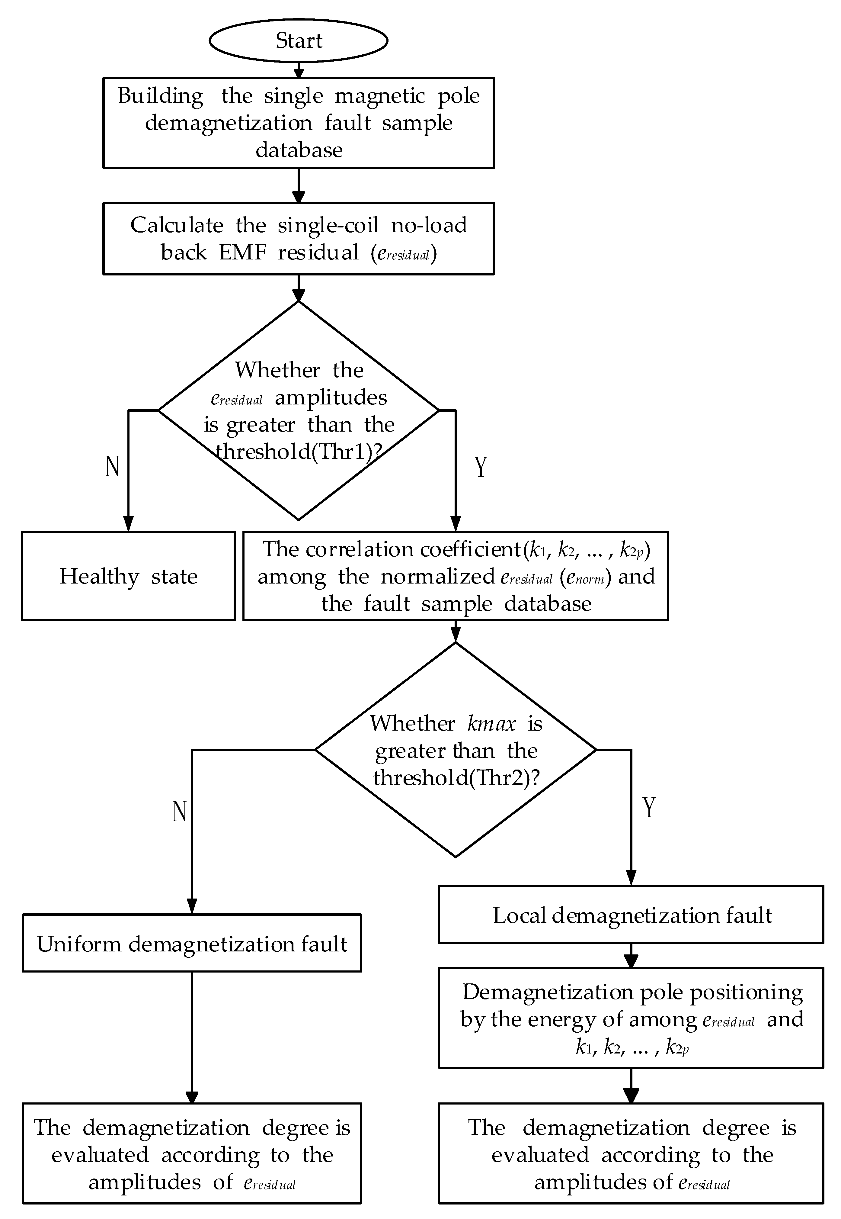
Figure 4.
Extraction process of demagnetization fault eigenvector: (a) the waveform of single-coil no-load back EMF under healthy state and demagnetizing fault; (b) the waveform of eresidual under demagnetizing fault.
Figure 4.
Extraction process of demagnetization fault eigenvector: (a) the waveform of single-coil no-load back EMF under healthy state and demagnetizing fault; (b) the waveform of eresidual under demagnetizing fault.
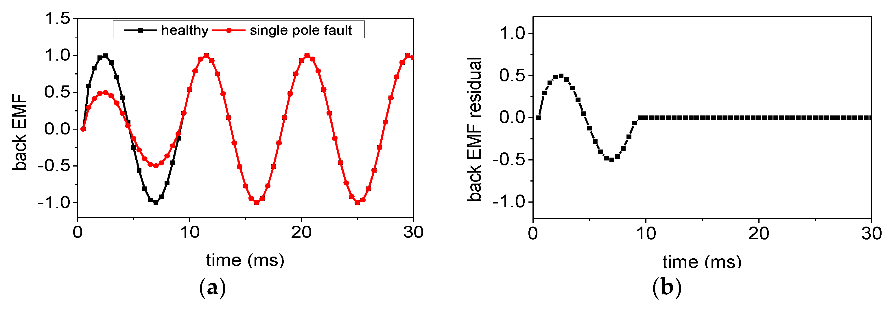
Figure 5.
Demagnetization fault characteristic quantity waveform.

Figure 6.
The eresidual waveform of different degree demagnetization fault.
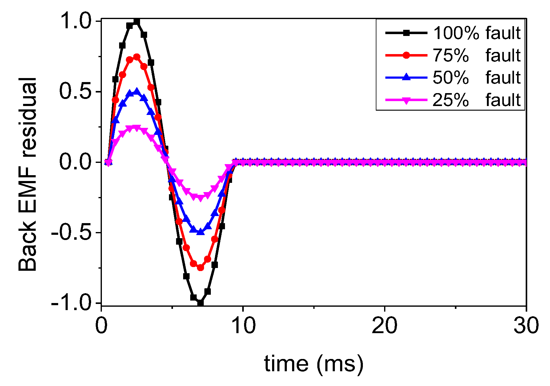
Figure 7.
eresidual under healthy, uniform demagnetization fault, and local demagnetization fault.
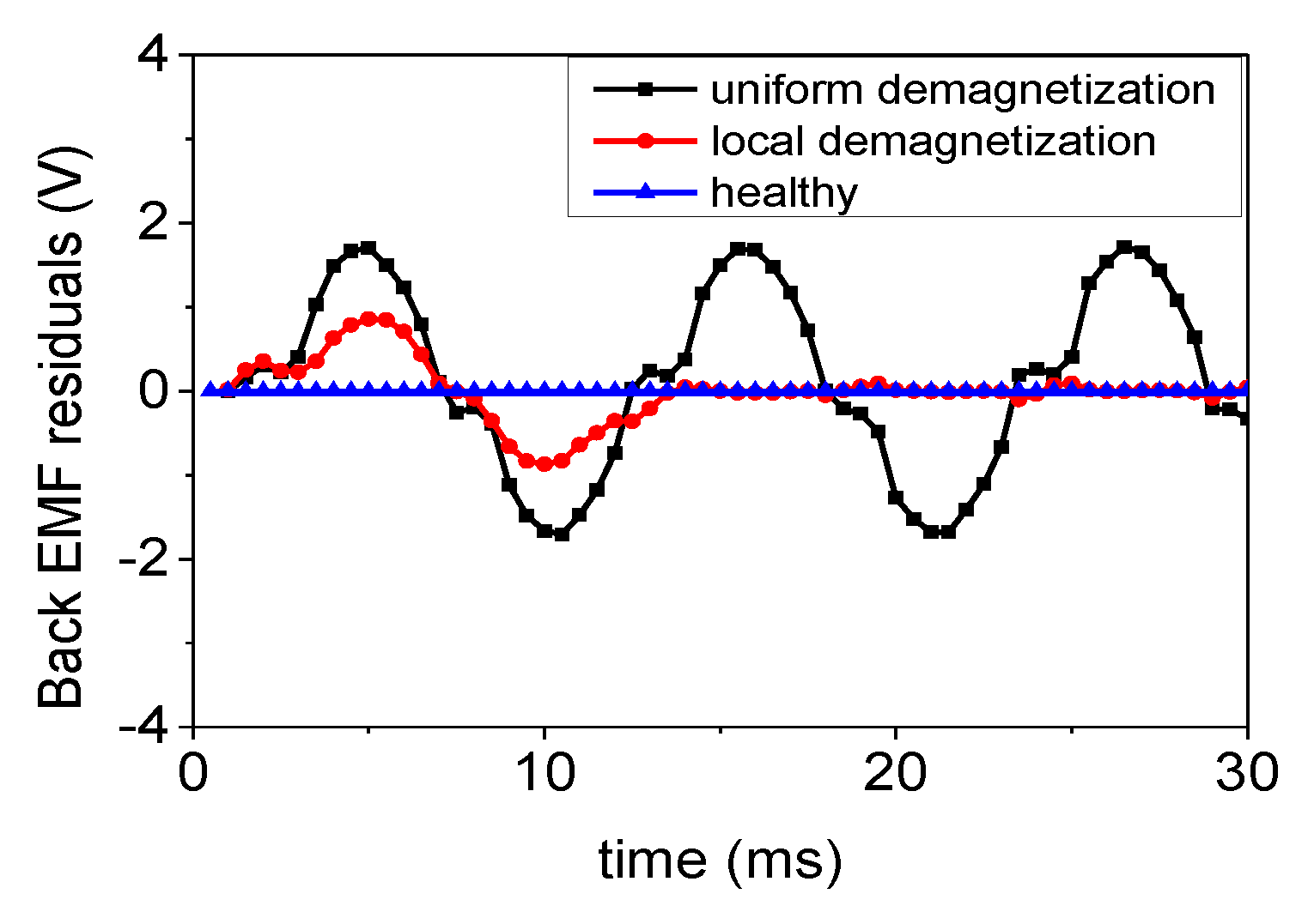
Figure 8.
The single-coil no-load back EMF residual with different degrees of demagnetization fault: (a) uniform demagnetization fault; (b) single pole demagnetization fault.
Figure 8.
The single-coil no-load back EMF residual with different degrees of demagnetization fault: (a) uniform demagnetization fault; (b) single pole demagnetization fault.
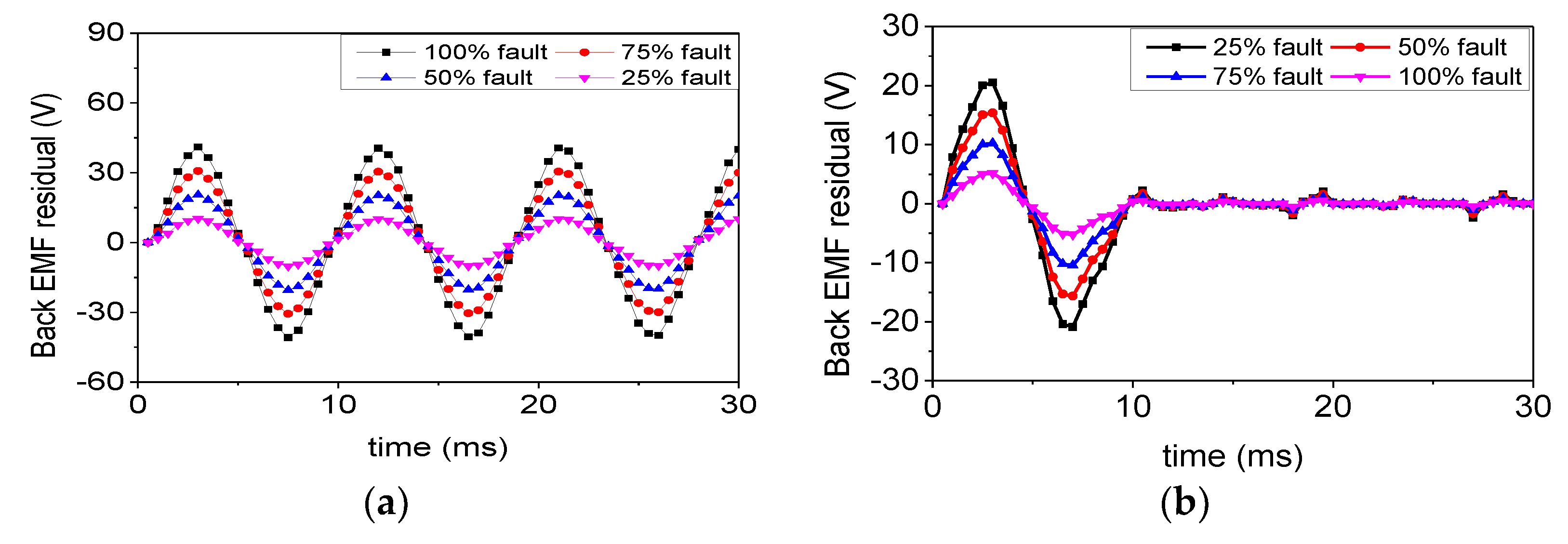
Figure 9.
The relationship between demagnetization degree and the peak of the single-coil no-load back EMF residual: (a) uniform demagnetization fault; (b) single pole demagnetization fault.
Figure 9.
The relationship between demagnetization degree and the peak of the single-coil no-load back EMF residual: (a) uniform demagnetization fault; (b) single pole demagnetization fault.


Table 1.
The key parameters of the PMSM.
| Items | Values | Unit |
|---|---|---|
| Out diameter of stator | 360 | mm |
| Inner diameter of stator | 300 | mm |
| Air-gap length | 1.2 | mm |
| Wire diameter of winding | 1.3 | mm |
| Area of slot | 154 | mm2 |
| Thickness of PM | 5.3 | mm |
| Angle of PM | 5 | ° |
| Axial length | 150 | mm |
| Rated power | 10 | kW |
| Rated speed | 200 | r/min |
| Number of phases | 3 | - |
| Number of coils | 36 | |
| Coil turn | 48 | |
| Parallel-circuits per phase | 3 | |
| Slot-Pole combination | 72–66 |
Table 2.
Correlation coefficients between the enorm of uniform demagnetization fault and fault sample database.
Table 2.
Correlation coefficients between the enorm of uniform demagnetization fault and fault sample database.
| Sample Characteristic Quantity Numbered | Uniform Demagnetization Fault Degree | |
|---|---|---|
| Fault 25% | Fault 75% | |
| 1 | 0.1748 | 0.1747 |
| 2 | 0.1749 | 0.1749 |
| 3 | 0.1749 | 0.1748 |
| 4 | 0.1746 | 0.1746 |
| 5 | 0.1749 | 0.1745 |
| 6 | 0.1741 | 0.1743 |
| 7 | 0.1740 | 0.1746 |
| 8 | 0.1742 | 0.1741 |
| … | … | … |
| 2p | 0.1747 | 0.1746 |
Table 3.
Correlation coefficients between the enorm of single Pole 2 demagnetization fault and fault sample database.
Table 3.
Correlation coefficients between the enorm of single Pole 2 demagnetization fault and fault sample database.
| Sample Characteristic Quantity Numbered | Local Demagnetization Fault Degree | |
|---|---|---|
| Fault 25% | Fault 75% | |
| 1 | 0.5 | 0.5 |
| 2 | 1 | 1 |
| 3 | 0.5 | 0.5 |
| 4 | −2.1972 × 10⁻⁸ | -2.1982 × 10⁻⁸ |
| 5 | 9.9593 × 10⁻¹¹ | 9.9571 × 10⁻¹¹ |
| 6 | 1.1050 × 10⁻¹⁰ | 1.1140 × 10⁻¹⁰ |
| 7 | 1.1051 × 10⁻¹⁰ | 1.1041 × 10⁻¹⁰ |
| 8 | 9.8452 × 10⁻¹¹ | 9.8471 × 10⁻¹¹ |
| … | … | … |
| 2p | 1.1131 × 10⁻¹⁰ | 1.1067 × 10⁻¹⁰ |
Table 4.
Correlation coefficients between uniform demagnetization with different degrees and fault sample database.
Table 4.
Correlation coefficients between uniform demagnetization with different degrees and fault sample database.
| Sample Characteristic Quantity Numbered | Uniform Demagnetization Fault Degree | |||
|---|---|---|---|---|
| Fault 12.5% | Fault 25% | Fault 50% | Fault 75% | |
| 1 | 0.1952 | 0.1952 | 0.1952 | 0.1952 |
| 2 | 0.1952 | 0.1952 | 0.1952 | 0.1952 |
| 3 | 0.1954 | 0.1954 | 0.1954 | 0.1954 |
| 4 | 0.1951 | 0.1951 | 0.1951 | 0.1951 |
| 5 | 0.1951 | 0.1951 | 0.1951 | 0.1951 |
| 6 | 0.1954 | 0.1954 | 0.1954 | 0.1954 |
Table 5.
Correlation coefficients between single pole 2 with different demagnetization degrees and fault sample database.
Table 5.
Correlation coefficients between single pole 2 with different demagnetization degrees and fault sample database.
| Sample Characteristic Quantity Numbered | Local Demagnetization Fault Degree | |||
|---|---|---|---|---|
| Fault 12.5% | Fault 25% | Fault 50% | Fault 75% | |
| 1 | 0.4413 | 0.4492 | 0.4566 | 0.4613 |
| 2 | 0.9924 | 0.9958 | 0.9984 | 0.9996 |
| 3 | 0.4446 | 0.4474 | 0.4522 | 0.4567 |
| 4 | 0.0166 | 0.0187 | 0.0243 | 0.0289 |
| 5 | 0.0019 | 0.0005 | 0.0057 | 0.0104 |
| 6 | 0.0285 | 0.0299 | 0.0337 | 0.0375 |
Table 6.
The energy of the single-coil no-load back EMF residual with different numbers of demagnetization poles.
Table 6.
The energy of the single-coil no-load back EMF residual with different numbers of demagnetization poles.
| One Pole Fault | Two Pole Fault | Three Pole Fault | |||
|---|---|---|---|---|---|
| Fault Pole | Energy | Fault Pole | Energy | Fault Pole | Energy |
| 1 | 697 | 1, 2 | 1990 | 1, 2, 3 | 3276 |
| 2 | 699 | 1, 3 | 1433 | 1, 2, 4 | 2711 |
| 3 | 703 | 1, 4 | 1406 | 1, 3, 4 | 2700 |
| 4 | 699 | 1, 5 | 1458 | 1, 2, 5 | 2687 |
| 5 | 703 | 1, 6 | 1407 | 1, 3, 5 | 2273 |
| 6 | 699 | 2, 3 | 1995 | 2, 3, 4 | 3280 |
Table 7.
Correlation coefficients between demagnetization fault and fault sample database.
| Sample Characteristic Quantity Numbered | Demagnetization Magnetic Pole Numbered | |||||||||||
|---|---|---|---|---|---|---|---|---|---|---|---|---|
| One Pole Fault | Two Pole Fault | Three Pole Fault | ||||||||||
| 1 | 2 | 3 | 4 | 5 | 6 | 1, 2 | 1, 3 | 2, 3 | 1, 2, 3 | 1, 2, 4 | 1, 3, 5 | |
| 1 | 0.9924 | 0.4651 | 0.0308 | 0.0170 | 0.0384 | 0.0130 | 0.8519 | 0.7215 | 0.2749 | 0.6735 | 0.7410 | 0.6023 |
| 2 | 0.4651 | 0.9958 | 0.4638 | 0.0335 | 0.0152 | 0.0415 | 0.8525 | 0.6333 | 0.8471 | 0.8684 | 0.7504 | 0.5113 |
| 3 | 0.0308 | 0.4638 | 0.9901 | 0.4661 | 0.0300 | 0.0178 | 0.2721 | 0.7052 | 0.8564 | 0.6702 | 0.4709 | 0.5684 |
| 4 | 0.0170 | 0.0335 | 0.4661 | 0.9988 | 0.4632 | 0.0338 | 0.0037 | 0.3536 | 0.2737 | 0.2176 | 0.5095 | 0.5136 |
| 5 | 0.0384 | 0.0152 | 0.0300 | 0.4632 | 0.9996 | 0.4641 | 0.0126 | 0.0743 | 0.0018 | 0.0218 | 0.2461 | 0.5837 |
| 6 | 0.0130 | 0.0415 | 0.0178 | 0.0338 | 0.4641 | 0.9927 | 0.0107 | 0.0425 | 0.0137 | 0.0157 | 0.0264 | 0.3128 |
Table 8.
Comparison of evaluation value and FEM results of uniform demagnetization.
| FEM Simulation Value | 0 | 25% | 50% | 75% | 100% |
|---|---|---|---|---|---|
| evaluation value | 0 | 25.01% | 50.00% | 74.99% | 100% |
Table 9.
Comparison of evaluation value and FEM results of single pole demagnetization fault.
| FEM Simulation Value | 0 | 25% | 50% | 75% | 100% |
|---|---|---|---|---|---|
| evaluation value | 0 | 25.02% | 50.03% | 74.97% | 100% |
© 2019 by the authors. Licensee MDPI, Basel, Switzerland. This article is an open access article distributed under the terms and conditions of the Creative Commons Attribution (CC BY) license (http://creativecommons.org/licenses/by/4.0/).
Share and Cite
MDPI and ACS Style
Gao, C.; Nie, Y.; Si, J.; Fu, Z.; Feng, H. Mode Recognition and Fault Positioning of Permanent Magnet Demagnetization for PMSM. Energies 2019, 12, 1644. https://doi.org/10.3390/en12091644
AMA Style
Gao C, Nie Y, Si J, Fu Z, Feng H. Mode Recognition and Fault Positioning of Permanent Magnet Demagnetization for PMSM. Energies. 2019; 12(9):1644. https://doi.org/10.3390/en12091644
Chicago/Turabian StyleGao, Caixia, Yanjie Nie, Jikai Si, Ziyi Fu, and Haichao Feng. 2019. "Mode Recognition and Fault Positioning of Permanent Magnet Demagnetization for PMSM" Energies 12, no. 9: 1644. https://doi.org/10.3390/en12091644
Note that from the first issue of 2016, this journal uses article numbers instead of page numbers. See further details here.