Demand Response Optimization Using Particle Swarm Algorithm Considering Optimum Battery Energy Storage Schedule in a Residential House

Abstract

Demand response as a distributed resource has proved its significant potential for power systems. It is capable of providing flexibility that, in some cases, can be an advantage to suppress the unpredictability of distributed generation. The ability for participating in demand response programs for small or medium facilities has been limited; with the new policy regulations this limitation might be overstated. The prosumers are a new entity that is considered both as producers and consumers of electricity, which can provide excess production to the grid. Moreover, the decision-making in facilities with different generation resources, energy storage systems, and demand flexibility becomes more complex according to the number of considered variables. This paper proposes a demand response optimization methodology for application in a generic residential house. In this model, the users are able to perform actions of demand response in their facilities without any contracts with demand response service providers. The model considers the facilities that have the required devices to carry out the demand response actions. The photovoltaic generation, the available storage capacity, and the flexibility of the loads are used as the resources to find the optimal scheduling of minimal operating costs. The presented results are obtained using a particle swarm optimization and compared with a deterministic resolution in order to prove the performance of the model. The results show that the use of demand response can reduce the operational daily cost.

1. Introduction

The future of power systems has been guided of a new structure where consumers (end-users) are considered as a central entity. This vision is presented in the Strategic Energy Technology (SET) plan of the European Union [1]. The transformation of end-users’ roles allows these entities to have an active contribution in electric power systems. The prosumer is a new concept that has its origin in the proliferation of Distributed Generation (DG) in end-user facilities. The Prosumer definition is presented in Reference [2], where prosumers are considered agents that can either consume or produce energy. The integration of renewable energy sources (RESs) and energy storage systems results in the increase the complexity of energy management. In Reference [3], some methods to optimize renewable energy systems management are revised.

Regarding demand response (DR) programs, the potential for participation in facilities is significantly increased by the distributed energy resources and especially the energy storage systems. With the participation in DR programs, the roles of the consumers change from a passive entity to an active entity that manages both local consumption and generation resources [4]. DR constitutes a modification of load profile in response to monetary or price signals, and thus provides flexibility and aims to help power systems during peak hours of demand or contingencies cases [5]. As the DR programs are able to reschedule part of the load, the use of these programs is a way to increase the flexibility of the grid management, avoiding the need to invest in more capacity [6].

Categorizing DR programs, it can be divided into two main categories: incentive-based DR programs and price-based DR programs. The incentive-based DR programs are referred to as the first category for DR programs, where the consumers can offer an incentive to change their consumption patterns. Direct load control programs, load curtailment programs, demand bidding programs, and emergency demand reduction programs are examples of incentive-based DR programs. The “price-based DR programs” are the second category of DR programs, where the consumers are charged with different rates at different consumptions times. Therefore, the retail electricity tariff is affected by the cost of electricity supply. The price-based DR programs types are a time of use pricing, critical peak pricing, real-time pricing, and inclining block rate [7]. Advanced infrastructure metering is needed to implement DR programs at the residential, commercial, or industrial level. Such infrastructure (i.e., smart meters) is able to measure and store energy utilization at different times and also obtain the current usage information remotely.

The European Union has shown significant interest in the concept of smart metering. According to [8], it is expected by 2020 to invest ~45 million euros for 200 million smart electricity meters and 45 million smart meters of natural gas. This facilitates the application of DR programs in most electrical facilities.

Regarding the formulation of DR optimization problems, linear programming (LP) or nonlinear programming (NLP) can be used. Frequently the DR problems are able to use binary decision variables for determining the status (ON or OFF) of various consumers or appliances; in these situations, mixed-integer linear programming (MILP) or mixed-integer nonlinear programming (MINLP) may be used. In Reference [9], the authors use MILP to optimize DR and generate scheduling in a residential community grid using renewable energies, batteries, and electric vehicles. In this optimization, a minimization problem of purchased energy costs of the residential community has been solved. In Reference [10] a cost minimization in smart building microgrid considering DR optimization and day-ahead operation is implemented using MILP. This case study is composed of two different smart buildings with 30 and 90 houses. During the optimization process, the optimal schedule of house appliances is found. Another MILP approach is applied in Reference [11], showing how strategies like DR can achieve suitability in any region considering the presence of high penetration of renewable-based generation.

An example of NLP applied for DR optimization is presented in Reference [12], where the unit commitment problem for a microgrid is solved. The optimization problem finds the amount of load reduction and paid incentives for each time interval. Another example of MINLP has been presented in Reference [13], which considers the minimization of purchase gas and electricity from the grid by including the consumption of different loads at different periods. The optimal day-ahead scheduling of resources in energy hubs is determined.

The DR application in end consumers has been over time applied through an aggregator. It works as a service provider, and the DR services must be paid to this provider. In Reference [14], an aggregation of thermostatically controlled loads for performing DR is presented. In this case, the air conditioning consumption is considered as the load. The aggregation services are not restricted to the application of DR programs, in Reference [15] an aggregation of generalized energy storage can be found. The aggregator storage is used to participate in the energy and regulation market. DR programs targeting independent users, without the need of contracts or service providers, are also possible [16,17]. These applications are considered independent because the user is not connected to any aggregator. Usually, when the application is independent the user has a device installed in its house to control the loads. In Reference [16], the controller is a PV inverter, while in Reference [17], a home energy management system is used. The controllable loads can be divided into passive (i.e., air conditioning, fridges, washing machine) and active (i.e., DG, ESS, vehicle-to-grid, PV) loads [18]. In References [16,19] the DR is applied on discrete loads, which only have two states: on or off.

With focus on artificial intelligence (AI), its application in power systems has increased in the past years. The metaheuristics are a very popular part of AI for solving optimization problems. These techniques have acceptable performance in order to solve engineering problems by finding a near-optimal solution with a limited computation burden. Metaheuristics can be applied in problems with a large number of decision variables and easily adapted to a problem that has several constraints [20]. A PSO variant is used in Reference [17] for finding the optimal operation of price-driven demand response with a load shifting dispatch strategy for photovoltaic, storage battery, and power grid systems. The optimization algorithm is implemented on Home Energy Manage System. In Reference [21], the PSO algorithm is also used. The DR is optimized considering the variation of electricity price imposed by DSO to provoke a consumption reduction. In the microgrid environment [22], a PSO is used for solve the DR optimization problem. In this case a dynamic pricing model is considered for increase the profit of costumers. In Reference [23] a PSO algorithm is proposed to optimize the performance of a smart microgrid in a short term to minimize operating costs and emissions. Other algorithms like genetic algorithm [24], simulated annealing [25], and differential evolution [26] are frequently used algorithms to solve DR optimization problems.

The present paper proposes DR optimization considering the optimal battery schedule in a residential house with Photovoltaic (PV) generation. A PSO approach is implemented to solve the optimization problem (MILP), and the results are compared with a deterministic resolution (CPLEX solver). The consumer (residential house) is provided with independent management that approaches the several resources capabilities and contributions for the minimization of energy bought from the grid. The main contributions of this paper are as follows.

(1)

To perform DR without any contract with the DR service provider—this presented methodology allows the user to perform DR actions without any connection with DR services provider. The consumer is provided with independent management that approaches the several resources capabilities and contributions for the minimization of bought energy from the grid.

(2)

The implementation of PSO which is a very simple metaheuristic to implement, open access, multiplatform (Windows, MacOS, Linux, etc.), executable from an Arduino/Raspberry and also is the cheapest implementation option. Referring to the presented solution in [16], which uses a CPLEX solver for MATLAB/TOMLAB platform, the implementation of the PSO is a much affordable solution, once that MATLAB and TOMLAB are non-open access. PSO can be implemented in an open access environment and can be executed in free simple platforms, such as Python.

(3)

The proposed methodology represents an optimization problem that can considerably improve the consumer’s energy savings—the combined use of resources (PV production, storage capacity, and loads flexibility) allows for a significant reduction in daily operation costs. The optimal solution obtained by PSO has a daily cost of 3.28 €, while an operation without PV production, storage capacity and loads flexibility has a cost of 16.83 € per day, which is five times higher than PSO result for best scenario. If one considers a base scenario that was obtained by using a simple management mechanism considering the PV production and storage capacity, the daily cost is 9.33 €, which is three times higher than PSO result for the best scenario. The assessment of PSO can be verified in the comparison of the base scenario and the optimized base scenario with the PSO. The daily costs with PSO decreases 1.38 €.

The paper is structured into seven sections: In Section 1 an introduction about DR and how to solve DR problems is presented. Section 2 presents the proposed methodology; in Section 3 the problem formulation is presented. Section 4 presents the algorithm (PSO) and its adaptation to the problem formulation. In Section 5, the case study is presented as well as all input variables and PSO parameters. Section 6 presents the results, and the conclusions are presented in Section 7.

2. Proposed Methodology

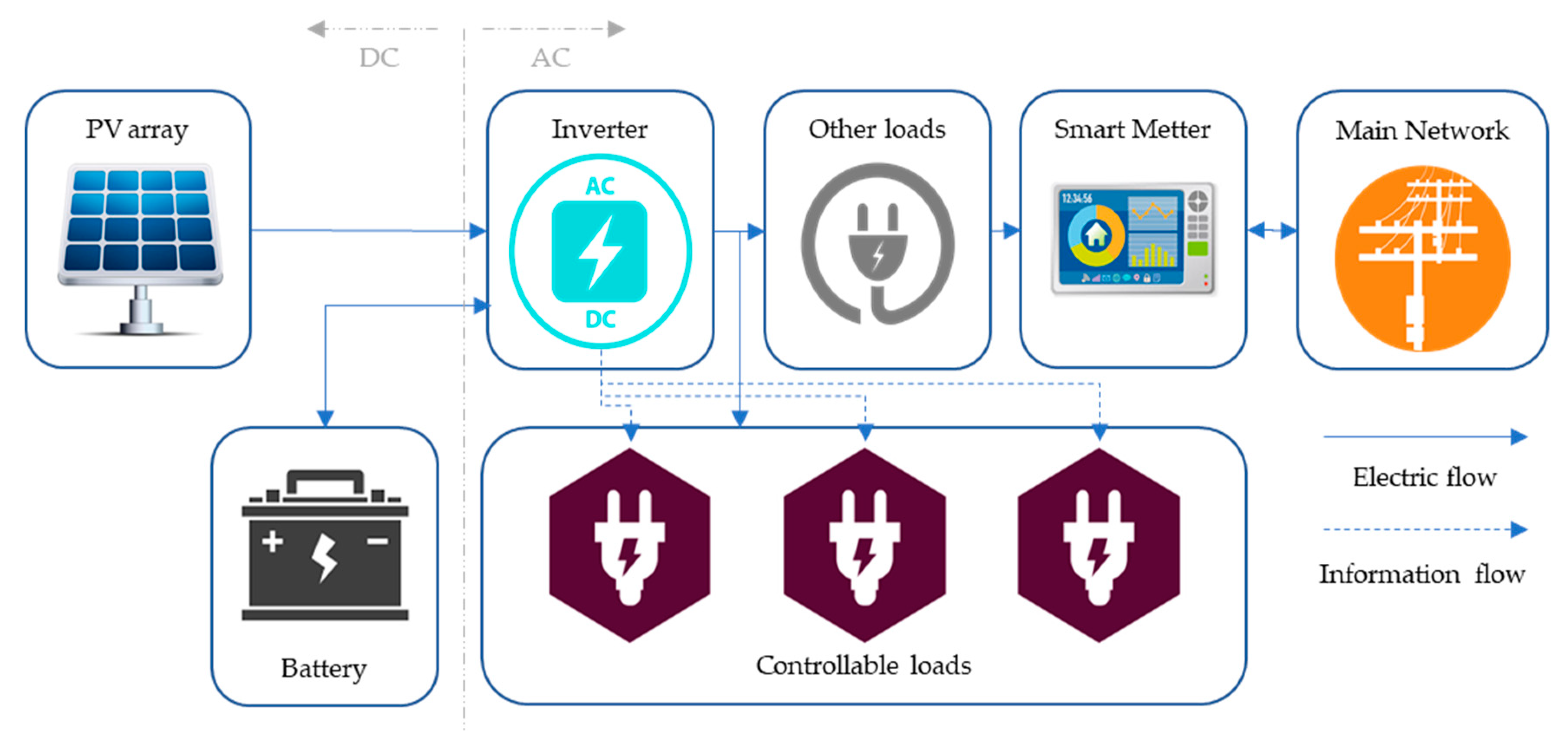
With the goal to reduce the electricity bill of the end consumers is introduced the presented methodology. This methodology aims to minimize the operation costs considering the batteries and flexibility provided by the DR actions. The costs minimization considered the grid, the PV systems, energy storage batteries, and consumption flexibility through load scheduling. The end consumer is connected to the grid, and has a tariff contract that allows selling energy in the grid in exchange for monetary payment. This methodology is able to be expanded to other consumers with different conditions and with different numbers of resources. Figure 1 presents the context scheme of the idea proposed. This scheme is typical for a household prosumer. The scheme of Figure 1 has a unit generation (PV), energy storage system (ESS) (battery), one inverter module, the controllable and noncontrollable loads, and a smart meter.

For household, the use of PV generation is considered free (the generation unit is household property). In this paper, the PV generation is considered priority above all others, meaning that when it is available it will always be used either by load’s necessities, battery charge, or injection in the grid. The connection with the grid is considered bidirectional. The PV rated power is usually limited by a contract between retailer and household. This limitation occurs because it can be a source of problems for the physical grid. In this way, it is difficult to reach a situation in which, as limit case if no injection to the grid is allowed, the PV is higher than the load plus the energy that can be used to charge the battery. However, if it happens, the inverter will disconnect the PV in order to avoid overvoltage. In Figure 1 one can see power flows and information flows. The information flows are connected to the inverter and controllable loads. In this case, the inverter is enabled with a control and management system that allows controlling loads, adding DR actions in household installation.

In general, the consumer can take advantage of the use of PV generation, ESS, and DR actions to minimize the cost of consumption from the grid. The consumer can look for the periods where electricity is cheaper to satisfy the consumption and charge the ESS, and the periods where the electricity price is most expensive to sell the excess electricity from the facility. Thus, it can be considered as a management system for the consumer to improve his energy bill.

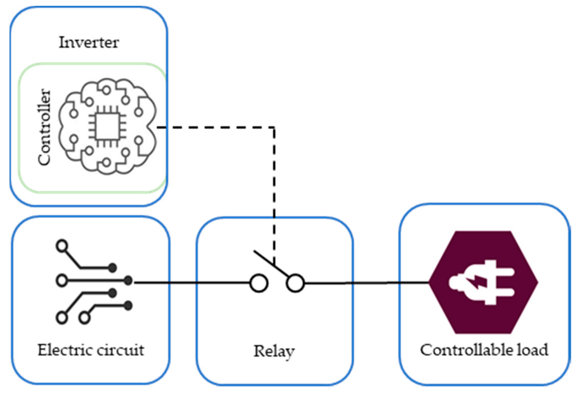
Figure 2 is a representative illustration of the load’s control using relays. The controller, in this case, is a component of the inverter. Each controllable load must have one relay associated with it, which allows for its control. So, when the controller sends the signal to the relay, the load is connected or disconnected from the electrical circuit. In this case, this control is considered a DR cut (direct load control). The scheme in Figure 2 considers only one relay for simplification; however, the proposed methodology is able to consider several relays, one for each load in the facility.

3. Problem Formulation

The mathematical formulation is presented throughout this section. With the formulation presented it is intended to simulate the interaction of a consumer with the grid. The main goal is to minimize the operation costs, considering that the user has storage units and is also enabled to do DR in specific loads. The presented optimization model is considered a mixed-integer linear problem. Equation (1) presents the objective function.

$$Minimize f=Energy Bill+DR Curtailment$$

(1)

Equation (1) is comprised of the sum of two different parcels: the energy bill present in Equation (2) and the DR curtailment present in Equation (3). The Energy Bill represents the cost of buying and selling energy, and the DR curtailment refers to cost weighting associated with kWh curtailment.

In Equation (2) the variable $P_t^{grid}$ represents the flow of energy between household and grid, $I_t^{grid in}$ is an indicator variable for power flow into the grid and control the energy buy $\left(I_t^{grid in}=1\right)$ and energy sell $\left(I_t^{grid in}=0\right)$, $C_t^{grid in}$ represents the cost of buying electricity and $C_t^{grid out}$ represents the cost of selling electricity. The Energy bill in Equation (2), consider the costs of buying electricity $\left(I_t^{grid in}\times P_t^{grid}\right)\times C_t^{grid in}$ and the revenues of selling electricity $\left(\left(1-I_t^{grid in}\right)\times P_t^{grid}\right)\times C_t^{grid out}$. In each period $\left(t\right)$ the user can make a single operation (buy or sell).

$$Energy Bill={\displaystyle \sum }_{t=1}^T\left[\left(\left(I_t^{grid in}\times P_t^{grid}\right)\times C_t^{grid in}-\left(\left(1-I_t^{grid in}\right)\times P_t^{grid}\right)\times C_t^{grid out}\right)\times \frac{1}{\Delta t}\right]+DCP$$

(2)

$$I_t^{grid in}=\{\begin{array}{l}1,\hspace{1em}\hspace{1em}if P_t^{grid}>0\\ 0,\hspace{1em}\hspace{1em}otherwise\end{array} \forall t\in \left\{1,\dots ,T\right\}$$

Also, in Equation (2) the term $\left(\left(1-I_t^{grid in}\right)\times P_t^{grid}\right)$ represents the power sent to the network. The term $\Delta t$ is used for to adjust the consumption to the tariff price because normally the tariff is available in €/kWh and the optimization can be scheduled at different time intervals (e.g., 15 min). $DCP$ represents the daily contracted power cost. If the term $P_t^{grid}$ has a positive value during optimization it means that there is electricity consumption from the network. However, if it has a negative value it means that there is a sale of electricity to the network. Equation (3) presents the DR curtailment.

$$DR Curtailment={\displaystyle \sum }_{t=1}^T\left({\displaystyle \sum }_{l=1}^L{P}_{l,t}^{cut}\times X_{l,t}^{cut}\times W_{l,t}^{cut}\right)$$

(3)

If the DR curtailment equation is implemented the cost of load is cut with the use of weights, and in fact does not have cost for the user. The variable $P_{l,t}^{cut}$ represents the cut energy of load $\left(l\right)$ in period $\left(t\right)$, the $X_{l,t}^{cut}$ represents the decision binary variable to active the cut of load $\left(l\right)$ in period $\left(t\right)$, and $W_{l,t}^{cut}$ represents the cut weight of load $\left(l\right)$ in period $\left(t\right)$. The term $\left(P_{l,t}^{cut}\times X_{l,t}^{cut}\times W_{l,t}^{cut}\right)$ shows the interest of the user to perform cut in load $\left(l\right)$ in period $\left(t\right)$.

Equation (4) represents the balance between load and generation, $P_{b,t}^{bat}$ represents the energy charged or discharged by baterry $\left(b\right)$ in period $\left(t\right)$. If the value of $P_{b,t}^{bat}$ is less than 0 the battery is discharging, otherwise, if the value of $P_{b,t}^{bat}$ is greater than 0, the battery is charging. The variable $P_{p,t}^{PV}$ represents the photovoltaic production of unit $p$ at period $t$, and $P_t^{load}$ corresponds to the value of load at period $t$.

$$P_t^{grid}=P_t^{load}+{\displaystyle \sum }_{b=1}^B{P}_{b,t}^{bat}-{\displaystyle \sum }_{l=1}^L{P}_{l,t}^{cut}\times X_{l,t}^{cut}-{\displaystyle \sum }_{p=1}^P{P}_{p,t}^{PV},\hspace{1em}\hspace{1em}\forall t\in \left\{1,\dots ,T\right\}$$

(4)

The Equation (5) shows the balance of battery systems.

$$E_{b,t}^{stor}=E_{b,t-1}^{stor}+P_{b,t}^{bat}\times \frac{1}{\Delta t},\hspace{1em}\hspace{1em}\forall t\in \left\{2,\dots T\right\}, \forall b\in \left\{1,\dots ,B\right\}$$

(5)

Variable $E_{b,t}^{stor}$ represents the state of the battery $b$ in period $t$, in other words, it represents the amount of energy it has available. So, by Equation (5) the current battery state is obtained by adding the previous state $E_{b,t-1}^{stor}$ to the value of the variable $P_{b,t}^{bat}$.The power term $P_{b,t}^{bat}$ in Equation (5) is multiplied by $\frac{1}{\Delta t}$ to convert power into energy units. The system is governed by the following constraints (Equations (6)–(10)).

$$-P_t^{grid min}\le P_t^{grid}\le P_t^{grid max}\hspace{1em}\hspace{1em}\forall t\in \left\{1,\dots ,T\right\}$$

(6)

$$P_{l,t}^{cut}=P_{l,t}^{cut max}\hspace{1em}\hspace{1em}\forall l\in \left\{1,\dots ,L\right\}, \forall t\in \left\{1,\dots ,T\right\}$$

(7)

$$0\le E_{b,t}^{stor}\le E_{b,t}^{stor max}\hspace{1em}\hspace{1em}\forall b\in \left\{1,\dots ,B\right\}, \forall t\in \left\{1,\dots ,T\right\}$$

(8)

$$-P_{b,t}^{dch max}\le P_{b,t}^{bat}\le P_{b,t}^{ch max}\hspace{1em}\hspace{1em}\forall b\in \left\{1,\dots ,B\right\}, \forall t\in \left\{1,\dots ,T\right\}$$

(9)

$$X_{l,t}^{cut}=\{\begin{array}{l}1\\ 0\end{array}\hspace{1em}\hspace{1em}\forall l\in \left\{1,\dots ,L\right\}, \forall t\in \left\{1,\dots ,T\right\}.$$

(10)

In Equation (6), the variable $P_t^{grid min}$ and $P_t^{grid max}$ represent the limit values for variable $P_t^{grid}$. Equation (7) identifies that $P_{l,t}^{cut}$ can only take the maximum value $P_{l,t}^{cut max}$. The $P_{b,t}^{bat}$ variables can take a value between $-P_{b,t}^{dch max}$ and $P_{b,t}^{ch max}$; if the value of $P_{b,t}^{bat}$ is less than zero it represents a discharge and if the value is greater than zero it represents a charge. The variable $X_{l,t}^{cut}$ is a binary variable and represents a decision variable. When $X_{l,t}^{cut}$ is equal to 1 the cut of load ($l)$ at period $\left(t\right)$ is active.

4. Particle Swarm Optimization

PSO was proposed by Kennedy and Eberhart in 1995, and it is a random search algorithm that simulates the foraging and flocking of birds in nature [27]. When birds look randomly for food in a given area, each bird can be associated with a single solution and can be considered as a particle in the swarm.

For PSO implementations assume that it has $j$ particles in the n-dimensional search space and each particle represent a solution in the search space. Equation (11) presents the position vector of particle j and in Equation (12) the velocity vector for particle j.

$${\overrightarrow{x}}_i^j=\left(x_{i,1}^j,x_{i,2}^j,\dots ,x_{i,n}^j\right)$$

(11)

$${\overrightarrow{v}}_i^j=\left(v_{i,1}^j,v_{i,2}^j,\dots ,v_{i,n}^j\right)$$

(12)

where, ${\overrightarrow{x}}_i^j$. represents the position vector of particle $j$ for $n$. variables at iteration $i$. The ${\overrightarrow{v}}_i^j$ represents the velocity vector of particle $j$ for n variables. When the search process starts, both vectors are generated randomly between the respective limits of the n variables.

Equation (13) represents the velocity update equation. This equation is composed of three different components: the $w_i^j{\overrightarrow{v}}_i^j$ component represents the previous positions in memory search, $c{1}_i^{j}r{1}_i^j\left(P_{best}^j-{\overrightarrow{x}}_i^j\right)$ corresponds to the cognitive learning component, and $c{2}_i^{j}r{2}_i^j\left(G_{best}-{\overrightarrow{x}}_i^j\right)$ is a global learning component. Equation (14) represents the position update.

$${\overrightarrow{v}}_{i+1}^j=w_i^j\times {\overrightarrow{v}}_i^j+c{1}_i^j\times r{1}_i^j\times \left(P_{best}^j-{\overrightarrow{x}}_i^j\right)+c{2}_i^j\times r{2}_i^j\times \left(G_{best}-{\overrightarrow{x}}_i^j\right)$$

(13)

$${\overrightarrow{x}}_{i+1}^j={\overrightarrow{v}}_{i+1}^j+{\overrightarrow{x}}_i^j$$

(14)

where, ${\overrightarrow{v}}_{i+1}^j$ is the velocity vector at iteration $i+1$; $w_i^j$ represents the inertia weight obtained through Equation (15); $c{1}_i^j$ and $c{2}_i^j$ are acceleration coefficients, which are obtained by Equations (16) and (17), respectively; and $r{1}_i^j$ and $r{2}_i^j$ are two uniformly distributed random numbers independently generated within [0,1] for the n-dimensional search space. $P_{best}^j=\left(x_{pbest,1}^j,x_{pbest,2}^j,\dots ,x_{pbest,n}^j\right)$ denotes the historical best position and $G_{best}=\left(x_{gbest,1}, x_{gbest,2},\dots , x_{gbest,n}\right)$ denotes the population historical best position. Equation (15) presents an inertia weight.

$$w_i^j=w^{max}-\left(\frac{w^{max}-w^{min}}{i^{max}}\right)\times i$$

(15)

where, $w^{max}$ is the maximum value for inertia weight, $w^{min}$ is the minimum value for inertia weight, and $i^{max}$ represents the maximum value of iterations. The inertia weight present in Equation (15) is a linear decreasing method during the search process. The inertia weight reduction ensures strong global exploration properties in the initial phase and strong local exploitation properties in the advanced phase. The inertia weight is calculated at each iteration and is the same for the set of particles at each iteration [28]. Equations (16) and (17) present the acceleration coefficients calculation:

$$c{1}_i^j=c_1^{max}-\left(\frac{c_1^{max}-c_1^{min}}{i^{max}}\right)\times i$$

(16)

$$c{2}_i^j=c_2^{min}+\left(\frac{c_2^{max}-c_2^{min}}{i^{max}}\right)\times i$$

(17)

where, $c_1^{max}$ and $c_1^{min}$ are the maximum and minimum values for the personal acceleration coefficient, respectively. $c{1}_i^j$ decreases over the iterations, which means that the acceleration component for the personal position at the beginning of the search is high allowing exploration. The parameters $c_2^{min}$ and $c_2^{max}$ represent the minimum and maximum values for the global acceleration coefficient. $c{2}_i^j$ increases over the iterations, which means that the acceleration component for the global position at the end of the search is high allowing exploitation. The encoding of the solutions is crucial for the success of the algorithm. Equation (18) shows the encoded vector used for solving the problem present in Section 2.

$${\overrightarrow{x}}_i^j=\left[\left\{P_{1.1}^{bat},\dots , P_{B,T}^{bat}\right\},\left\{X_{1.1}^{cut},\dots , X_{L,T}^{cut}\right\}\right]$$

(18)

where, $\left\{P_{1.1}^{bat},\dots , P_{B,T}^{bat}\right\}$ is a group of continuous variables representing the electricity amount of charge or discharge in each battery ($b)$ at period $\left(t\right)$ and $\left\{X_{1.1}^{cut},\dots , X_{L,T}^{cut}\right\}$ are binary variables to enable the possibility of performed cut action in load $\left(l\right)$ at period $\left(t\right)$. Therefore, particle $\overrightarrow{x}$ has dimensions of $n=B\times T+L\times T$. This encoding allows a direct evaluation in Equation (1).

The PSO implementation starts by defining the search space limits by setting the lower and upper bounds of each variable. In Equation (19), $xl{b}^j$ represents the lower limits for the solution of $j$ particle and $xu{b}^j$ in Equation (20) represent the upper limit for $j$ particle.

$$xl{b}^j=\left[\left\{-P_{1.1}^{dch max},\dots , -P_{B,T}^{dch max}\right\},\left\{X_{1.1}^{cut min},\dots , X_{L,T}^{cut min}\right\}\right]$$

(19)

$$xu{b}^j=\left[\left\{P_{1.1}^{ch max},\dots , P_{B,T}^{ch max}\right\},\left\{X_{1.1}^{cut max},\dots , X_{L,T}^{cut min}\right\}\right]$$

(20)

$${\overrightarrow{x}}_1^j=rand \left[xl{b}^j,xu{b}^j\right]$$

(21)

Equation (21) presents the process of initialization where the initial solution was created. In this case, a random process into allowed bounds is executed. $rand \left[xl{b}^j,xu{b}^j\right]$ is a random number within the lower $xl{b}^j$ and the upper $xu{b}^j$ bounds of $j$ particle for $n$ variables.

Equation (22) presents the boundary constrains method. The search process over the iterations will generate new solutions that may not be within the initially stipulated limits. To address this issue the boundary control strategies are used to repair infeasible individuals. In this paper is used a boundary control technique known as bounce-back [20].

$${\overrightarrow{x}}_i^j=\{\begin{array}{l}\mathrm{rand}\left(xl{b}^j,{\overrightarrow{x}}_i^j\right)if{\overrightarrow{x}}_i^j<xl{b}^j\\ \mathrm{rand}\left({\overrightarrow{x}}_i^j,xu{b}^j\right)if{\overrightarrow{x}}_i^j>xu{b}^j\\ {\overrightarrow{x}}_i^j otherwise\end{array}$$

(22)

In contrast to random reinitialization (the most used control technique), bounce-back uses the information on the progress towards the optimum region by reinitialized the variable value between the base variable value and the bound being violated. Making use of domain knowledge about the problem, the Equations (23) and (24) is proposed as a direct repair equation. The Equation (23) concerns the direct repair of $E_{b,t}^{stor}$.

$$E_{b,t}^{stor}=\{\begin{array}{ll}\begin{array}{l}0\\ P_{b,t}^{ch max}\\ E_{b,t}^{stor}\end{array}& \begin{array}{l}if E_{b,t}^{stor}<0\\ if E_{b,t}^{stor}>E_{b,t}^{stor max}\\ otherwise \end{array}\end{array} \forall b\in \left\{1,\dots ,B\right\}, \forall t\in \left\{1,\dots ,T\right\}$$

(23)

Although boundary control is used it can only control the variables $P^{bat}$ and $X^{cut}$, the variable $E^{stor}$ is a variable of control and balance, and when it is repaired other variables are necessarily changed. For the repair process $E^{stor}$ is needed to test two different conditions, $E_{b,t}^{stor}<0$ represents a greater discharge than the allowed one, being that it fixes the variable to the minimum value. $E_{b,t}^{stor}>E_{b,t}^{stor max}$ means that the battery has a charge greater than the allowed, the value of maximum energy in the battery is fixed in maximum that can accumulate. Equation (24) presents the direct repair for $P^{bat}$ variable.

$$P_{b,t}^{bat}=\{\begin{array}{ll}\begin{array}{l}{E}_{b,t}^{stor}-E_{b,t-1}^{stor}\\ E_{b,t}^{stor}-E_{b,t-1}^{stor}\\ P_{b,t}^{bat}\end{array}& \begin{array}{l}if E_{b,t}^{stor}<0\\ if E_{b,t}^{stor}>E_{b,t}^{stor max}\\ otherwise \end{array}\end{array} \forall b\in \left\{1,\dots ,B\right\}, \forall t\in \left\{2,\dots ,T\right\}$$

(24)

$P^{bat}$ is repaired in Equation (22), but with the direct repair used in Equation (23) the variable $P^{bat}$ may not be correct, and it is necessary to perform direct repair on it. So, a battery power level test is performed, if $E_{b,t}^{stor}<0$ the value for $P_{b,t}^{bat}$ is equal to the difference between the battery power level in the previous period $E_{b,t-1}^{stor}$ and the current period $E_{b,t}^{stor}$. The same rule is applied when the battery power level is greater than the allowed maximum $E_{b,t}^{stor}>E_{b,t}^{stor max}$.

The particles should be evaluated according to a fitness function $f^{\prime }\left(\overrightarrow{x}\right)$, Equation (25), including objective function $f\left(\overrightarrow{x}\right)$ Equation (1) and constrains violation $pf\left(\overrightarrow{x}\right)$.

$$f^{\prime }\left(\overrightarrow{x}\right)=f\left(\overrightarrow{x}\right)+pf\left(\overrightarrow{x}\right)$$

(25)

$$pf\left(\overrightarrow{x}\right)=\{\begin{array}{l}{\displaystyle \sum _{t=1}^T}t\times \rho if P_t^{grid}\le P_t^{grid min}\cap P_t^{grid}\ge P_t^{grid max}\\ 0 otherwise\end{array} \forall t\in \left\{1,\dots ,T\right\}$$

(26)

where, $pf\left(\overrightarrow{x}\right)$ in Equation (26) represents the penalty value for a solution $\overrightarrow{x}$. Despite the application of bounce-back method Equation (22) and direct repair methods (23) and (24), the solution may still be infeasible. The penalty value is obtained checking the limits of variable $P_t^{grid}$ for every period. In each period that the variable is out of limit is counted and multiplied by a penalty amount $\rho$, the sum of all individual (per period) penalties represents the total penalties per each solution.

Pseudocode of the PSO algorithm is presented in Algorithm 1.

Algorithm 1. PSO pseudocode.

INITIALIZE Set control parameters $w^{max}$,$w^{min}$,$c_1^{max}$,$c_1^{min}$,$c_2^{max},$$c_2^{min}$, $j^{max}$, and $i^{max}$. Create an initial Pop (Equation (21)) and initial velocities. IF Direct repair is used THEN   Apply direct repair to unfeasible individuals END IF Evaluate the fitness of Pop (Equation (25)). Create a $P_{best}$ vector for every particle. Create $\mathrm{a} G_{best}$ vector of the swarm. FOR $i$ = 1 to $i^{max}$   FOR $j$ = 1 to $j^{max}$    Velocity update (Equation (13))    Position update (Equation (14))    Update $w_i$, $c{1}_i$ and $c{2}_i$ (Equations (15)–(17))    Verify boundary constraints for $P^{bat}$ (Equation (9))and $X^{cut}$ (Equation (10))    IF Boundary constraints are violated THEN      Apply boundary control (Equation (22))    END IF    Verify boundary constraints for $E^{stor}$ (Equation (8)) and $P^{bat}$ (Equation (9))    IF Boundary constraints are violated THEN      Apply direct repair (Equations (23) and (24))    END IF    Evaluate fitness of $\overrightarrow{x}$ (Equation (25)).    Verify boundary constraints for $P^{grid}$ (Equation (6))    IF $P^{grid}$ is out of limits THEN      Apply penalty function (Equation (26))      Update fitness value (Equation (25))    END IF    Update $P_{best}$ vector for $i$ particle.   END FOR   Update $G_{best}$ vector of the swarm. END FOR

Basically, if in the evaluation process constraints violations are identified, the individual is randomly repaired using the initialization process from Equation (22). The pseudocode of Algorithm 1 is displayed step-by-step, starts with the definition of the parameters related to the PSO. The search begins with the creation of the initial population. After being evaluated, the best position of each particle and the best position of the population are defined. The main cycle starts, and at each iteration of the main cycle, another cycle is performed for each particle. For each particle a new velocity is generated, updated, verified, and evaluated. When all particles repeat the process, the value of the best personal position of each particle and the best overall position of the population is updated.

5. Case Study

This section presents the case study. The optimization problem was solved using PSO metaheuristic and compared to a solution obtained by a CPLEX solver in MATLAB™/TOMSYM™ environment to compare the results.

The proposed methodology addresses a Portuguese consumer and complies with actual Portuguese legislation, which allows small producers (consumers with local generation) to use the energy produced to satisfy the own load necessities and sell it to the grid. The consumer has a supply power contract of 10.35 KVA with the retailer, and it is characterized by three different periods: peak, intermediate, and off-peak [29]. The prices applied to a consumer operation are present in

Table 1. Prices of the different periods and contracted power.

Parameter	Energy (€/kWh)			Contracted Power (€/Day)
	Peak	Intermediate	Off-Peak
Buy from grid	0.2738	0.1572	0.1038	0.5258
Periods	10.30 h–13 h 19.30 h–21 h	08 h–10.30 h 13 h–19.30 h, 21 h–22 h	22 h–02 h 02 h–08 h
Sell to grid	0.1659 *			−
DR weight	0	0.2	0.4

* is used for all periods.

. The input prices in Table 1 are real values of a Portuguese retailer (https://www.edp.pt/particulares/energia/tarifarios), which provides a realistic case study. The prosumer can inject his excess production into grid, but a limit is imposed by the retailer. The maximum value injected into grid is half of its contracted power, approximately 5.1 kW. The real prices and real condition inclusion in this problem contribute to more accurate in this study and prove the real value of the methodology application.

The DR weights present in Table 1 are defined by the consumer taking into account the energy price variation within the day, adapted from [16]. The use of DR is more appreciated when the energy is cheaper, so the weight of 0 is given in peak periods (highest price). With this weight distribution, the DR actions are expected to be executed during peak periods. Equation (3) gives the amount of DR actions contributing to the objective function. It does not represent costs for the consumer, but is rather a consumer’s preference that influences the scheduling. In

Table 2. Problem input variables.

Parameters	Symbol	Value	Units
Maximum power injected to grid	$-P_t^{grid min}$	−5.1	kW
Maximum power required from grid	$P_t^{grid max}$	1000	kW
Maximum power accumulated in battery	$E_{b,t}^{stor max}$	12	kW
Maximum energy of battery discharge	$-P_{b,t}^{dch max}$	−6/4	kWh
Maximum energy of battery charge	$P_{b,t}^{ch max}$	6/4	kWh
Total Periods	$T$	96	−
Total of controllable loads	$L$	3	−
Total of batteries	$B$	1	−
Total of PV units	$P$	2	−
Adjust parameter	$\Delta t$	4 *	−

* The factor of 4 comes from the fact that there are four 15-min periods in an hour.

are presented the problem input variables adapted from [16].

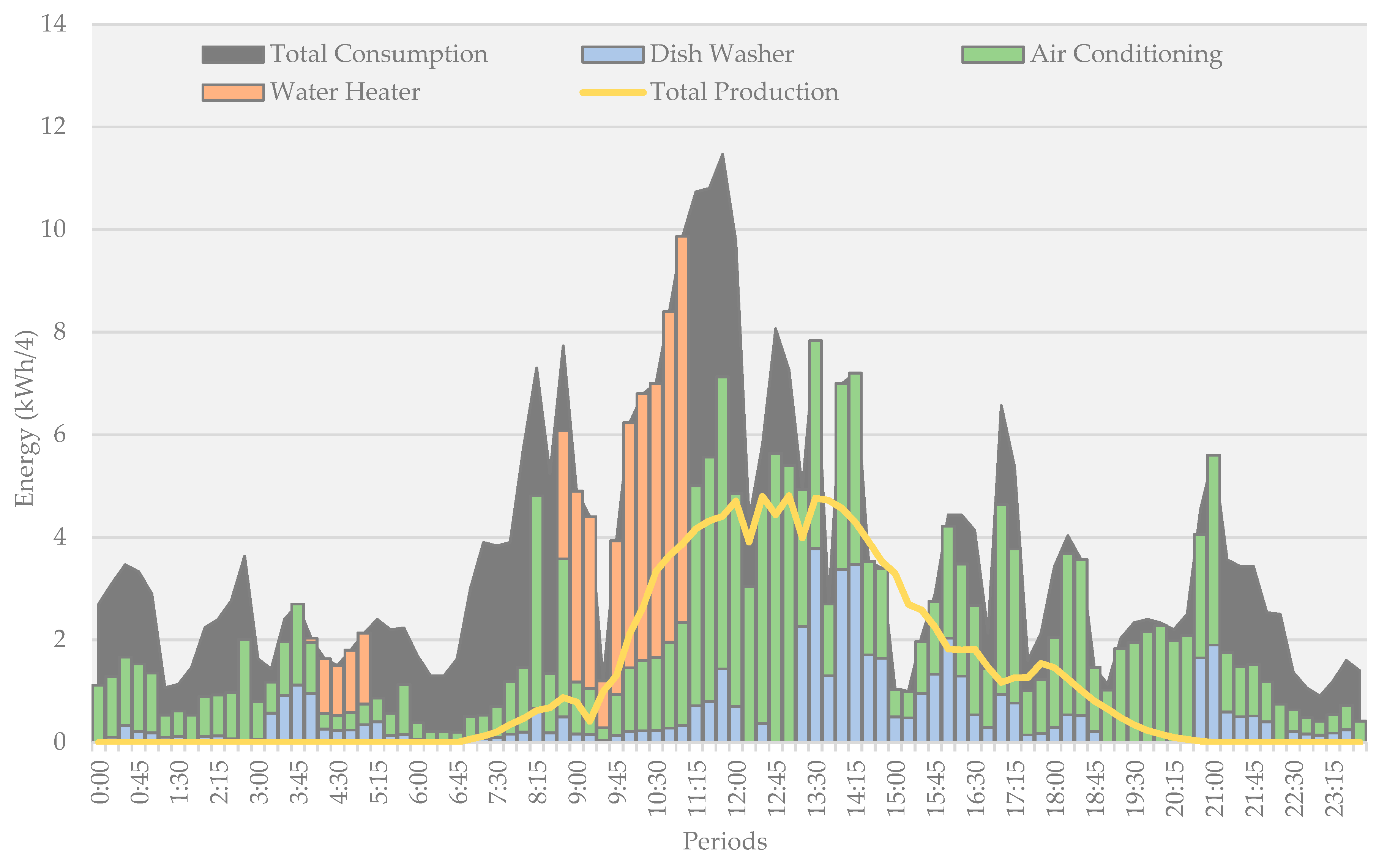
The system has two PV panels with different production, one has a maximum production of 7.5 kW and other has a maximum production of 2.5 kW. This PV panels and the battery storage unit are connected to the inverter. The battery can receive power from the PV production or the grid. In this case study, the inverter has two functionalities: the first is to convert the power from DC to AC and vice versa; the other functionality is to give the signal to manage certain loads. In this study, three different loads are considered: a dishwasher, an air conditioner, and a water heater. Figure 3 shows the disaggregated consumption and PV generation forecasts. In this case study, the forecast is performed for the next 24 h. In real-time operation, the forecast can be updated at every instant. Each time that user update the forecast can perform a new optimization. Regarding the influence of the forecasting results on optimization, in the case that the presented day-ahead forecasting strategies in References [30,31] are considered, the forecasting error, using Supporter Vector Machine algorithms to predict the values for the next 24 h, will be 9.11%.

Figure 3 presents a typical load profile with a peak of 11.5 kW at ~11.45 h. The consumption per controllable load is present in Figure 3 with different colors. The total consumption includes the sum of all loads and the same situation for PV but is the sum of two PV units. The peak of production is forecasted between the 12.00 h and 13.30 h with 6 kW. In some periods, such as 10:30, the sum of the controllable loads corresponds to the total consumption.

Table 3. Particle swarm optimization (PSO) parameters used.

Parameters	Symbol	Value
Population size	$j^{max}$	500
Maximum numbers of iterations	$i^{max}$	500
Maximum inertia weight	$w^{max}$	0.4
Minimum inertia weight	$w^{min}$	0.9
Maximum cognitive weight	$c_1^{max}$	1.5
Minimum cognitive weight	$c_1^{min}$	0.5
Maximum global weight	$c_2^{max}$	1.5
Minimum global weight	$c_2^{min}$	0.5
Number of evaluations	−	250,000
Number of trials	−	30

presents the parameters for PSO; they were obtained from a previous study.

The member of evaluation is equal to $j^{max}\times i^{max}$ and presents the number of fitness function is evaluated during the search process. Considering that the PSO is an algorithm of a random nature, a group of 30 trials is performed. With a sample of 30 results, it is possible to extract a more robust conclusion from the application of the PSO to the problem in question.

6. Results

This section presents the results and analysis obtained from the implementation of the proposed methodology and respective case study.

Table 4. Results for Equation (2) (€/day).

Resources Combination Scenarios		CPLEX	PSO
			Min	Mean	STD
Values optimized	PV + Bat + DR	3.1874	3.2771	3.3381	0.0469
	PV + Bat	7.8652	7.9454	8.0595	0.1169
	PV	8.8478	8.8478	8.8478	0
Nonoptimized values	PV + Bat	9.3298
	Without resources	16.8570

presents the results for Equation (1) in both the CPLEX (deterministic) obtaining the optimal value, and PSO obtained an approximate resolution. Four different scenarios were created considering the resources combination: the scenario “PV + Bat + DR” combine the all available resources (PV production, the storage capacity and loads flexibility), scenario “PV + Bat” combines the PV production and storage capacity resources and “PV” scenario only considers the PV production resource. The nonoptimized value is used as a base case scenario and was obtained by using a simple management mechanism; the scenario “PV + Bat” considers PV production and storage capacity, and the “Without resources” scenario does not consider any resource. Analyzing the results of CPLEX for the set of scenarios can conclude that “PV + Bat + DR” presents the smallest fitness function. It can be said with resources combinations brings benefits for household management.

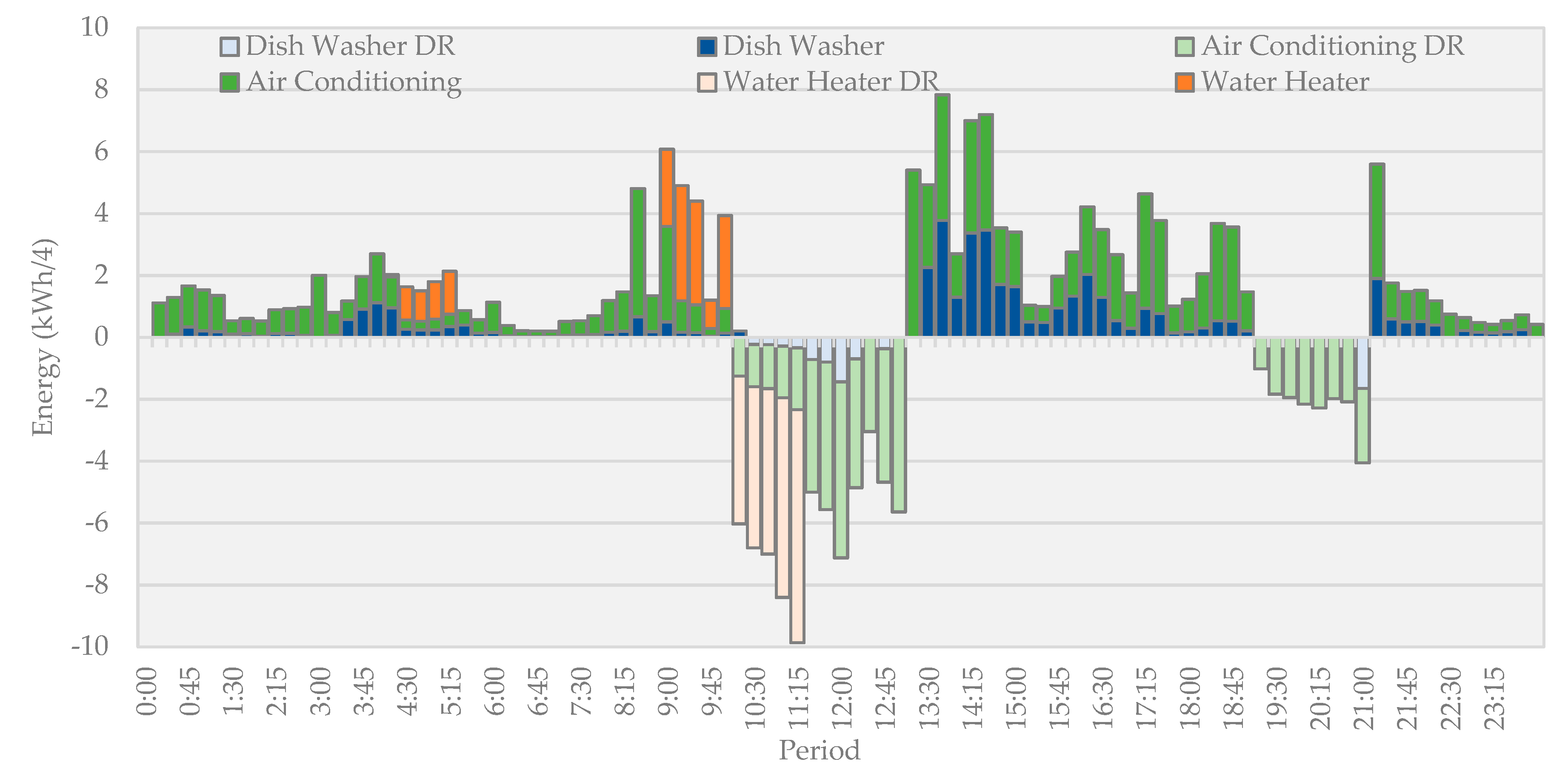
The analysis of results is performed for the “PV + Bat + DR” scenario. The results present in Table 4 of PSO correspond to 30 trials. The minimum value that the PSO reached is 2.8% higher when compared with CPLEX value. Analyzing the standard deviation (std) value for the sample of PSO results is possible to conclude that it is relatively small and the values of the 30 trials should be relatively close to the mean value. The STD analysis is important because it is a measure that expresses the degree of dispersion of 30 trials solutions. Figure 4 presented the results related to the DR actions applied to the profile shown in Figure 3.

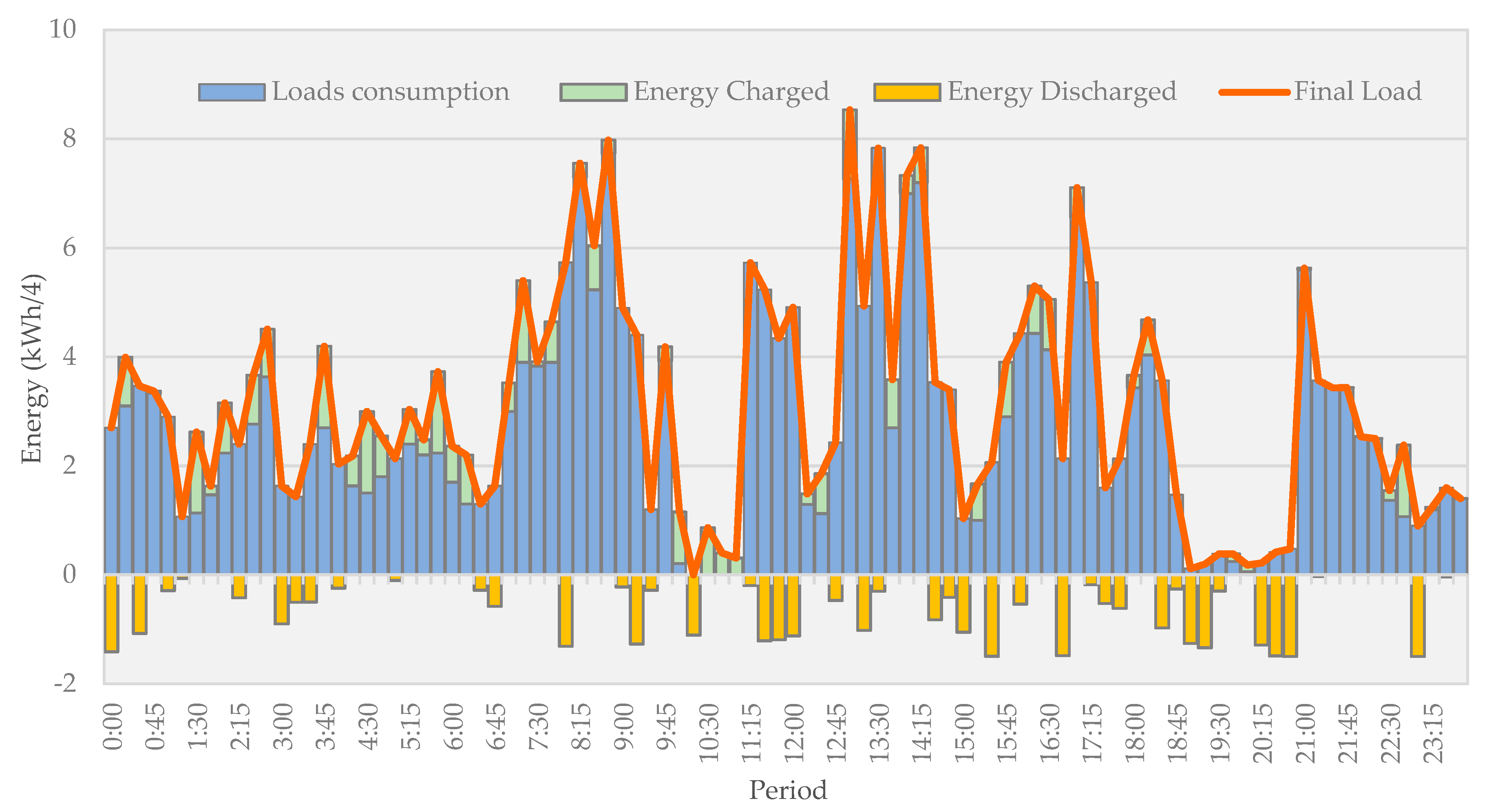
In Figure 4, the positive values correspond to the consumption of appliances that had no changes with the application of the methodology. Negative values are energy that has been reduced due to cut of loads. With the loads cut, reduction of 63% in the total consumption of three loads (dish washer, air conditioner, and water heater) was obtained. The DR actions are performed during 10.00 h to 13.00 h and 19.00 to 21.00. Crossing this information with Table 1, one can see that these periods correspond to a peak hour, precisely when energy is more expensive. During peak hours the consumption with the present optimization methodology is 44.8 kW, without its application and not considering PV generation and energy storage systems, the consumption will be 115.4 kW. This reduction represents 20% reduction of total daily consumption. In this way, it is concluded that the present methodology has an impact on the consumption of peak hours. In Figure 5 are presented the total load consumption (controllable and noncontrollable loads), the battery actions (charge and discharge), and the final load (load consumption plus battery charge).

Figure 5 shows that due to this condition, the generation (see Figure 3) exceeds the consumption needs, and in this case, the energy surplus will either be used to charge the battery or sell to the grid. In this way, the user avoids buying energy from the grid to charge the battery and to meet consumption necessities. The battery discharge cycles are mostly represented between 11.00 and 21.00 periods that correspond to a peak and intermediate hour.

Table 5. Summary of results.

Scenario	Method	Equation (1)	Equation (2)	Equation (3)	Daily Costs (€)	Daily Revenues (€)	Monthly Costs (€)
PV + Bat + DR	CPLEX	3.1874	3.1874	0	6.9380	3.7505	95.6233
PV + Bat + DR	PSO *	3.2771	3.2771	0	6.0565	2.7794	98.3140
PV + Bat	PSO *	7.9922	7.9922	0	8.5136	0.5683	239.7661
PV + Bat	Nonoptimized	9.3298	9.3298	0	9.3298	0	279.8928

* represent the values of trial with the minimum fitness value.

presents a summary of the results obtained by both methods applied.

With the proposed methodology, the daily cost of operation for CPLEX is 3.18 (€) and 3.28 (€) for PSO, but if the PV system, battery and DR do not exist and the daily costs are 16.83 (€). When compared the results of Table 5 is possible to observe that daily cost for CPLEX is larger compared to PSO daily cost, but the value of revenues in CPLEX are also large than PSO values. With the case study present in Section 5, the value of Equation (1) is equal to Equation (2) in both of methods, which means that the value of Equation (3) is zero because Equation (1) is the sum of Equation (2) and (3). When Equation (3) has the value zero represents that the DR is performed on periods with weight equal to zero and do not have a contribution to Equation (1). Table 5 also presents the monthly costs, which are calculated considering that the profile present in Figure 3 is repeated for the 30 days of the month. The value obtained for PSO is 2.96 (€) higher.

7. Conclusions

The present work addresses a methodology for resource scheduling (PV battery, storage capacity, and load flexibility) in a residential house that has not any contract with a DR service provider. Usually, the DR services for residential consumers are available using a DR service provider. In contrast, in the presented methodology the user is independent of applying his preferences in decision-making. In this case, the PV inverter, installed to convert the PV production into DC to AC, can control the charge or discharge of the battery system and the interruption of the loads. The optimization results for $P_{b,t}^{bat}$ and $P_{l,t}^{cut}$ are the inputs for the PV inverter control to act on the battery system and controllable loads.

The optimization problem was solved using a stochastic method (PSO) and a deterministic method (CPLEX). The results obtained by PSO have a close approximation to the deterministic results. The simple implementation and open access possibility of programming PSO over different platforms are factors that potentiate its use in this type of problems. In fact, in the present work, it was possible to demonstrate the results of running a PSO-based algorithm on a connection with the inverter of the PV system for control of the connected loads and the charge or discharge of the battery storage system.

The numerical results presented demonstrate that it is possible to obtain advantages by using the optimal combination of available resources. Table 4 presents the fitness function value for different resources combination, showing that the scenario that combines the all available resources is the best. Although PSO can obtain near-optimal solutions, its solution using the best combination resource scenario is better than the normal operating solution. With the comparison between the base scenario and the same scenario with PSO optimization, it is possible to make the assessment of the PSO approach. The daily cost optimized by PSO for the base scenario is 14% lower compared with the obtained in the nonoptimized base scenario.

As the presented methodology was built for been applied in an independent agent, the agent facility (residential house) needs to be prepared with equipment to perform the actions that the presented method imposes. This condition may be a weakness of the methodology, as it will increase the initial investment in equipment. Assuming that the DR program is implemented efficiently, such investment can be recovered over time, as the user does not need to pay fees to any service provider to use the service. The use of PSO instead of CPLEX can make the initial investment more appealing, for reasons already discussed in the introduction.

For future work, an analysis incorporating more DR actions (e.g., reduction and shifting capabilities) in the presented methodology can be done. Also, robust optimization considering the forecast error in PV production and domestic consumption can also be made to analyze the impact of forecasts errors in the electricity bill.

References

- European Union. The Strategic Energy Technology (SET) Plan; European Union: Brussels, Belgium, 2017. [Google Scholar]
- Parag, Y.; Sovacool, B.K. Electricity market design for the prosumer era. Nat. Energy 2016, 1, 16032. [Google Scholar] [CrossRef] [Green Version]
- Bhandari, B.; Lee, K.-T.; Lee, G.-Y.; Cho, Y.-M.; Ahn, S.-H. Optimization of hybrid renewable energy power systems: A review. Int. J. Precis. Eng. Manuf. Technol. 2015, 2, 99–112. [Google Scholar] [CrossRef] [Green Version]
- Roldán-Blay, C.; Escrivá-Escrivá, G.; Roldán-Porta, C. Improving the benefits of demand response participation in facilities with distributed energy resources. Energy 2019, 169, 710–718. [Google Scholar] [CrossRef]
- Paterakis, N.G.; Erdinç, O.; Catalão, J.P.S. An overview of Demand Response: Key-elements and international experience. Renew. Sustain. Energy Rev. 2017, 69, 871–891. [Google Scholar] [CrossRef]
- Neves, D.; Silva, C.A. Optimal electricity dispatch on isolated mini-grids using a demand response strategy for thermal storage backup with genetic algorithms. Energy 2015, 82, 436–445. [Google Scholar] [CrossRef]
- Jordehi, A.R. Optimisation of demand response in electric power systems, a review. Renew. Sustain. Energy Rev. 2019, 103, 308–319. [Google Scholar] [CrossRef]
- European Commission. Benchmarking Smart Metering Deployment in the EU-27 with a Focus on Electricity; European Commission: Brussels, Belgium, 2014. [Google Scholar]
- Nan, S.; Zhou, M.; Li, G. Optimal residential community demand response scheduling in smart grid. Appl. Energy 2018, 210, 1280–1289. [Google Scholar] [CrossRef]
- Zhang, D.; Shah, N.; Papageorgiou, L.G. Efficient energy consumption and operation management in a smart building with microgrid. Energy Convers. Manag. 2013, 74, 209–222. [Google Scholar] [CrossRef]
- Pina, A.; Silva, C.; Ferrão, P. The impact of demand side management strategies in the penetration of renewable electricity. Energy 2012, 41, 128–137. [Google Scholar] [CrossRef]
- Nwulu, N.I.; Xia, X. Optimal dispatch for a microgrid incorporating renewables and demand response. Renew. Energy 2017, 101, 16–28. [Google Scholar] [CrossRef]
- Alipour, M.; Zare, K.; Abapour, M. MINLP Probabilistic Scheduling Model for Demand Response Programs Integrated Energy Hubs. IEEE Trans. Ind. Inform. 2018, 14, 79–88. [Google Scholar] [CrossRef]
- Zhou, X.; Shi, J.; Tang, Y.; Li, Y.; Li, S.; Gong, K. Aggregate Control Strategy for Thermostatically Controlled Loads with Demand Response. Energies 2019, 12, 683. [Google Scholar] [CrossRef]
- Yao, Y.; Zhang, P.; Chen, S. Aggregating Large-Scale Generalized Energy Storages to Participate in the Energy and Regulation Market. Energies 2019, 12, 1024. [Google Scholar] [CrossRef]
- Spínola, J.; Faria, P.; Vale, Z. Photovoltaic inverter scheduler with the support of storage unit to minimize electricity bill. Adv. Intell. Syst. Comput. 2017, 619, 63–71. [Google Scholar]
- Hussain, B.; Khan, A.; Javaid, N.; Hasan, Q.; Malik, S.A.; Ahmad, O.; Dar, A.; Kazmi, A. A Weighted-Sum PSO Algorithm for HEMS: A New Approach for the Design and Diversified Performance Analysis. Electronics 2019, 8, 180. [Google Scholar] [CrossRef]
- Shen, J.; Jiang, C.; Li, B. Controllable Load Management Approaches in Smart Grids. Energies 2015, 8, 11187–11202. [Google Scholar] [CrossRef] [Green Version]
- Kong, D.-Y.; Bao, Y.-Q.; Hong, Y.-Y.; Wang, B.-B.; Huang, H.-B.; Liu, L.; Jiang, H.-H. Distributed Control Strategy for Smart Home Appliances Considering the Discrete Response Characteristics of the On/Off Loads. Appl. Sci. 2019, 9, 457. [Google Scholar] [CrossRef]
- Jordehi, A.R. A review on constraint handling strategies in particle swarm optimisation. Neural Comput. Appl. 2015, 26, 1265–1275. [Google Scholar] [CrossRef]
- Faria, P.; Vale, Z.; Soares, J.; Ferreira, J. Demand Response Management in Power Systems Using Particle Swarm Optimization. IEEE Intell. Syst. 2013, 28, 43–51. [Google Scholar] [CrossRef] [Green Version]
- Shehzad Hassan, M.A.; Chen, M.; Lin, H.; Ahmed, M.H.; Khan, M.Z.; Chughtai, G.R. Optimization Modeling for Dynamic Price Based Demand Response in Microgrids. J. Clean. Prod. 2019, 222, 231–241. [Google Scholar] [CrossRef]
- Aghajani, G.R.; Shayanfar, H.A.; Shayeghi, H. Demand side management in a smart micro-grid in the presence of renewable generation and demand response. Energy 2017, 126, 622–637. [Google Scholar] [CrossRef]
- Hu, M.; Xiao, F. Price-responsive model-based optimal demand response control of inverter air conditioners using genetic algorithm. Appl. Energy 2018, 219, 151–164. [Google Scholar] [CrossRef]
- Qian, L.P.; Wu, Y.; Zhang, Y.J.A.; Huang, J. Demand response management via real-time electricity price control in smart grids. Smart Grid Netw. Data Manag. Bus. Model. 2017, 169–192. [Google Scholar]
- Lezama, F.; Sucar, L.E.; de Cote, E.M.; Soares, J.; Vale, Z. Differential evolution strategies for large-scale energy resource management in smart grids. In Proceedings of the Genetic and Evolutionary Computation Conference Companion on GECCO ’17, Berlin, Germany, 15–19 July 2017; ACM Press: New York, New York, USA, 2017; pp. 1279–1286. [Google Scholar]
- Eberhart, R.; Kennedy, J. A new optimizer using particle swarm theory. In Proceedings of the Sixth International Symposium on Micro Machine and Human Science (MHS’95), Nagoya, Japan, 4–6 October 1995; pp. 39–43. [Google Scholar]
- Faia, R.; Pinto, T.; Vale, Z.; Corchado, J.M. Strategic Particle Swarm Inertia Selection for the Electricity Markets Participation Portfolio Optimization Problem. Appl. Artif. Intell. 2018, 32, 1–23. [Google Scholar] [CrossRef]
- ERSE Tarifas e Precos Para a Energia Eletrica e Outros Servicos em 2019. Available online: http://www.erse.pt/pt/electricidade/tarifaseprecos/2019/Documents/Diretiva ERSE 13-2018 (Tarifas e Preços EE 2019).pdf (accessed on 6 February 2019).
- Jozi, A.; Pinto, T.; Praca, I.; Vale, Z. Day-ahead forecasting approach for energy consumption of an office building using support vector machines. In Proceedings of the 2018 IEEE Symposium Series on Computational Intelligence (SSCI), Bangalore, India, 18–21 November 2018; pp. 1620–1625. [Google Scholar]
- Jozi, A.; Pinto, T.; Praça, I.; Vale, Z. Decision Support Application for Energy Consumption Forecasting. Appl. Sci. 2019, 9, 699. [Google Scholar] [CrossRef]
Figure 1.
Implementation scheme of the proposed work.
Figure 2.
The control scheme for the demand response (DR) cut with one load.
Figure 3.
Disaggregated consumption by appliance and photovoltaic (PV) generation.
Figure 4.
DR result regarding initial profile.
Figure 5.
Load consumptions, battery actions, and final load scheduling.