Dynamic Response of a Digital Displacement Motor Operating with Various Displacement Strategies

1
Department of Engineering and Science, University of Agder, 4879 Grimstad, Norway
2
Department of Energy Technology, Aalborg University, 9220 Aalborg East, Denmark
*
Author to whom correspondence should be addressed.
Energies 2019, 12(9), 1737; https://doi.org/10.3390/en12091737
Submission received: 31 March 2019
/
Revised: 25 April 2019
/
Accepted: 1 May 2019
/
Published: 8 May 2019
(This article belongs to the Special Issue Energy Efficiency and Controllability of Fluid Power Systems 2018)
Abstract
:Digital displacement technology has the potential of revolutionizing the performance of hydraulic piston pumps and motors. Instead of connecting each cylinder chamber to high and low pressure in conjunction with the shaft position, two electrically-controlled on/off valves are connected to each chamber. This allows for individual cylinder chamber control. Variable displacement can be achieved by using different displacement strategies, like for example the full stroke, partial stroke, or sequential partial stroke displacement strategy. Each displacement strategy has its transient and steady-state characteristics. This paper provides a detailed simulation analysis of the transient and steady-state response of a digital displacement motor running with various displacement strategies. The non-linear digital displacement motor model is verified by experimental work on a radial piston motor.
1. Introduction
Digital displacement machines are experiencing increased interest due to their high energy efficiency. Traditional variable displacement piston machines suffer from low energy efficiency when operating at partial displacements. They change displacement by changing the piston stroke. During one shaft revolution, every single cylinder chamber is pressurized, resulting in almost constant friction, leakage, and compressibility losses independent of displacement. In digital displacement machines, each cylinder chamber is connected to two electrically-operated on/off valves. By controlling the on/off valves, each cylinder chamber can be controlled individually. The chambers are only pressurized when necessary, resulting in losses that scale with the displacement, providing high energy efficiency even at partial displacements. A more detailed description of the digital displacement motor and pump technology can be found in [1,2,3,4].
Control of digital displacement machines is complicated and non-conventional. Due to the individual cylinder chamber control, it is hard to develop models that can be used for model-based design of feedback controllers. Both continuous, discrete, and hybrid dynamical system approximations have been investigated. The continuous and discrete approximations are sufficient to describe the fundamental dynamics if the number of cylinders and displacement fraction is sufficiently high [5,6,7,8,9,10,11]. In the case of applying linear control theory on a variable speed unit, the shaft speed of the machine should not be lower than the speed used during linearization of the system. The hybrid dynamic approximation has high accuracy, but is quite complex and, therefore not suitable for use in stability analyses and control design [12,13,14]. This is due to a large number of states and multiple jump maps and sets.
Since it is hard to develop models that can be used for control design purposes, it is highly relevant to know the dynamic behavior of digital displacement machines. Different displacement strategies give different transient and steady-state behavior in addition to different energy efficiency characteristics. The chosen displacement strategy should be decided based on operation requirements related to the driven application. Furthermore, one application may use different displacement strategies in different parts of the operation. The energy efficiency of different displacement strategies has been investigated in several papers [15,16,17], but the transient and steady-state characteristics have only been investigated in a limited number of papers. In Reference [18], the authors showed that the full stroke displacement strategy can achieve smooth system output if a proper cylinder chamber actuation sequence is used. A proper cylinder chamber actuation sequence is for example when every second chamber is actuated. The number of smooth output rates increases rapidly when the total number of pistons increases. In Reference [19], the authors compared the output ripples from full stroke to the output ripples from the partial stroke displacement strategy. The result showed that the full stroke displacement strategy has the lowest output ripples when the displacement is greater than 50%. When operating down at 20% displacement, the partial stroke displacement strategy had the lowest output ripples. At this time, the work done in [20] may be the most comprehensive description of the transient and steady-state characteristics of digital displacement machines. The work included both the full stroke, partial stroke, and sequential partial stroke displacement strategy. The results showed that the full stroke displacement strategy is most suited for high speed machines where energy efficiency is important. The partial stroke displacement strategy is most suited for low speed machines where both tracking performance and energy efficiency are important. The sequential partial stroke displacement strategy is most suited for very low-speed machines where control tracking performance is important and energy efficiency is of less importance. Still, a more detailed analysis of the dynamic behavior of digital displacement machines is missing.
This paper aims to compensate for the lack of knowledge regarding transient and steady-state characteristics for a digital displacement motor (DDM) operating with different displacement strategies. In all, three displacement strategies are analyzed: the full stroke displacement strategy (FSDS), the partial stroke displacement strategy (PSDS), and the sequential partial stroke displacement strategy (SPSDS). The analysis is conducted on a non-linear simulation model that is experimentally validated. The result shows that the transient response is highly affected by the shaft speed for some displacement strategies, but not for all. The steady-state response tends to oscillate due to switching between active and inactive cylinder chambers. The oscillations are affected by the chosen displacement strategy, the current displacement fraction, the number of pistons, and the shaft speed. The results of this analysis can be used to choose the most suitable displacement strategy when designing new controllers for DDMs.
The work presented in this paper is structured as follows: In Section 2, the non-linear DDM model is described. In Section 3, the analyzed displacement strategies are presented. The non-linear simulation model is validated in Section 4. In Section 5, the validated simulation model is used to analyze the transient and steady-state characteristics of the described displacement strategies. The results are then discussed in Section 6, and a conclusion is given in Section 7.
2. Simulation Model
This section describes the simulation model of the DDM. The simulated motor is a radial piston type with 15 pistons uniformly distributed around the shaft. The model was inspired by the model presented in [21]. A schematic representation of the DDM is shown to the right in Figure 1.
For simplicity, the governing equations are only derived for a single cylinder chamber, but the same method is used for all chambers. The governing equations are derived based on the single cylinder chamber shown to the left in Figure 1. It is assumed that each cylinder chamber is connected to a constant high and low pressure source and that friction and leakage are negligible. The main purpose of this study is to investigate the transient and steady-state response of the DDM. Neglecting the friction and leakage will not significantly influence the transient and steady-state response. Neglecting friction may result in a slightly higher magnitude of the output torque, but the main characteristics can still be analyzed.
The pressure dynamics in cylinder chamber i is calculated by using the continuity equation,
where is the effective bulk modulus of the hydraulic fluid, is the cylinder chamber volume, is the flow through the high pressure valve, and is the flow through the low pressure valve. The cylinder chamber volume, , and its time derivative are given by:
where is the dead volume in the cylinder chamber, is the piston displacement, is the local shaft position relative to the piston position, and is the shaft speed. The local shaft position is 0 rad when the piston is at top dead center (TDC). Due to the phase shift between the cylinders, the local shaft position, , is given by:
where is the shaft position and is the number of cylinders. The volume flow through the valves, and , is described by the orifice equation given by:
where and are the opening ratios of the high pressure valve and low pressure valve ranging from 0–1, where zero is fully closed and one is fully open. Both valves have the same flow-pressure coefficient, , and the same transient response. The transient response of the fast switching valves is described by a second-order system,
where and are the desired valve positions for the high pressure and low pressure valves, is the natural frequency of the valves, and is the damping ratio. The desired valve positions, and , are either zero or one and are given by the chosen valve actuation sequence. The valve actuation sequence is described in detail for each displacement strategy in Section 3.
The effective bulk modulus is calculated according to [22] as shown below:
where is the bulk modulus of the liquid and is the volume fraction of undissolved gas. The volume fraction of undissolved gas is calculated by:
where is the volume fraction of undissolved gas at atmospheric pressure, is the atmospheric pressure, and is the specific heat ratio.
The cylinder torque is given by:
and the DDM output torque is the sum of the torque contribution from all pistons:
Unless stated otherwise, the simulation parameters shown in Table 1 apply.
3. Displacement Strategies
The motor displacement can be changed by using different displacement strategies. This section describes the valve activation sequence for the displacement strategies analyzed in this paper. Note that only motor operation is described, but the same strategy can also be used for pumping operation.
3.1. Full Stroke Displacement Strategy
Full stroke is considered to be the simplest displacement strategy. The cylinder chambers are activated and deactivated for entire piston strokes. The fast switching on/off valves are only switched when the pistons are close to top dead center (TDC) or bottom dead center (BDC). In those piston positions, the valve flow is low, minimizing the valve throttling losses when switching the valves. Furthermore, the valves are timed only to be actuated when the pressure drop across them is small. The displacement of the motor is changed by changing the number of active cylinder chambers.
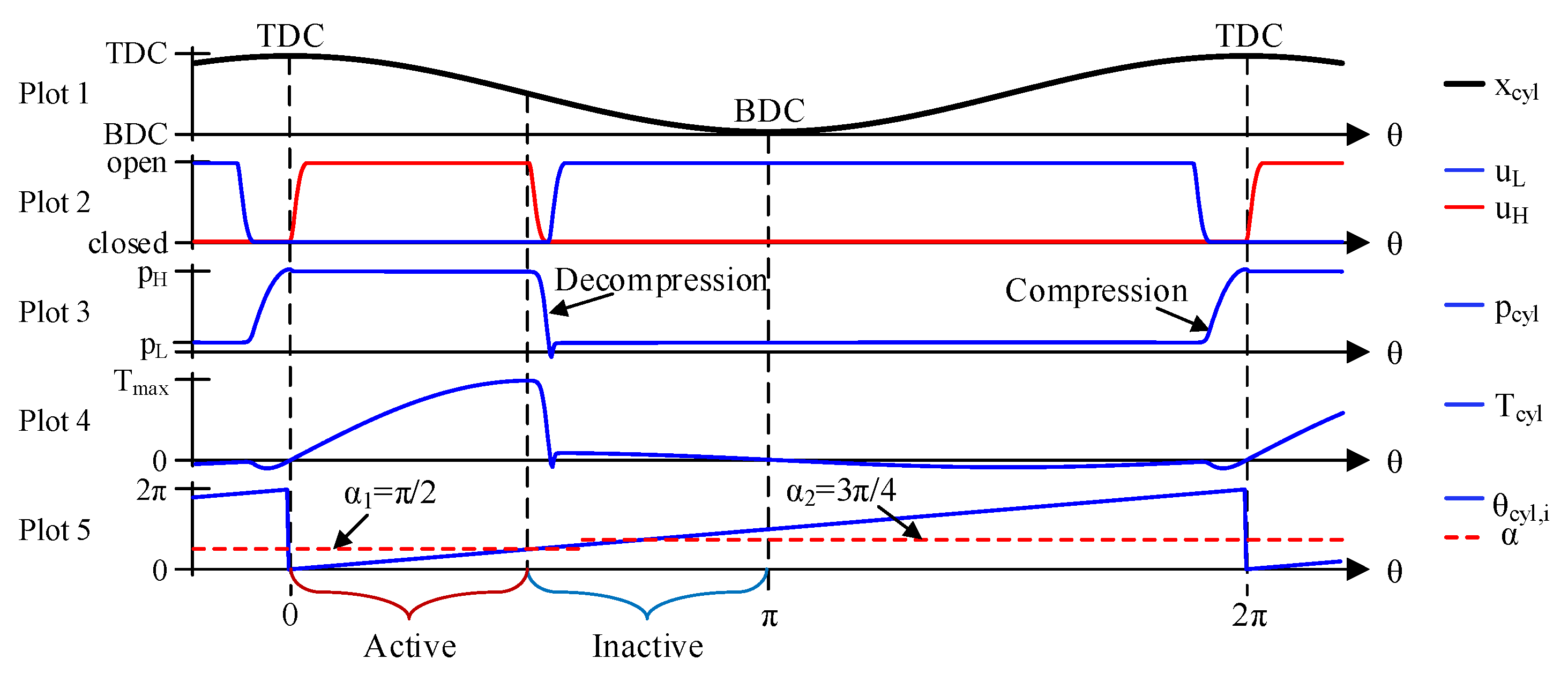
Figure 2 illustrates the valve timing strategy for a single cylinder chamber. Through the first shaft revolution, the chamber is deactivated, and through the second revolution, the chamber is activated. Plot 1 shows the piston position, Plot 2 the opening ratios of the valves, Plot 3 the chamber pressure, and Plot 4 the cylinder torque. For an inactive cylinder chamber, the high pressure valve is kept closed and the low pressure valve is kept open, resulting in only a very small torque contribution in the downstroke piston motion due to low chamber pressure. For an active cylinder chamber, the valves are switched close to TDC and BDC with the high pressure valve open during the downstroke piston motion and the low pressure valve open during the upstroke piston motion. The torque contribution is high due to the high chamber pressure in the downstroke motion. It can be seen that for the active cycle, the high pressure valve and low pressure valve are in the closed position at the same time. This is to compress and decompress the chamber oil in order only to switch the valves when the pressure drop across them is small, resulting in a minimum of flow peaks, pressure peaks, and valve throttling losses.
For each cylinder, the decision of activating or deactivating the cylinder chamber is taken at a fixed angle once every shaft revolution. This position is illustrated in Figure 2 with the decision angle . The desired displacement fraction, D, is a continuous signal ranging from 0–1, which corresponds to zero and full displacement, respectively. The displacement fraction is converted into a cylinder actuation sequence by a first-order delta-sigma modulator, which determines whether the current cylinder shall be active or inactive. This method was first proposed by Johansen et al. [23] and later used in several control papers [5,7,8,9]. A block diagram of the controller is shown in Figure 3.
Since the decision of activating or deactivating is made at a fixed shaft position ahead of TDC, the sampling time, , for the delta-sigma modulator is dependent on the number of cylinders and the rotational speed.
where is the shaft speed and is the number of cylinders. If the shaft speed is varying, the sampling time is also varying.
3.2. Partial Stroke Displacement Strategy
In PSDS, all cylinder chambers are activated during every shaft revolution, but only in a portion of the downstroke piston motion. The displacement of the motor is changed by increasing or decreasing the active part. In this study, two versions of PSDS were investigated. In Version 1, the cylinder chamber can only have one active period during the downstroke piston motion. In Version 2, the cylinder chamber can be reactivated and have more than one active period.
3.2.1. Version 1 of the Partial Stroke Displacement Strategy
Figure 4 shows the valve timing strategy for a single cylinder chamber operating with PSDS Version 1. The red dotted line in the bottom plot shows the state change angle . The state change angle, , describes at which local shaft position angle, , the cylinder shall change state from active to inactive. If , the cylinder is active, else the cylinder is inactive.
For the illustrated situation shown in Figure 4, the cylinder is active in the first half of the downstroke piston motion and deactivated in the remaining part, . This situation corresponds to 50% displacement. Increasing the state change angle after the cylinder has been deactivated will not result in a reactivation of the cylinder due to the nature of the PSDS Version 1. Once the cylinder is deactivated, it cannot be re-actuated before the next shaft revolution.
As for the FSDS, PSDS Version 1 also has a decompression phase and a compression phase in order only to switch the valves when the pressure difference across them is small, resulting in a minimum of pressure and flow peaks. Switching the valves mid-stroke will result in higher flow throttling losses during switching compared to switching the valves closer to TDC or BDC due to higher piston velocity and, therefore, higher valve flow. Hence, on/off valves used in PSDS should be faster compared to on/off valves used in FSDS to achieve the same energy efficiency at partial displacement [24].
The state change angle, , is calculated based on the desired displacement ratio, D. The desired displacement ratio is defined as the ratio between the intake volume during the active motoring period and the maximum intake volume [20]. Based on the calculation of the cylinder volume shown in Equation (2), the displacement ratio is calculated as shown below.
where is the intake volume during the active motoring period and is the maximum intake volume. The state changing angle, , is then calculated by rearranging Equation (14) as:
The state change angle, , is updated continuously until the state change is carried out. Figure 5 shows the block diagram of the open loop system. Note that due to the decompression phase shown in Figure 4, the displacement fraction needs to be less than 0.95 to use the last piston movement to decompress the cylinder.
3.2.2. Version 2 of the Partial Stroke Displacement Strategy
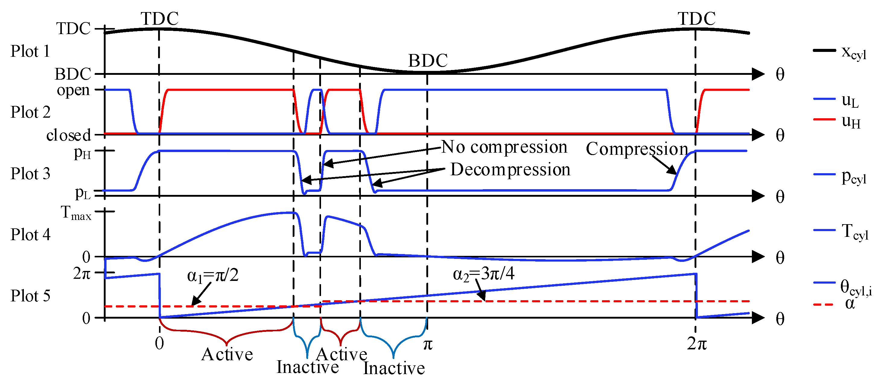
In PSDS Version 2, the cylinder is capable of being reactivated. Instead of only having one active period during the downstroke piston motion, the cylinder can be reactivated if the desired displacement ratio is changed; see Figure 6. First, the desired displacement ratio was set to , giving a state change angle of rad. When , the cylinder chamber changed state from active to inactive. After a small period, the desired displacement ratio was stepped up to which gave a state change angle of rad. Since , the cylinder was reactivated in the remaining rotation up to .
It is not possible to compress the cylinder oil before reactivating the cylinder due to downwards piston motion. The high pressure valve must therefore open against a high pressure difference. To avoid cavitation in the cylinder chamber, both the high and low pressure valves were actuated at the same time, opening the high pressure and closing the low pressure valve. Reactivation of a cylinder chamber may result in high flow throttling losses due to flow running directly from the high pressure source to the low pressure source until the low pressure valve is fully closed. An anti-cavitation valve can be included to avoid the risk of cavitation in the case of poor timing of the valves.
3.3. Sequential Partial Stroke Displacement Strategy
In SPSDS, one combination of active and inactive cylinders was used in a limited amount of time before a new cylinder combination was activated. The best cylinder combination can, for example, be found by an optimization algorithm or a search routine. This displacement strategy is characterized by frequent switchings and therefore lower efficiency compared to, for example, FSDS. In this section, only a short description of the SPSDS is given. A more detailed description can be found in [25].
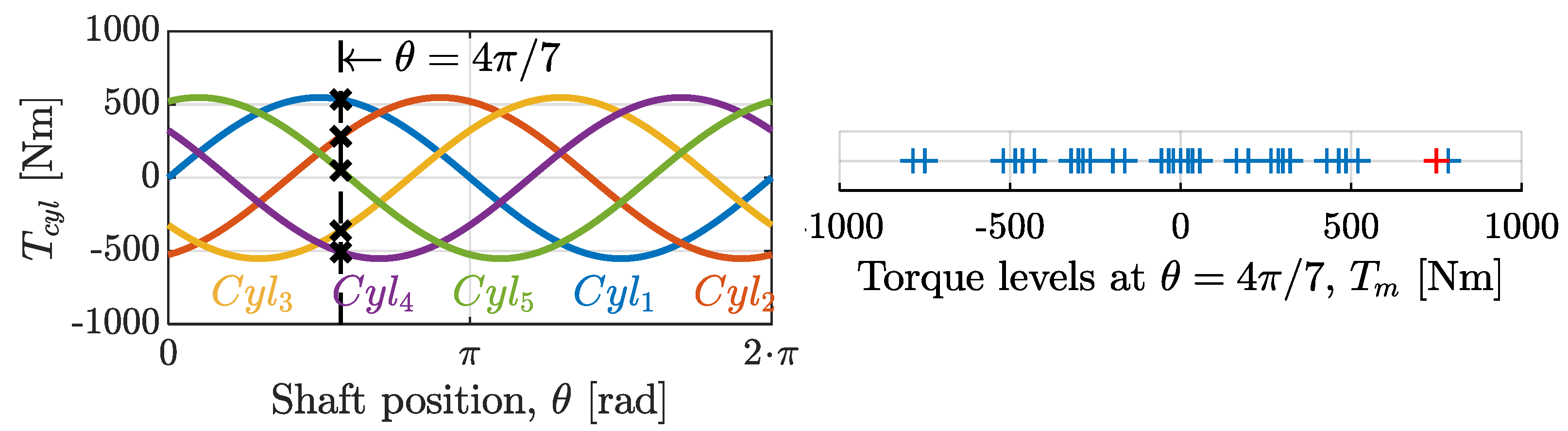
For simplicity, a five-cylinder motor will be used as an example when describing the concept of the SPSDS. For a five-cylinder motor, the cylinder states can be described by a 5-bit binary word, where “1” indicates that the cylinder is active and connected to the high pressure source and “0” indicates that the cylinder is inactive and connected to the low pressure source. The left plot in Figure 7 shows the cylinder torque contribution from a five-cylinder motor when all cylinders are activated for an entire shaft revolution. When rad, three chambers provided a positive torque, and two chambers provided a negative torque. For a five-piston motor, there are in all possible cylinder configurations. At rad, the 32 possible cylinder configurations gave only 31 distinct output torques because all cylinders connected to the high pressure source and all cylinders connected to the low pressure source gave the same output torque, Nm. The 31 distinct output torques when are shown in the right plot in Figure 7. The red point corresponds to activation of Cylinder Numbers 1 and 2 ().
Rotating the motor shaft one revolution with the same cylinder configuration will result in sinusoidal output torque. The cylinder configuration was therefore changed after a short period in order to meet the desired output torque. In this work, a search routine was used to find the best cylinder configuration. Figure 8 shows the block diagram of the controller. The input to the system was the desired motor torque, and the output was the actual motor torque. A search routine was used to find the best cylinder configuration based on the desired motor torque , the current motor shaft position , the motor shaft speed , and a look-up table. The look-up table was estimated offline and described the output torque , for all possible cylinder configurations at given shaft positions . In this work, the cylinder configuration, , was updated every ms and given by:
where k is the sample index and is the average output torque estimated from the look-up table over the interval of rotation to which the valve configuration, , will be applied. The applied interval is defined as where .
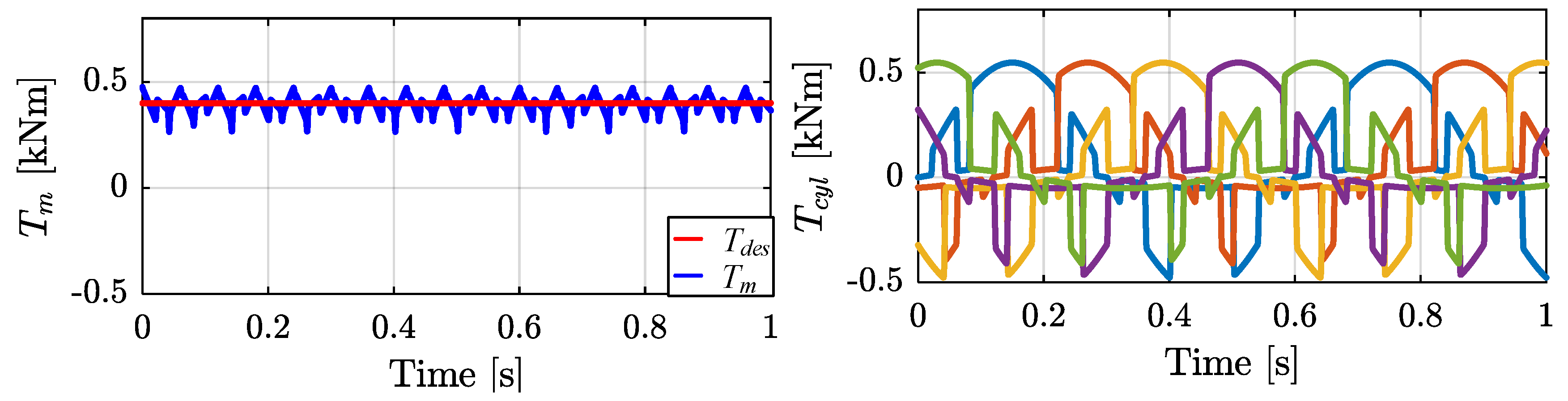
Figure 9 shows the result of the described controller for a five-cylinder motor. The red line in the left plot shows the desired motor torque, , and the blue line shows the actual motor torque, . The right plot shows the torque contribution from every single cylinder. It can be seen that the cylinder configuration was frequently switched and that the best cylinder configuration included both motoring and pumping cylinders.
4. Experimental Test Rig
In order to validate the simulation model of the DDM, a test rig has been developed. The test rig was designed to facilitate digital displacement operation on a single cylinder. It was assumed that all cylinders in the same motor had the same characteristics. Therefore, if the operation of one cylinder can be validated, the entire motor model is valid.
The test rig was based on a previously-developed test rig at Aalborg University, Denmark [24]. The previously-developed test rig was mainly developed to test the performance, durability, and power losses of novel prototype on/off valves used in digital displacement machine operation. The prototype valves were moving coil, moving magnet, and solenoid actuated poppet valves. Those poppet valves were designed to be passively opened. This limits the selection of displacement strategies. The test rig was therefore modified to operate with commercially-available valves that were able to open against high pressure difference in order to test the displacement strategies described in Section 3.
The following sections present the test rig, hydraulic diagram, and validation of the simulation model.
4.1. Test Rig Description
A test rig for testing different displacement strategies has been designed and built. The test rig is shown in Figure 10. The test rig was based on a five-cylinder Calzoni MR250 radial piston motor, which has been modified to operate with digital displacement technology on one cylinder. A permanent magnet synchronous electric machine was used to control the rotational speed. The control block was used to supply the modified radial piston motor with appropriate pressures and volume flows. The control block was supplied by a 250-kW variable displacement pump station, not shown in the picture. The power cabinet contained power supplies, valve drivers, a data acquisition system, and control systems.
4.1.1. Modification of the Hydraulic Motor
The hydraulic motor was modified to operate with digital displacement technology on a single cylinder. Figure 11 shows the modified hydraulic motor with the custom-made valve block. The valve block consisted of two on/off valves, two accumulators, three pressure sensors, and a pressure relief valve with anti-cavitation function. The on/off valves (1) and (2) were normally open WES-type valves from Bosch Rexroth. The flow capacity was approximately 45 L/min with a pressure drop of 5 bar. The switching time was below 5 ms. The hydraulic accumulators were 0.7-L diaphragm types from Bosch Rexroth. The low pressure accumulator (3) was pre-pressurized with 5 bar, and the high pressure accumulator (4) was pre-pressurized with 80 bar. There were in all three pressure transmitters mounted on the valve block. They measured the pressure in the low pressure source (5), high pressure source (6), and in the cylinder chamber (7). For safety reasons, a pressure relief valve with anti-cavitation function (8) was connected to the cylinder chamber to avoid very high cylinder chamber pressure and cavitation. A new top cover (10) for the modified cylinder has been designed and manufactured. This was done to block the original oil connection (12) between the port plate and the cylinder chamber and to create a new connection to the valve block. Also connected was an encoder on the motor shaft for shaft position measurements (not shown in Figure 11). Table 2 lists all parts used in the valve block.
4.1.2. Hydraulic Diagram
The hydraulic diagram for the test rig is shown in Figure 12. The hydraulic diagram was divided into three main parts; control block, valve block, and the non-modified cylinders. The control block delivered desired pressures and flows to the valve block and the non-modified cylinder chambers. The control block was designed to facilitate pumping, motoring, and idling (inactive) operation on the modified cylinder. In this study, only motor operation was used, and therefore, only motor operation will be described in this section. Pump operation was described in [26].
The pressure reducing valves (1, 3) were used to control the pressure in the high pressure line, , and in the intermediate pressure line, . The high pressure line was used to supply the modified cylinder chamber, and the intermediate pressure line was used to supply the four remaining cylinder chambers and for flushing of the machine casing by using the flow control valve (9). During motor operation, the 4/2 directional control valve (2) was set opposite of drawn, the gate valve (11) was open, the pressure relief valve (5) was set to high pressure level, and the remaining cylinder chambers were short circuited by setting the 3/2 directional control valve (7) opposite of drawn. The accumulators were used to reduce the pressure oscillations introduced by the digital displacement operation.
4.1.3. Sensors
In addition to measuring pressures, as shown in the hydraulic diagram in Figure 12, the shaft position and output torque were measured. An incremental Scancon encoder with 5000 ppr measured the shaft position, and an HBM T12 inductive torque transducer measured the output torque. The output torque was measured on the shaft connecting the radial piston motor to the permanent magnet synchronous electric machine.
4.2. Results from Experimental Work and Model Validation
The test rig has been used to validate the simulation model. The modified cylinder has been operated with FSDS, PSDS, and SPSDS. The experimental results have been compared to the simulation results. Table 3 shows the opening and closing angles used in both the experimental work and in the simulation model. Table 4 shows the operation conditions. The cylinder chamber dead volume in the simulation model has been increased from = 5.0 × 10⁻⁵ m3 (shown in Table 1) to = 1.308 × 10⁻⁴ m3 in order to use the same dead volume as in the experimental test setup.
4.2.1. Full Stroke Operation
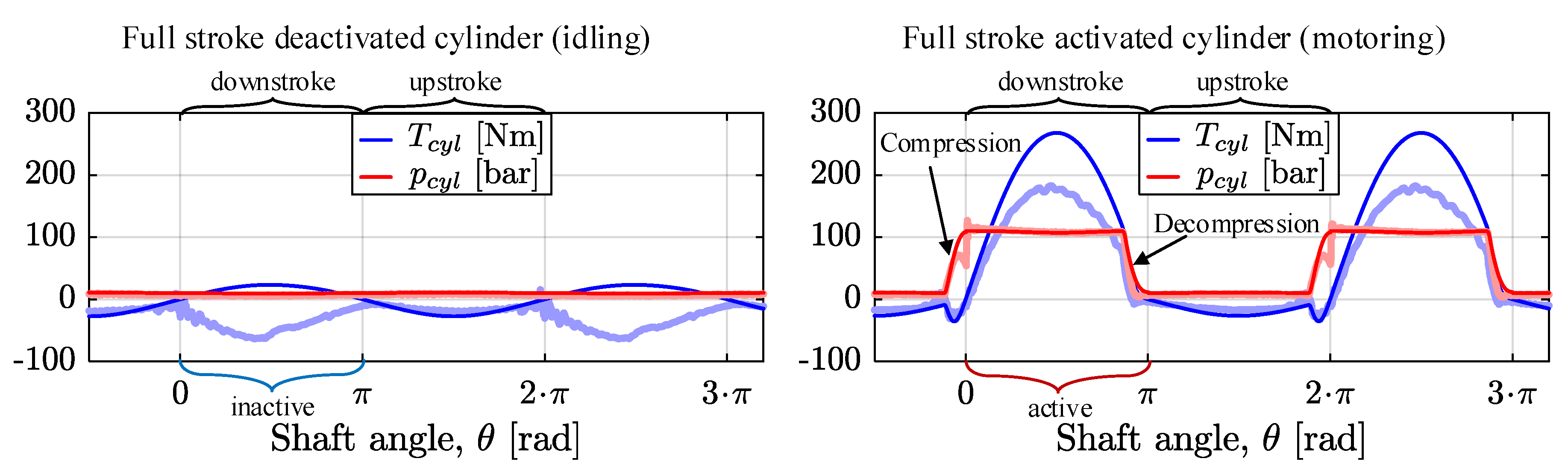
Figure 13 shows measured and simulated results of the cylinder pressure (red line) and cylinder torque (blue line) during full stroke operation as a function of the shaft position. Note that the cylinder was at TDC when rad and at BDC when rad. The left plot shows an inactive cylinder operation, and the right plot shows an active full stroke motor operation. The light colors show the experimental results, and the dark colors show the simulation results.
For the deactivated cylinder, the simulated chamber pressure matched the measured pressure. The simulated output torque matched the measured torque in the upstroke phase, but deviated in the downstroke phase. Some of the negative measured torque may be due to friction in the motor, but the non-modified cylinder chambers introduced most of it. As mentioned earlier, the four non-modified cylinder chambers were short circuited with a 1-L accumulator (15) connected to the short circuit line as shown in the hydraulic diagram in Figure 12. If all five cylinders had been short-circuited, the fluid volume in the short-circuited line would be relatively constant when rotating the radial piston motor. Since one cylinder was disconnected, the pressure in the non-modified cylinders would be higher in the downstroke phase than the upstroke phase. The black line in the left plot in Figure 14 shows the measured pressure in the short circuit line. The high pressure in the downstroke phase resulted in a negative torque contribution from the non-modified cylinders. This torque contribution was simulated by using the measured pressure. The green line, , shows the simulated torque from the non-modified cylinders added to the simulated cylinder torque, . By including the negative torque, the simulated and experimental measured torques had a close fit, seen by the green- and light blue-colored lines. The pre-charge pressure of the accumulator (15) was 20 bar. A pre-charge pressure of 20 bar was unnecessarily high and should have been reduced to reduce the torque contribution from the non-modified cylinders.
In the active full stroke motor cycle, shown to the right in Figure 13, the measured and simulated torque had the same trends. The simulated torque was a good match in the upstroke phase, but the measured torque had a lower magnitude in the downstroke phase due to the negative torque produced by the non-modified cylinders. The green line in the right plot in Figure 14 shows the simulated cylinder torque when the torque contribution from the non-modified cylinders was included, . The results show that the simulated and measured torques were a good match, seen by comparing the green- and light blue-colored lines. The simulated cylinder pressure matched the measured pressure quite well, except for small deviations in the compression and decompression phase, seen in the right plot in Figure 13. It can be seen that in the experimental work, the cylinder chamber fluid did not compress fully up to the high pressure level in the compression phase and decompressed slightly faster in the decompression phase. This may be due to leakage in the modified cylinder. In the simulation model, it was assumed that the cylinder was leak free. This assumption does not reflect reality. Some leakage was expected in order to reduce friction between moving parts in the cylinder. By including some leakage in the simulation model, the simulated pressure matched very well with the measured. The improvement can be seen in the compression and decompression phase in the right plot in Figure 14.
The leakage was included as shown in Equation (17).
where w is the width of the leakage path, h is the height of the leakage path, L is the length of the leakage path, is the viscosity of the hydraulic fluid, and is the drain pressure. The width of the leakage path was calculated as , where is the diameter of the cylinder chamber. The height of the leakage path was adjusted until the simulated pressure matched the measured pressure and kept within reasonable values. The drain pressure was set to bar.
4.2.2. Partial Stroke and Sequential Partial Stroke Operation
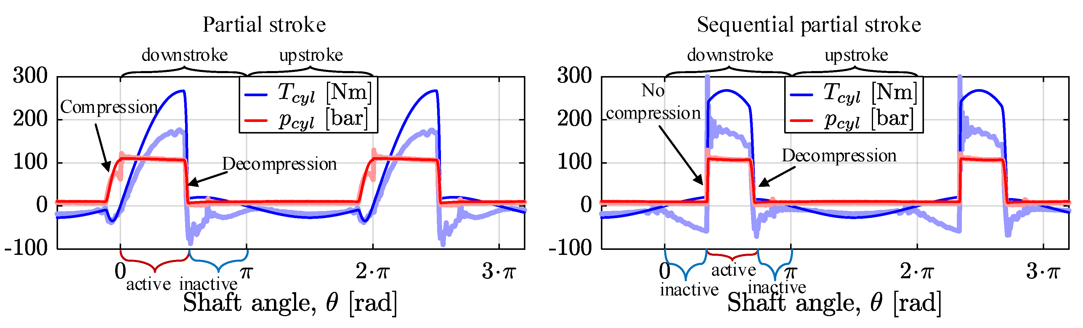
Figure 15 shows measured and simulated results of the chamber pressure (red line) and the cylinder torque (blue line) when motoring with PSDS Version 1 and SPSDS operation. In PSDS Version 1, shown to the left in Figure 15, the cylinder chamber was deactivated at rad. This corresponds to the most critical switching position due to maximum piston velocity. It can be seen that the measured and simulated chamber pressure matched quite well, except in the compression phase due to some leakage in the cylinder and some small oscillations right after rad and rad. In the downstroke phase, the measured and simulated cylinder torque had the same characteristics, but with a different magnitude due to the negative torque introduced by the non-modified cylinder chambers. In the upstroke phase, the measured and simulated output torque matched well.
In the sequential partial stroke operation sequence, shown to the right in Figure 15, there was no compression phase, because the cylinder chamber was activated during the downstroke piston motion. Hence, the cylinder volume was increasing, and the cylinder fluid can therefore not be compressed. The high pressure valve was opened at the same angle as the low pressure valve was closed. The measured and simulated pressure matched very well. The measured and simulated output torques matched very well in the upstroke phase, but deviated in the downstroke phase due to the negative torque introduced by the four non-modified cylinder chambers. However, the torque characteristics were the same, except for some small oscillations in the measured torque.
PSDS Version 1 was quite similar to PSDS Version 2, except that in Version 2, the cylinder can be reactivated. Reactivation of a cylinder was shown in SPSDS operation. The PSDS Version 2 was therefore considered as a combination of PSDS Version 1 and SPSDS. If the simulation model was valid for PSDS Version 1 and SPSDS, it was also assumed that it was valid for PSDS Version 2.
4.3. Discussion
In the experimental measurements, there was some insecurity due to sensor accuracy and alignment of shaft position and piston position. The piston position was not measured, but estimated based on the shaft position measurements. The piston position was an essential parameter considering proper activation of the on/off valves. The piston position was aligned with the shaft position measurements by comparing measured and simulated results of the output torque and cylinder pressure. A deviation in the range of a few degrees was therefore assumed.
There was also insecurity in the valve switchings. The valve position was not measured, and we can therefore not know exactly when the valves are switched. However, since we are operating at a low speed, approximately 100 rpm corresponding to 600 ms per revolution, a valve that opens a few milliseconds too late or too early will not significantly affect the result.
By comparing the measured and simulated results, it has been shown that the results matched quite well except for some deviation in the pressure due to leakage in the cylinder and some deviation in the torque due to negative torque introduced by the four non-modified cylinder chambers. The main purpose of this work was to analyze the output torque. By modifying all cylinders, it was assumed that the measured output torque would be closer to the simulated output torque. The deviation between measured and simulated pressure was great in the compression phase, but small in the decompression phase. Since the compression phase occurred close to TDC, an error in the chamber pressure would have very small influence on the total motor torque, because the torque contribution at this point was low. The simulation model was therefore assumed to be a valid model of the digital displacement motor.
5. Dynamic Response Analysis
This analysis describes the transient and steady-state characteristics for a DDM operating with different displacement strategies. This section is divided into three subsections. Each subsection covers the transient and steady-state analysis of one displacement strategy.
5.1. Full Stroke Displacement Strategy
In FSDS, the cylinders were enabled and disabled on a stroke-by-stroke basis. This subsection describes the transient and steady-state characteristics of the DDM operating with FSDS.
5.1.1. Transient Response for the Full Stroke Displacement Strategy
The decision of either activating or deactivating the cylinder chamber was made ahead of TDC, marked by in Figure 2. This decision would affect the output torque until the piston reached BDC. Hence, the motor shaft had to rotate more than a half revolution to change displacement fully. As a result, the response time was affected by the shaft speed. Therefore, this analysis started by analyzing the transient behavior in the shaft position domain.
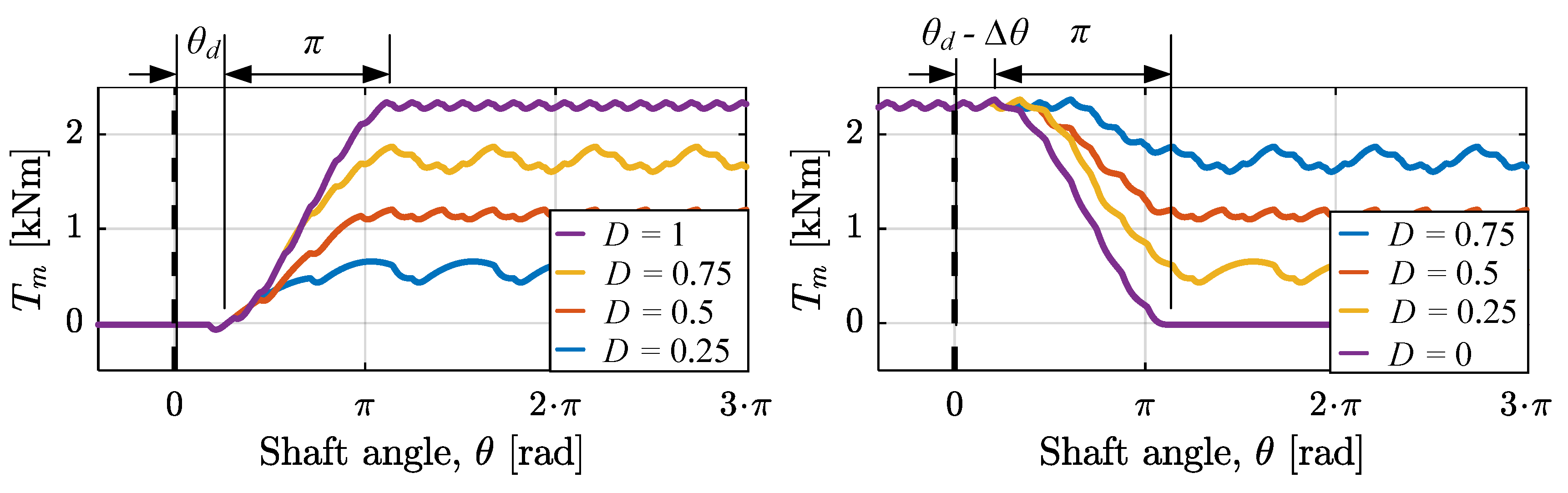
Figure 16 shows the step response in the shaft position domain. The left plot shows the step-up response when the displacement fraction, D, was stepped from zero up to 0.25, 0.5, 0.75, and 1. The right plot shows the step-down response when the displacement fraction, D, was stepped from one down to 0.75, 0.5, 0.25, and 0. The step was applied at rad. When stepping up, there was a small delay before the torque started to rise. This delay angle occurred since the decision of activating or deactivating the cylinder was made ahead of the compression phase. Right before the torque started to rise, there was a small drop in the torque due to the compression phase in the first activated cylinder. The response angle when stepping up was . The delay angle, , was calculated as: .
When stepping down, there is also a delay before reducing the motor torque. When stepping down to zero displacement, the delay occurred because the decision of activating or deactivating the cylinder was made ahead of the decompression phase, similar to the step-up case. The extended delay that occurred when stepping down to was due to the nature of the delta-sigma modulator. The response angle when stepping down was , where is the phase shift between the cylinders and given by .
Due to the nature of the delta-sigma modulator and the actuation sequence of previous cylinders, the step-up and step-down response angles were in some cases less than the maximum response angles, and . This phenomenon can be seen in Figure 17. For the simulated case, it can be seen that the response angle when stepping up deviated from the normal for the green and purple line. When stepping down, the step response angle deviated from the normal for the blue and red line.
In Figure 18, the step response is plotted in the time domain when stepping the displacement fraction from zero up to one at various speeds. It can clearly be seen that the response time was affected by the shaft speed. Assuming that the response angle was always at maximum, the response time was inversely proportional to the shaft speed.
5.1.2. Steady-State Response for the Full Stroke Displacement Strategy
The steady-state characteristics depend on the number of cylinders, the displacement fraction, and the shaft speed. Already in Figure 16, it can be seen that the steady-state torque tended to oscillate. This section will discuss how the number of cylinders, the shaft speed, and the displacement fraction affected the steady-state torque.
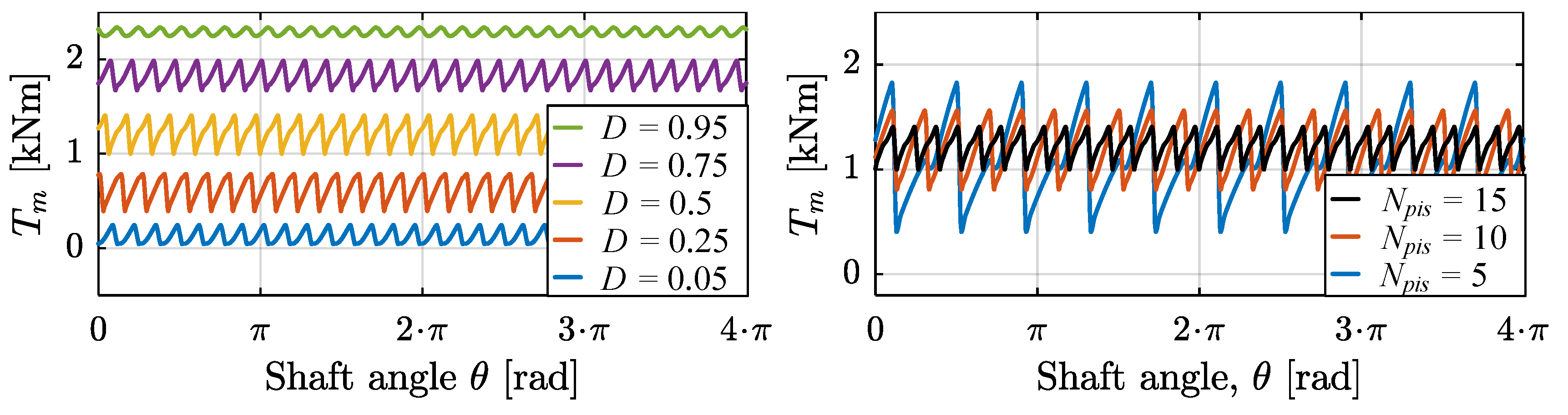
The left plot in Figure 19 shows the steady-state torque in the shaft position domain for motors with various numbers of cylinders and equal motor displacement. The right plot shows the steady-state torque from a 15-cylinder motor operating at various displacement fractions. From the left plot, it can be seen that the amplitude of the torque oscillations can be reduced by increasing the number of cylinders. From the right plot, it can be seen that for some selected displacements, for example , , and , the output torque was relatively smooth. On the other hand, only a small change in the displacement may change the cylinder actuation sequence and result in a significant torque peak or drop; see , , and . A significant torque peak or drop may not be very critical in high speed motors due to a very short duration, but more critical in very low speed motors where the exposure time is much longer. Off course, the inertia of the load will also affect the impact of a torque peak or drop. The number of smooth outputs can be increased by increasing the number of cylinders.
The frequency of the torque oscillations is affected by the rotational shaft speed. This can be seen in Figure 18 where the frequency of the steady-state oscillations was clearly increased when increasing the speed.
5.2. Partial Stroke Displacement Strategy
In PSDS, the cylinders were activated in only a portion of the downstroke piston motion. This section describes the transient and steady-state characteristics for both PSDS Version 1 and PSDS Version 2. Note that the steady-state characteristics were the same in Version 1 and Version 2.
5.2.1. Transient Response Version 1 of the Partial Stroke Displacement Strategy
In PSDS Version 1, the cylinders can only have one active period during the downstroke motion. Hence, the motor needs to rotate in order to increase displacement, similar to the FSDS. Therefore, the step response is constant in the shaft position domain, but will vary with shaft speed in the time domain. Figure 20 shows the step response in the shaft position domain. In the left plot, the displacement fraction was stepped up from 0.1 to 0.25, 0.5. 0.75, and 0.95. In the right plot, the displacement was stepped down from 0.95 to 0.75, 0.5, 0.25, and 0.1. The step was applied at rad.
From the left plot, it can be seen that there was no delay before increasing the torque, but the step-up response angle was affected by the magnitude of the applied step. A small step gave a small response angle. In fact, the relation between the change in the state change angle () and the response angle () was 1:1, or .
It can be seen that the step-down response angle was much lower than the step-up response angle. The step-down response angle was affected both by the response time of the valves and the angle the shaft needed to rotate in order to decompress the cylinders. Assuming that the valve was fast compared to the time it took for the shaft to rotate the distance needed to decompress the oil, the response angle was approximately equal to , where is the decompression angle.
Figure 21 shows the step response in the time domain at various speeds. The left plot shows the step-up response when the displacement ratio was stepped from 0.1–0.95. The right plot shows the step-down response when the displacement ratio was stepped down from 0.95–0.1. It can be seen that the step-down response time was much faster than the step-up response time. It can also bee seen that the response time was proportional to the speed. The step-up response time was equal to the time it took to rotate the step-up response angle (), and the step-down response time was equal to the time it took to rotate the step-down response angle ().
5.2.2. Transient Response Version 2 of the Partial Stroke Displacement Strategy
In PSDS Version 1, the step-up response time was much larger than the step-down response time. The step-up response time can be improved by using valves that can reactivate an already deactivated cylinder chamber. In PSDS Version 2, the step-up response time was constant and no longer affected by the motor speed, nor the magnitude of the step. This is shown in Figure 22. The left plot shows the step response in the time domain when stepping up at various speeds, and the right plot shows the step response in the time domain when stepping up to various displacement ratios with shaft speed kept constant. The left plot shows that the step-up response time was equal at various speeds. The step response was approximately equal to the response time of the on/off valves, which in this simulation was ms. The right plot shows that the response time was equal regardless of the magnitude of the displacement step, unlike PSDS Version 1.
5.2.3. Steady-State Response Partial Stroke Displacement Strategy
The steady-state response was characterized by small ripples and was equal for PSDS Version 1 and Version 2. The shape was constant in the shaft position domain, but the frequency would vary with the speed in the time domain. Therefore, the steady-state torque shape was analyzed in the position domain.
The amplitude of the ripples was affected by the used displacement ratio and the displacement of the cylinders. The left plot in Figure 23 shows the steady-state torque at different displacement ratios, and the right plot shows the steady-state torque for DDMs with various numbers of cylinders and equal motor displacement. The left plot shows that the maximum amplitude occurred when operating at 50% displacement. Fifty percent displacement corresponds to changing the cylinder state from active to inactive when . From Equation (11), it can be seen that at this shaft position, the torque contribution is at its highest. The smoothest output torque occurred when operating with very high or very low displacement ratios, meaning that the valves were switched close to TDC or BDC where the torque contribution from each cylinder was low. From the right plot, it can be seen that the amplitude was reduced when the number of cylinders was increased; meaning that the cylinder displacement was reduced and therefore also the torque contribution from each cylinder was reduced. The frequency of the ripples was also increased when the number of cylinders was increased. The shaft speed would also affect the frequency of the output torque ripples.
5.3. Sequential Partial Stroke Displacement Strategy
In SPSDS, the cylinders are activated for limited periods. The activation sequence was found by a search routine. In this section, the transient and steady-state characteristics of the SPSDS operation is analyzed.
5.3.1. Transient Response Sequential Partial Stroke Displacement Strategy
The step-up and step-down response in the time domain is shown in Figure 24. The step-up and step-down responses had no delay and were equal and independent of the magnitude of the step and the shaft speed. The response time was mostly affected by the response time of the on/off valves.
5.3.2. Steady-State Response Sequential Partial Stroke Displacement Strategy
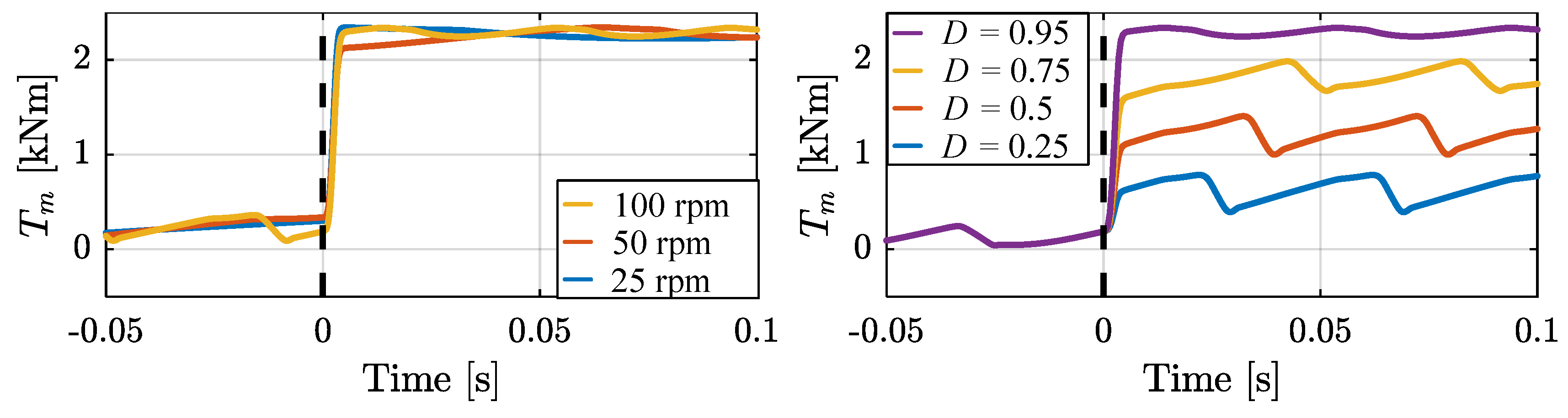
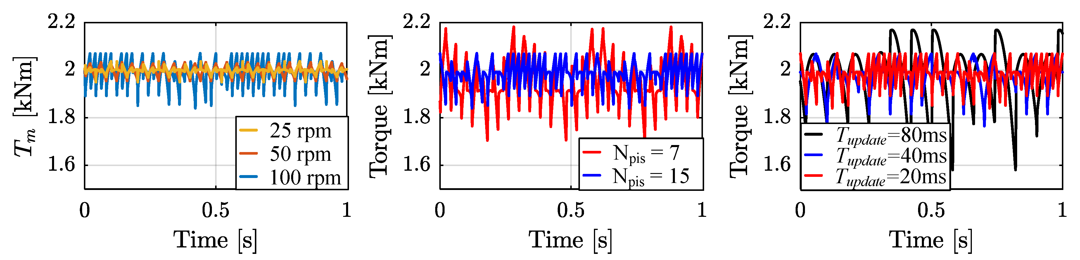
The steady-state torque tends to oscillate. The torque ripples are affected by the motor speed, the number of cylinders, and also the update frequency of the controller. In Figure 25, the desired torque was set to 2000 Nm. In the left plot, the motor was operated at various speeds, 100 rpm, 50 rpm, and 25 rpm, respectively. It can be seen that the torque ripples tended to decrease with shaft speed.
The middle plot shows the steady-state torque for two motors with equal motor displacement, but a different number of cylinders. The red line shows the output torque from a seven-piston motor, and the blue line shows the output torque from a 15-piston motor. It can be seen that the torque ripples were reduced when the number of cylinders was increased. This is because the number of possible cylinder configurations was affected by the number of cylinders (). By increasing the number of cylinders, the number of distinctive output levels would also be increased. Hence, the probability of finding a valve configuration that meets the desired output torque was increased.
The right plot in Figure 25 shows the motor output torque when the controller update frequency varied. The controller update time was set to 80 ms for the black line, 40 ms for the blue line, and 20 ms for the red line. A reduction in the torque ripples can be seen when the controller update time was changed from 80 ms and down to 40 ms. A further reduction in the torque ripples can be seen when the update time was decreased down to 20 ms.
The search routine used in this work is shown in Equation (16). Another search routine may also affect the torque ripples. It is not in the scope of this work to further investigate other search routines.
6. Discussion
In this section, the transient and steady-state response of the presented displacement strategies will be discussed. In Figure 26, both the input signal and the output torque are plotted when a sinusoidal input signal with increasing frequency is given. In order to be able to compare the output torque to the input signal, the values on the y-axis were normalized. The DDM was operating with FSDS in the first plot, PSDS Version 1 in the second plot, PSDS Version 2 in the third plot, and SPSDS in the last plot. The motor was operating at 50 rpm in all cases.
As shown earlier, the transient response when operating with FSDS is known to have a delay and is highly affected by the operation speed. This can clearly bee seen in the top plot. At low frequencies, the output torque was phase shifted to the input signal due to the delay. When increasing the frequency, the amplitude of the output torque started to decrease because of the high response time at low operation speeds. By increasing the operation speed, the time delay would be reduced and the amplitude would reach one for a higher input frequency. The FSDS is most suited for use in high speed operations due to the delay in the transient response and the fact that the response time is highly affected by the speed. The FSDS is also considered to be the most energy efficient displacement strategy due to few valve switchings and only actuating the valves close to TDC and BDC where the volume flow is low.
Both in FSDS and PSDS 1, the response time was highly affected by the operation speed. However, the response of PSDS Version 1 shown in the second plot in Figure 26 was much better than for FSDS, especially at low frequencies. This is because in PSDS Version 1, there was no delay, and the step up response time was affected by the magnitude of the step. A small step has a low response time. PSDS Version 1 is also known to have much faster response time when stepping down compared to stepping up. This is clearly seen when increasing the input frequency. The output torque followed the input signal in the torque reduction phase, but rose too slow in the torque increasing phase. The output torque tended to oscillate with small ripples. The magnitude of the ripples can be reduced by increasing the number of cylinders. The frequency was affected both by the number of cylinders and the operation speed. A small number of cylinders will result in a large magnitude of the ripples and should be avoided. Since the step-up response time is highly affected by the operation speed, this displacement strategy should only be used for medium and high speed operations. The controllability is considered to be higher than for FSDS, but the energy efficiency is considered to be lower due to activating all cylinder chambers and switching valves mid-stroke when the flow is high.
PSDS Version 2 can have more than one active period in one downstroke piston motion. This results in a response time that no longer is affected by the operation speed, but is closer to the response time of the on/off valves. The third plot in Figure 26 shows that the PSDS Version 2 had high controllability and followed the input signal very well, also at higher frequencies. The small torque ripples seen for the PSDS Version 1 can also be seen for the PSDS Version 2 (best seen at low frequencies). Due to reactivation of cylinder chambers, the energy efficiency will be lower than for PSDS Version 1 and FSDS. Because of the high controllability, also at low speeds, the PSDS Version 2 is most suited for low speed operations.
The SPSDS is characterized by frequently switchings. From the fourth plot in Figure 26, it can bee seen that the output torque followed the input signal very well. The output torque had some small ripples. Those ripples were smaller than for the PSDS, but will be increased if the speed increases, the number of cylinders is reduced, or the controller update frequency decreases. Due to the frequent switchings, the energy efficiency was the lowest of the investigated displacement strategies. SPSDS should only be used in very low speed operations because the torque ripples are increased at higher speeds.
The main characteristics of the investigated displacement strategies are summarized in Table 5.
7. Conclusions
In this paper, the transient and steady-state characteristics of a DDM operating with FSDS, PSDS Version 1, PSDS Version 2, and SPSDS have been investigated by simulations. The simulation model has been verified by experimental work.
The FSDS is characterized by a response time that is proportional to the velocity of the motor. Generally, the motor has to rotate approximately a half shaft revolution to change displacement fully. Due to the nature of the delta-sigma modulator, the response angle may vary in some cases. The output torque is relatively smooth, but for some displacements, a significant peak or drop in the output torque may occur. By increasing the number of cylinders, the number of smooth output torques will be increased. The FSDS struggles to follow a sinusoidal input signal when the motor speed is low. Therefore, if controllability is important, this displacement strategy should only be used in high speed units.
In this paper, two different versions of the partial stroke displacement strategy have been investigated. In Version 1, the cylinders can only have one active period during the downstroke piston motion. For this version, the motor had to rotate to increase the displacement. Therefore, the step-up response time was affected by the motor speed. The step-up response time was also affected by the magnitude of the step because the response angle was equal to the change of the state change angle, . The response time when stepping down was equal to the time it took to close the high pressure valve and decompress the deactivated cylinders, which was much faster than the response time when stepping up. The output torque tended to oscillate. The highest peaks occurred when operating at %, which corresponds to the switching state when the torque contribution from each cylinder is at its highest. The magnitude of the torque ripples will be reduced when operating with displacements closer to full or zero displacements. The magnitude can also be reduced by increasing the number of cylinders.
In PSDS Version 2, the step-up response time has been reduced by allowing the cylinders to be reactivated. Reactivating a cylinder will result in higher valve throttling losses and flow and pressure peaks in the system, but will also improve the controllability at low speeds. The step-up response time is no longer affected by the speed or the magnitude of the step, but by the response time of the on/off valves. When giving a sinusoidal input signal, the PSDS Version 1 struggles to increase the output torque fast enough at higher frequencies and should therefore only be used in medium and high speed operations. The PSDS Version 2 follows the input signal well even at high input frequencies and low speed. The controllability for Version 2 is, therefore, better than for PSDS Version 1 and is suitable for operation at low and medium speeds.
The SPSDS is characterized by frequent switching. The response time was approximately equal to the response time of the on/off valves. The output torque was smoother when operating at low speeds compared to high speeds. Increasing the number of cylinders will increase the number of possible output torques and thereby reduce the torque ripples. The SPSDS has high controllability and follows a sinusoidal input signal smoothly when operating at low speeds. SPSDS is suited for use in very low speed operations, but should be avoided in high speed operations due to increased torque, flow, and pressure ripples at higher speeds.
Author Contributions
Conceptualization, S.N.; methodology, S.N.; software, M.M.B.; validation, S.N. and M.M.B.; investigation, S.N.; writing, original draft preparation, S.N.; writing, review and editing, S.N., M.K.E., and T.O.A.
Funding
This research was funded by the Norwegian Research Council, SFIOffshore Mechatronics, Project Number 237896.
Conflicts of Interest
The authors declare no conflict of interest.
Abbreviations
| DDM | Digital displacement motor |
| FSDS | Full stroke displacement strategy |
| PSDS | Partial stroke displacement strategy |
| SPSDS | Sequential partial stroke displacement strategy |
| TDC | Top dead center |
| BDC | Bottom dead center |
References
- Rampen, W.H.S. The development of digital displacement technology. In Proceedings of the ASME/BATH Symposium in Fluid Power and Motion Control, Bath, UK, 15–17 September 2010. [Google Scholar]
- Ehsan, M.; Rampen, W.H.S.; Salter, S.H. Modeling of Digital-Displacement Pump-Motors and Their Application as Hydraulic Drives for Nonuniform Loads. J. Dyn. Syst. Meas. Control. 2000, 122, 210–215. [Google Scholar] [CrossRef]
- Payne, G.S.; Stein, U.B.; Ehsan, M.; Caldwell, N.J.; Rampen, W.H.S. Potential of digital displacement hydraulics for wave energy conversion. In Proceedings of the Sixth Europeam Wave and Tidal Energy Conference, Glasgow, UK, 29 August–2 September 2005; pp. 365–371. [Google Scholar]
- Rampen, W.H.S. Gearless Transmissions for Large Wind Turbines—The History and Future of Hydraulic Drives; Artemis IP Ltd.: Midlothian, UK, 2006. [Google Scholar]
- Pedersen, N.H.; Johansen, P.; Andersen, T.O. Feedback Control of Pulse-Density Modulated Digital Displacement Transmission using a Continuous Approximation. IEEE/ASME Trans. Mechatron. 2017. Status: Under 3rd revision. [Google Scholar]
- Johansen, P.; Roemer, D.B.; Andersen, T.O.; Pedersen, H.C. Discrete Linear Time Invariant of Digital Fluid Power Pump Flow Control. J. Dyn. Syst. Meas. Control 2017, 139, 101007. [Google Scholar] [CrossRef]
- Pedersen, N.H.; Johansen, P.; Andersen, T.O. Event-Driven Control of a Speed Varying Digital Displacement Machine. In Proceedings of the Bath/ASME Symposium on Fluid Power and Motion Control, Sarasota, FL, USA, 16–19 October 2017. [Google Scholar]
- Pedersen, N.H.; Johansen, P.; Andersen, T.O. LQR Feedback Control Development for Wind Turbines Featuring a Digital Fluid Power Transmission System. In Proceedings of the 9th Fluid Power Net International Ph.D. Symposium on Fluid Power, Florianópolis, Brazil, 26–28 October 2016. [Google Scholar]
- Pedersen, N.H.; Johansen, P.; Andersen, T.O. Optimal Control of a Wind Turbine with Digital Fluid Power Transmission. Nonlinear Dyn. 2018, 91, 591–607. [Google Scholar] [CrossRef]
- Pedersen, N.H.; Johansen, P.; Andersen, T.O. Model Predictive Control and Discrete Analysis of Partial Stroke Operated Digital Displacement Machine. In Proceedings of the IEEE Global Fluid Power Society PhD Symposium, Smara, Russia, 18–20 July 2018. [Google Scholar]
- Pedersen, N.H.; Johansen, P.; Hansen, A.H.; Andersen, T.O. Model Predictive Control of Low-Speed Partial Stroke Operated Digital Displacement Pump Unit. Model. Identif. Control 2018, 39, 167–177. [Google Scholar] [CrossRef]
- Pedersen, N.H.; Johansen, P.; Scheidl, R.; Andersen, T.O. Non-Linear Hybrid Control Oriented Modelling of a Digital Displacement Machine. In Proceedings of the 9th Workshop on Digital Fluid Power, Aalborg, Denmark, 7–8 September 2017. [Google Scholar]
- Pedersen, N.H.; Johansen, P.; Andersen, T.O. Four Qudrant Hybrid Control Oriented Dynamical System Model of Digital Displacement Units. In Proceedings of the Bath/ASME Symposium on Fluid Power and Motion Control, Bath, UK, 12–14 September 2018. [Google Scholar]
- Sniegucki, M.; Gottfried, M.; Klingauf, U. Optimal Control of Digital Hydraulic Drives using Mixed-Integer Quadratic Programming. In Proceedings of the 9th IFAC Symposium on Nonlinear Control Systems, Toulouse, France, 4–6 September 2013; pp. 827–832. [Google Scholar]
- Payne, G.S.; Kiprakis, A.E.; Ehsan, M.; Rampen, W.H.S.; Chick, J.P.; Wallace, A.R. Efficiency and dynamic performance of Digital Displacement™ hydraulic transmission in tidal current energy converters. Proc. Inst. Mech. Eng. Part A J. Power Energy 2007, 221, 207–218. [Google Scholar] [CrossRef]
- Merrill, K.J. Modeling and Analysis of Active Valve Control of Digtial PUMP-Motor. Ph.D. Thesis, Purdue University, West Lafayette, IN, USA, 2012. [Google Scholar]
- Heikkilä, M.; Tammisto, J.; Huova, M.; Huhtala, K.; Linjama, M. Experimental evaluation of a piston type digital pump-motor-transformer with two independent outlets. In Proceedings of the Bath/ASME Symposium on Fluid Power and Motion Control, Bath, UK, 15–17 September 2010. [Google Scholar]
- Linjama, M.; Huhtala, K. Digtal PUMP-Motor with Independent Outlets. In Proceedings of the 11th Scandinavian International Conference on Fluid Power, Linköping, Sweden, 2–4 June 2009. [Google Scholar]
- Merill, K.J.; Lumkes, J.H., Jr. Operating Strategies and Valve Requirements for Digtal PUMP/Motors. In Proceedings of the 6th FPNI-Phd Symposium, West Lafayette, IN, USA, 15–19 June 2010. [Google Scholar]
- Pedersen, N.H.; Johansen, P.; Hansen, A.H.; Andersen, T.O. Challenges with Respect to Control of Digital Displacement Hydraulic Units. Model. Identif. Control 2018, 39, 91–150. [Google Scholar] [CrossRef]
- Roemer, D.B. Design and Optimization of Fast Switching Valves for Large Scale Digital Hydraulics Motors. Ph.D. Thesis, Aalborg University, Aalborg, Denmark, 2014. [Google Scholar]
- Hansen, M.R. Fluid stiffness. In Compendium Fluid Mechanics; Lecture notes MAS126; Department of Engineering, University of Agder: Grimstad, Norway, 2015; pp. 28–30. [Google Scholar]
- Johansen, P.; Roemer, D.B.; Andersen, T.O.; Pedersen, H.C. Delta-Sigma Modulated Displacement of a Digital Fluid Power Pump. In Proceedings of the Seventh Workshop on Digital Fluid Power, Linz, Austria, 26–27 February 2015. [Google Scholar]
- Nørgård, C. Design, Optimization and Testing of Valves for Digital Displacement Machines. Ph.D. Thesis, Aalborg University, Aalborg, Denmark, 17 October 2017. [Google Scholar]
- Armstrong, B.S.; Yuan, Q. Multi-Level Control of Hydraulic Gerotor Motors and Pumps. In Proceedings of the American Control Conference, Minneapolis, MN, USA, 14–16 June 2006; pp. 4619–4626. [Google Scholar]
- Nørgård, C.; Christensen, J.H.; Bech, M.M.; Hansen, A.H.; Andersen, T.O. Test rig for valves of digital displacement machines. In Proceedings of the 9th Workshop on Digital Fluid Power, Aalborg, Denmark, 7–8 September 2017. [Google Scholar]
Figure 1.
Sketch of a single cylinder chamber (left) and a 15-piston DDM (right).

Figure 2.
Valve timing schematics for the full stroke displacement strategy.

Figure 3.
Schematic of the open loop control system for FSDS.

Figure 4.
Valve timing schematics for partial stroke displacement strategy Version 1.

Figure 5.
Schematic of open loop control for PSDS (equal for Version 1 and Version 2).

Figure 6.
Valve timing schematics for partial stroke displacement strategy Version 2.

Figure 7.
Cylinder torque (left plot) and possible torque levels at (right plot).

Figure 8.
Schematic of open loop control for SPSDS.

Figure 9.
Example of DDM operation with SPSDS.

Figure 10.
Test rig.

Figure 11.
Illustration of the modified radial piston motor.

Figure 12.
Hydraulic diagram of the test rig [26].
Figure 12.
Hydraulic diagram of the test rig [26].

Figure 13.
Experimental and simulation results for idling and full stroke motor operation (light color is experimental results, and dark color is simulation results).
Figure 13.
Experimental and simulation results for idling and full stroke motor operation (light color is experimental results, and dark color is simulation results).

Figure 14.
Experimental and simulated results for full stroke motor operation when leakage was introduced in the simulation model (light color is experimental results, and dark color is simulation results).
Figure 14.
Experimental and simulated results for full stroke motor operation when leakage was introduced in the simulation model (light color is experimental results, and dark color is simulation results).

Figure 15.
Experimental and simulated results for partial stroke and sequential partial stroke motor operation (light color is experimental results, and dark color is simulation results).
Figure 15.
Experimental and simulated results for partial stroke and sequential partial stroke motor operation (light color is experimental results, and dark color is simulation results).

Figure 16.
Step-up response (left plot) and step-down response (right plot) using FSDS in the position domain.
Figure 16.
Step-up response (left plot) and step-down response (right plot) using FSDS in the position domain.

Figure 17.
Step-up response (left plot) and step-down response (right plot) using FSDS with variable response angles.
Figure 17.
Step-up response (left plot) and step-down response (right plot) using FSDS with variable response angles.

Figure 18.
Transient response FSDS in the time domain operating at various speeds.

Figure 19.
Steady-state response FSDS with various numbers of cylinders (left plot) and at various displacements (right plot).
Figure 19.
Steady-state response FSDS with various numbers of cylinders (left plot) and at various displacements (right plot).

Figure 20.
Step-up response (left plot) and step-down response (right plot) using PSDS Version 1 in the position domain.
Figure 20.
Step-up response (left plot) and step-down response (right plot) using PSDS Version 1 in the position domain.

Figure 21.
Step-up response (left plot) and step-down response (right plot) using PSDS Version 1 in the time domain operating at various speeds.
Figure 21.
Step-up response (left plot) and step-down response (right plot) using PSDS Version 1 in the time domain operating at various speeds.

Figure 22.
Transient response PSDS Version 2 in the time domain at various speeds (left plot) and displacement step up to various displacements (right plot).
Figure 22.
Transient response PSDS Version 2 in the time domain at various speeds (left plot) and displacement step up to various displacements (right plot).

Figure 23.
Steady-state response PSDS at various displacements (left plot) and with various numbers of cylinders (right plot).
Figure 23.
Steady-state response PSDS at various displacements (left plot) and with various numbers of cylinders (right plot).

Figure 24.
Step-up response (left plot) and step-down response (right plot) using SPSDS in the time domain.
Figure 24.
Step-up response (left plot) and step-down response (right plot) using SPSDS in the time domain.

Figure 25.
Steady-state response SPSDS at various shaft speeds (left plot), with various numbers of cylinders (mid plot) and various controller update frequencies (right plot).
Figure 25.
Steady-state response SPSDS at various shaft speeds (left plot), with various numbers of cylinders (mid plot) and various controller update frequencies (right plot).

Figure 26.
DDM torque response with a sinusoidal input signal operating at 50 rpm.


Table 1.
Simulation parameters.
| Parameter | Symbol | Value | Unit |
|---|---|---|---|
| Piston chamber displacement | 50 | cc/rev | |
| Cylinder chamber dead volume | 50 | cc | |
| Number of pistons | 15 | − | |
| Motor speed | 100 | rpm | |
| Switching time on/off valves | 5 | ms | |
| Flow-pressure coefficient | 1.2 × 10⁶ | ·s/m3 | |
| High pressure | 220 | bar | |
| Low pressure | 20 | bar | |
| Bulk modulus liquid | 1.2 | GPa | |
| Volume fraction of undissolved gas at | 0.01 | − |
Table 2.
Part list of the modified motor.
| Description | Part Number | Ordering Code | Manufacturer |
|---|---|---|---|
| On/off valve | 1 and 2 | 3WES 8 P1XK/AG24CK50/V | Bosch Rexroth |
| Accumulator | 3 and 4 | HAD-0.7-250-1x/50Z06A-1N111-BA | Bosch Rexroth |
| Pressure transducer | 5 | HM 20-2x-100-H-K35 | Bosch Rexroth |
| Pressure transducer | 6 and 7 | HM 20-2x-400-H-K35 | Bosch Rexroth |
| Pressure relief valve | 8 | PLC053 393000K179 | Parker |
| Hydraulic motor | 16 | MR250D-P1Q1N1C1N07 00 | Delivered by Parker |
| Position encoder | - | SCH32F-5000-D-08-26-65-00-S-C8-S3 | Scancon |
Table 3.
Activation angles.
| FSDS | PSDS | SPSDS | |
|---|---|---|---|
| Open HPV | 0° | 0° | 60° |
| Close HPV | 154° | 90° | 120° |
| Open LPV | 180° | 94° | 125° |
| Close LPV | 338° | 338° | 60° |
Table 4.
Operation conditions.
| Description | Symbol | Value |
|---|---|---|
| Operation speed | 100 rpm | |
| High pressure level | 110 bar | |
| Low pressure level | 10 bar |
Table 5.
Summary of transient and steady-state characteristics.
| FSDS | PSDS Version 1 | PSDS Version 2 | SPSDS | ||
|---|---|---|---|---|---|
| Transient response | Delay-time | Some delay due to decision angle ahead of TDC | No delay | No delay | No delay |
| Response time | Affected by shaft speed | Affected by shaft speed and displacement step | Affected by valve response time | Affected by valve response time | |
| Overshoot | No overshoot | No overshoot | No overshoot | No overshoot | |
| Steady-state response | Magnitude of torque ripples | Affected by displacement ratio and number of cylinders | Affected by displacement ratio and number of cylinders | Affected by displacement ratio and number of cylinders | Affected by shaft speed, controller update rate & number of cylinders |
| Frequency of torque ripples | Affected by shaft speed and number of cylinders | Affected by shaft speed and number of cylinders | Affected by shaft speed and number of cylinders | Affected by controller update rate |
© 2019 by the authors. Licensee MDPI, Basel, Switzerland. This article is an open access article distributed under the terms and conditions of the Creative Commons Attribution (CC BY) license (http://creativecommons.org/licenses/by/4.0/).
Share and Cite
MDPI and ACS Style
Nordås, S.; Beck, M.M.; Ebbesen, M.K.; Andersen, T.O. Dynamic Response of a Digital Displacement Motor Operating with Various Displacement Strategies. Energies 2019, 12, 1737. https://doi.org/10.3390/en12091737
AMA Style
Nordås S, Beck MM, Ebbesen MK, Andersen TO. Dynamic Response of a Digital Displacement Motor Operating with Various Displacement Strategies. Energies. 2019; 12(9):1737. https://doi.org/10.3390/en12091737
Chicago/Turabian StyleNordås, Sondre, Michael M. Beck, Morten K. Ebbesen, and Torben O. Andersen. 2019. "Dynamic Response of a Digital Displacement Motor Operating with Various Displacement Strategies" Energies 12, no. 9: 1737. https://doi.org/10.3390/en12091737
Note that from the first issue of 2016, this journal uses article numbers instead of page numbers. See further details here.