A Class of Energy Efficient Self-Contained Electro-Hydraulic Drives with Self-Locking Capability


1
Department of Energy Technology, Aalborg University, Pontoppidanstraede 111, 9220 Aalborg, Denmark
2
Bosch Rexroth A/S, Gungevej 1, 2650 Hvidovre, Denmark
*
Author to whom correspondence should be addressed.
Energies 2019, 12(10), 1866; https://doi.org/10.3390/en12101866
Submission received: 29 March 2019
/
Revised: 24 April 2019
/
Accepted: 10 May 2019
/
Published: 16 May 2019
(This article belongs to the Special Issue Energy Efficiency and Controllability of Fluid Power Systems 2018)
Abstract
:Pump controlled and self-contained electro-hydraulic cylinder drives may improve energy efficiency and reduce installation space compared to conventional valve solutions, while being in line with the trend of electrification. The topic has gained increasing interest in industry as well as in academia in recent years. However, this technology has failed to break through in industry on a broad scale, with the reason assumed to be lack of meeting industry requirements. These requirements include high drive stiffness enabling a large application range, and the ability to maintain cooling and filtration in required ranges, enabling proper reliability and durability. Furthermore, at this point the cost of realization of such drives is comparable only to high end valve drive solutions, while not providing dynamics on a similar level. An initiative to improve this technology in terms of a class of drives evolving around a hydraulic cylinder locking mechanism is proposed. The resulting class of drives generally rely on separate cylinder forward and return flow paths, allowing for fluid cooling and filtration as well as control of the drive stiffness. The proposed class of drives is analyzed regarding energy loss and recovery potential, a basic model based control design is realized, and the industrial feasibility of the drive class is considered. It is found that the proposed class of drives may be realized with standard components maintained in their design ranges at competitive costs compared to conventional valve solutions. Furthermore, it is found that pressure levels may be controlled in a proper way, allowing to produce either highly efficient operation or a high drive stiffness.
1. Introduction
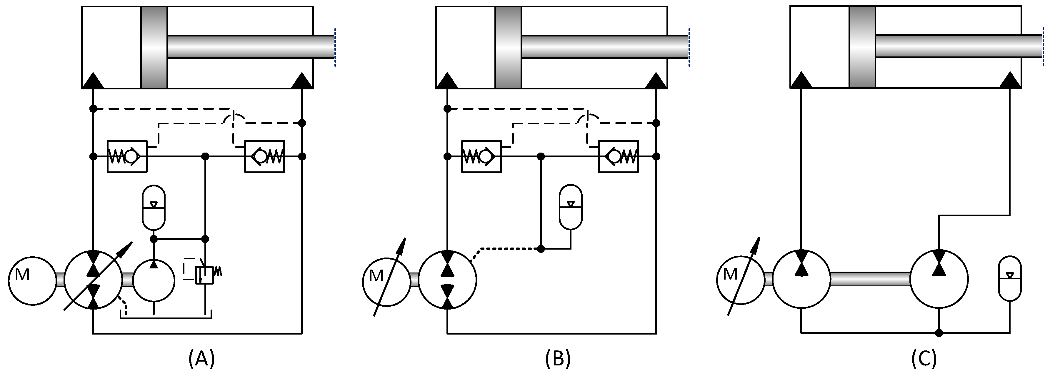
In recent years pump operated hydraulic drives for differential cylinder actuation have gained increasing interest, both in academia and in the industry. Naturally, it is intriguing to control cylinders without the main flows realized via throttle control and thereby avoid the associated losses. Such drives have been considered with both conventional reservoirs and fully self-contained drives, using either variable displacement- or speed-variable (fixed displacement) pumps. Various architectures with one or more pumps have been investigated, with the drive architectures in Figure 1 being the more predominant in literature. An overview of the works conducted in relation to these are given in the following discussion, and a thorough review on the topic in general is given in [1].
1.1. Variable Displacement Approach
The architecture in Figure 1A rely on four quadrant transmission pumps, conventionally applied in vehicle transmissions and first proposed in [2]. Further on, the application of this architecture was studied in great detail in relation to the working hydraulics of mobile machines when driven by combustion engines. To mention a few of these, this architecture was considered in relation to cranes in [3,4], wheel loaders in [5,6], and excavators in [7,8,9]. In the latter case, the power management with multiple drives was investigated [10,11]. This architecture maintains a proper drive stiffness as the lower chamber pressure is held at a certain level by the charge pump, which on the other hand induces certain losses as a result of its constant flow output. Another advantage with this architecture is that fluid filtering and cooling may be realized via the associated reservoir.
1.2. Variable Speed Approach with Single Fixed Displacement Pump
The drive architecture in Figure 1B is based on a variable speed electrical drive and a fixed displacement pump. This arhitecture has been, and is still being, considered in various industrial applications [12,13], and has also been considered by academia in, e.g., [14,15]. Furthermore, a somewhat similar concept replacing the pilot operated check valve with an inverse shuttle valve was considered in [16,17,18]. Also, this architecture was considered in [19] with the inclusion of a charge pump similar to that of Figure 1A. Apart from the latter case, these architectures generally suffer from low drive stiffness due to a low pressure in the non-load carrying cylinder chamber. The low drive stiffness results from undissolved air in the hydraulic fluid at low pressures (<25–30 [bar]), inducing a high level of compliance of the fluid in a chamber/hose/pipe. Hence, variation in the chamber pressures below this level will cause strongly varying dynamic drive properties. This is especially the case for the drive eigenfrequency and the damping ratio, where the variations become strongly dependent on the chamber pressures, which in turn calls for conservative control designs limiting, e.g., closed loop control performance. Hence, the low stiffness property may require special attention in the design and application of such a drive, as performance will be highly dependent on load characteristics, etc. Furthermore, as the majority of the fluid volume is passed back and forth between the cylinder chambers, cooling and filtering of the fluid are difficult to realize, making it hard to maintain the fluid within its design range, which in turn makes it hard to maintain the components within their design ranges.
1.3. Variable Speed Approach with Two Fixed Displacement Pumps
The arhitectures in Figure 1A,B are in literature considered closed circuits, i.e., the main part of the flow is passed directly back and forth between the cylinder chambers via the pump. The architecture in Figure 1C is considered an open circuit as the fluid passes between the chambers via a reservoir, and not directly between the chambers. A main advantage of using two pumps rather than a single 4-quadrant pump/motor as in Figure 1A,B is that the flow asymmetry of the differential cylinder may be directly accounted for in the event that the ratio of pump displacements is chosen equal to the cylinder piston area ratio. Such an architecture was considered in [20,21,22], and similar architectures with a conventional reservoir [23,24,25]. In case of a conventional reservoir, cooling and filtering of the fluid may be handled in a conventional way. Similar to the variable speed approach with a single fixed displacement pump, this approach also suffers from low pressure operation [25], inducing a low drive stiffness, resulting in the same issues as discussed above. This may be improved by the inclusion of an additional pump, enabling the possibility to maintain the lower pressure at a certain level in the majority of the operating range [26,27,28].
1.4. An Industry Perspective
Despite the potential for improved energy efficiency, and past research efforts as well as development efforts in the industry, pump controlled direct drives for differential cylinders have failed to break through on a broad scale, even though these are available as custom drive designs for specific applications [12,13,29].
The reason for the missing breakthrough of this technology is likely because its competitor in terms of conventional controllable valve(s) supplied by a centralized hydraulic power unit is well proven with several decades of track record. Even though highly inefficient, the conventional technology has some beneficial characteristics which are: four quadrant operation, high drive stiffness, high durability, reliable operation, low power consumption with stationary loads, and high scalability. Furthermore, fluid cooling and filtration are commonly handled on board the centralized power unit. Presumably, the premise for a successful industry penetration is that pump controlled direct drive technology must provide the same characteristics as conventional valve drive technology mentioned above, while being more energy efficient, more compact, and at a lower or matching cost.
The drive architectures discussed above allow for four quadrant operation, but otherwise these do not fully meet the advantages of valve drive technology. The variable displacement architecture maintains a certain lower pressure level due to the charge pump, allowing for a proper drive stiffness. Furthermore, this is scalable, durable, and reliable as operation may be kept within component design ranges, and the fluid may be filtered and cooled via an external reservoir. However, the pump assembly is costly and power consumption by the charge pump is inherent, dependent on the pump shaft speed. The closed circuit variable-speed drive architecture(s) considered above are basically passing the fluid back and forth between the cylinder chambers, with an accumulator compensating the cylinder volume asymmetry. This generally complicates cooling and filtration of the fluid, which is why substantial efforts also have been put into studies of the thermo energetic behavior and self contamination of such drives [30,31,32]. In general, the drive durability may be compromised, with temperatures exceeding design ranges for its components and fluid. Furthermore, existing closed circuit variable-speed drive architectures generally rely on rather costly axial piston pumps if realized with standard components.
Regarding open circuit variable-speed drive architectures, all return flow is passed to a common reservoir, allowing for fluid cooling and filtering off-line if the fluid is passed through such aggregates. This may, e.g., be realized in a similar way to conventional power units used for valve supply, allowing the fluid and components to be operated in their design ranges regarding temperature and fluid contamination. Also, this drive type has mainly been based on external gear pumps and motors, commonly less costly than axial piston units. Furthermore, all the discussed variable-speed drive architectures, except from [27], inherently suffer from low pressure operation when considering four quadrant operation due to leakage and fluid compression [25]. This feature limits the straight forward application of these architectures due to the resulting low and strongly load dependent drive stiffness, calling for special attention in the design/configuration phase in order to ensure a certain level of performance. In addition, ohmic losses in the electric motor resulting from the shaft torque generated by the cylinder load are inherently present, even when the cylinder is stationary. This feature may be compensated by, e.g., pilot operated check valves in the transmission lines, negatively influencing the dynamics and performance when operating the drive in closed loop control.
From the considerations above, it is evident that existing pump operated cylinder drives governing literature and industry, generally do not comply with the premise for industry penetration established above. This is primarily due to one or more of the following reasons; low drive stiffness, lack of proper fluid tempering and filtration, and the potential lack of cost competitiveness.
This paper presents a novel class of individual pump controlled and self-contained drive architectures aiming to comply with the premise outlined above. The proposed architectures take offset in the open circuit variable-speed drive architecture depicted in Figure 1C, and rely on few and simple low cost components, partly separated forward and return flow paths and a high level of control possibilities, allowing to realize the necessary functionality.
2. A Class of Drives with Self-Locking Capability
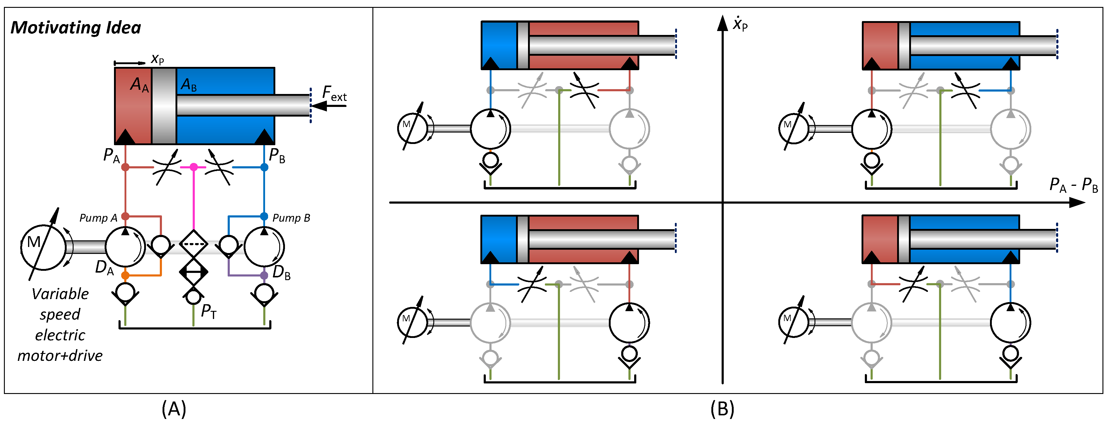
Consider the basic open circuit variable-speed drive concept in Figure 2, motivated by the premise discussed in the Introduction. Assuming no restrictions on pump port pressures and the proportional valves leakage free, this concept fundamentally differentiates itself from existing pump controlled cylinder drives by being self-locking, separating forward and return flow paths, with the latter being common for both cylinder chambers. The impact of these features is outlined below.
- Self-locking capability
- The drive concept is ideally self-locking, i.e., if the electric motor and the valves are not actuated, the cylinder piston is ideally locked. Hence, at stationary situations, the pump leakage balances the pressure difference across each pump, such that the common pump shaft is not loaded, and no energy consumption takes place. Hence, the self-locking feature allows to realize zero energy consumption when stationary (ideally). However, in the presence of even a small leakage the drive is not self-locking, but the leakage level may be significantly reduced compared to existing pump controlled drives as this is dictated by the valve and not the pump. In this case the drive may be referred to as a quasi self-locking drive.
- Separate forward & return flow paths
- This feature allows to control the pressure level of the cylinder, i.e., the lower chamber pressure. This in turn allows to control the cylinder drive stiffness, hence broadening the application range of the drive concept as discussed in the Introduction. On the other hand, this feature does not allow to regenerate energy when an external force is aiding the piston motion, and the power transferred by the load will be dissipated as heat in the drive. However, when the cylinder is supposed to carry out work, i.e., when the load is resistive, the power transmission can be rather efficient as the fluid is passed directly to the cylinder via the pump.
- Common return flow path
- The return flow passes a valve and is guided via a common path to the reservoir, allowing for cooling and filtration of the fluid. If realized properly, the fluid may be maintained in its design range regarding purity and temperature, hence viscosity, pivotal to the durability and reliability of the fluid itself, as well as the components. Note furthermore that the fluid may be circulated from the reservoir via a pump and valve through the filtering and cooling path, while maintaining the piston position and hydraulic output force constant.
It may be evident that the announced properties are strongly dependent on the drive controls. In fact, the drive is a multi-input system, a feature that is inherent due to the self-locking feature and the separate flow paths. Hence, this concept induces a large degree of freedom in the drive control, and allows to meet various objectives in terms of stiffness, cooling, filtering, efficiency, etc., if intelligent controls are developed. As the component types considered, i.e., pumps, control valves, check valves, electro motors and associated drives are readily available in large ranges, the drive concept is highly scalable. Hence, if realized at low cost, controlled properly such that operation meets the properties discussed above, while being efficient, the concept falls under the premise discussed in the Introduction, and constitutes an alternative to conventional valve solutions in a broad range of applications.
Realizing a Class of Drive Architectures with Self-Locking Capability
Several drive architectures may potentially be realized encompassing the main features of the drive concept above, and Figure 3 illustrates six of such architectures. Here architectures (A), (B), and (C) follow the basic principles of the drive concept above, with cooling and filtering in the common return line and no ability to recover energy in case of aiding loads. Architectures (D), (E), and (F) are similar to (A), (B), and (C), however these are modified with auxiliary valves such that energy related to aiding loads may be recovered to some extend. Furthermore, architectures (C) and (F) may be realized with standard components, e.g., external gear motors, and architectures (B) and (E) may be realized with standard components in terms of, e.g., external gear pumps. Architectures (B), (C), (E), and (F) are all characterized by having flow rectification between the flow source(s) and the cylinder chambers, meaning that pressure needs to build up in front of the flow source(s) before actuation of the cylinder can occur. This will induce some lag in the response of the drive, which may be diminished by reducing the volume between the flow source(s) and the flow rectifying check valves, combined with proper controls. Architectures (A) and (D) do not have these features as the pump outlets are directly connected to the cylinder chambers, and no pressure build up phase is required prior to actuation of the cylinder. However, these architectures require that the pumps allow high pressure on their suction side while avoiding a case drain. Such features are generally not available with standard components, however, with the developments within high pressure rotary sealing solutions (https://fluidpowerjournal.com/2018/10/trelleborg-announces-new-rotary-seal-high-pressure-oil-gas-applications/ (Date: 5 December 2018)), modifications of standard pumps, e.g., external gear pumps, may allow such operation modes.
3. Loss Analysis, Recovery Potential & Comparison with Conventional Valve Solutions
In the following, the losses of the proposed drive architectures are analyzed in perspective of the intended operation, i.e., assuming that proper control may be realized. Furthermore, the energy recovery potential of the drives in Figure 3D–F is investigated, followed by a comparison with conventional valve solutions. The following adopts notation for the different architectures in Figure 3 (DPCS, DPCS-R, DPDS, DPDS-R, etc.) and the nomenclature of Figure 2A, assuming check valves, filter and cooler loss free, the controllable valves leakage free, and the reservoir pressure negligible, i.e., [bar]. The pump model used is the so-called Wilson model [33]. The laminar leakage term of this model may provide a conservative description of the steady state flow losses in, e.g., external gear pumps [27], and combined with its simplicity this model is beneficial to apply here. Furthermore, the lower chamber pressure is denoted , and the load pressure , where in the absence of cylinder friction. Moreover, the conventional four quadrant diagram commonly used to classify drive operation is applied in an extended form in order to cover all relevant operation modes, and is designated extended four quadrant diagram, even though it divides the operation area into nine parts. Note that under the above conditions, the analyses of architectures (C) and (F) are identical to those of architectures (B) and (E) for , and for this reason omitted in the following.
3.1. Loss Analysis of Drive Architectures without Energy Recovery Ability
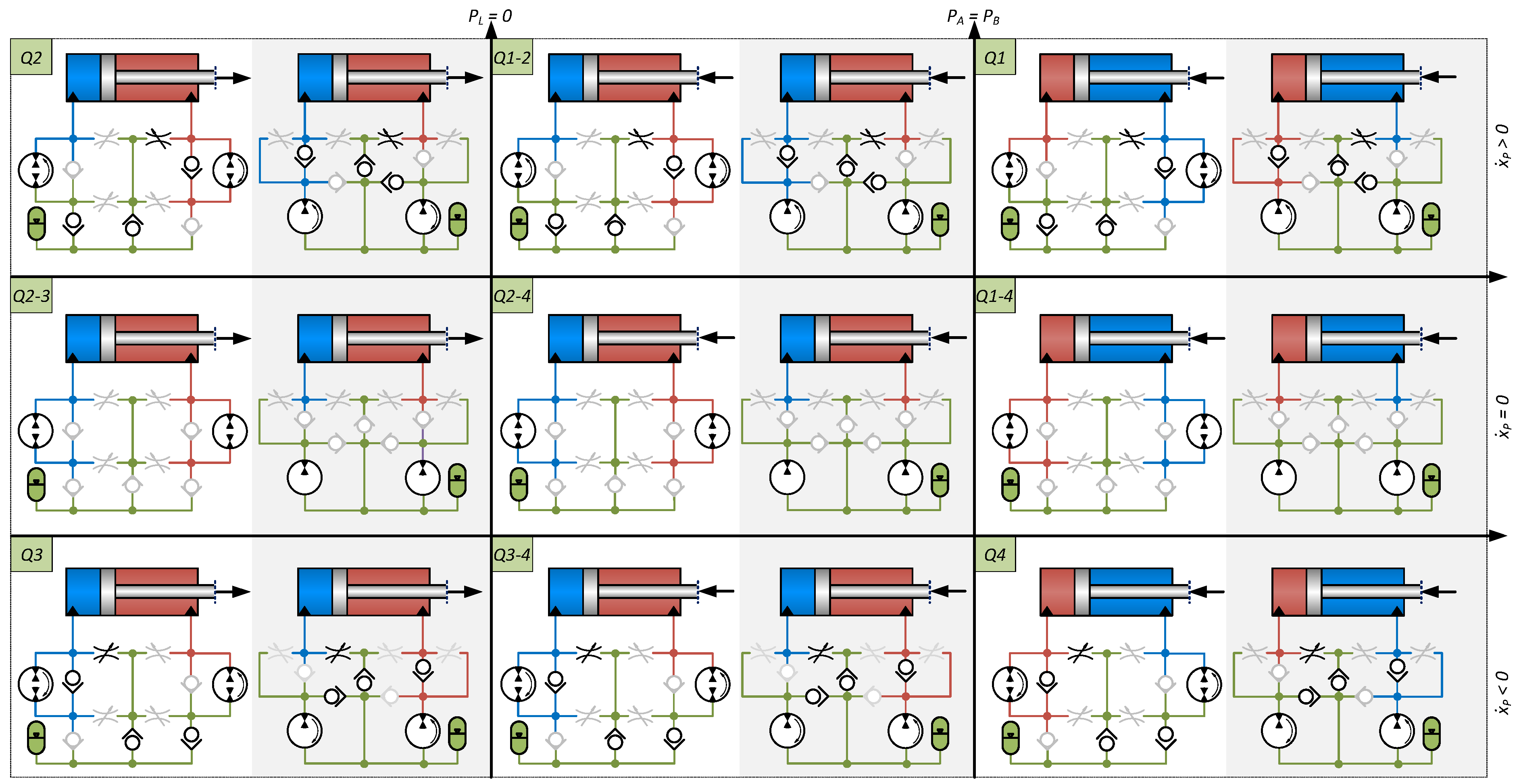
The characteristics of the drive architectures in Figure 3A–C may be considered in a steady state, as depicted in the schematics of Figure 4. The extensions to a classic four quadrant diagram include piston motion cases where the sign of the chamber pressure difference opposes that of the load pressure (Q1-2 and Q3-4) and cases with no piston motion (Q2-3, Q2-4, and Q1-4).
It may be observed from Figure 4 that if the auxiliary valves are disregarded, the operation characteristics for all architectures in Figure 3 are coincident under the ideal check valve assumption. Hence, a unified steady state energy analysis for all architectures may be established for this case.
Let and denote the power transferred via the electric motor shaft and the cylinder piston, respectively, which in any case are defined as and . Disregarding the auxiliary valves, the steady state motor shaft power for all architectures are given by Equation (1) in quadrants Q1, Q1-2, Q2 and by Equation (2) in Q3, Q3-4, Q4, where , denote the Wilson model leakage coefficient of pumps A and B, respectively.
In quadrants Q1 and Q4 i.e., and , and in remaining quadrants , . Bearing in mind signs of the load pressure and piston speed, the steady state electric motor shaft power may be described in each quadrant by Equations (3)–(8).
For quadrants Q2, Q3-4, and Q4 (Figure 4), the power transferred to the drive by the load is passed through a valve directly to the reservoir, and hence not recovered but converted to heat in the drive. However, it should be noted that the power is nearly free of cost, as the generated heat only needs to be removed in a cooling process.
As already discussed, the lower chamber pressure may be controlled via the valves, and if increased the stiffness is increased, but so are the losses due to the increased pressure difference between the lower pressure and the reservoir.
3.2. Energy Recovery Potential
In the following the energy recovery potential when using the auxiliary valves is evaluated. As opposed to the previous subsection, the remaining controllable valves are here disregarded, and the extended four quadrant diagram therefore appear as depicted in Figure 5.
Assuming the auxiliary valves sufficiently large, such that the power loss resulting from associated throttling may be considered negligible, the steady state power transmission via the electrical motor shaft for all quadrants is given by Equation (9).
In quadrants Q4 and Q2, it is possible to recover energy if the electrical system allows this, and from the above the recoverable power is bounded by Equation (12).
If the electrical system does not allow energy recovery, needs to be dissipated in a brake resistor when the drive only uses the auxiliary valves. Alternatively, the utilisation of all valves simultaneously may allow to avoid this.
It is evident from the analysis above, that if the ratio of the geometric pump displacements is equal to the piston area ratio, i.e., if , the least possible losses occur. Hence, from an efficiency point of view, this is the more feasible choice of pump displacement ratio.
3.3. Comparison with Conventional Valve Solutions
A conventional valve drive solution may generally be depicted as in Figure 6. The valve port flows are given by Equations (13) and (14) for positive and negative spool position, respectively.
To achieve the best possible efficiency with such a solution, the supply pressure may be controlled to the necessary level, which is dictated by the relation between the valve flow ports and the load of the cylinder. Assuming a steady state, leakage absent and [bar], then using and the required supply pressure is given by Equations (15) and (16).
3.4. Summary of Energy Analysis
The results of the above analyses are summarized in Table 1. From this it is found that losses of a conventional valve drive with ideal supply pressure control as well as the losses of the proposed drive architectures when using the transmission line valves, are functions of the piston speed. In the latter case this dependency may be decreased if the lower pressure is controlled to a low level, which on the other hand induces a low drive stiffness. For the former case, this feature may only be achieved in quadrants Q1 and Q3. The losses of the proposed drive architectures when utilizing the auxiliary valves only are proportional to the square of the cylinder force, and ideally independent of the piston speed. Furthermore, in these cases losses are only related to pump leakage, and therefore likely significantly lower than in the remaining cases.
4. Dynamic Modeling, Basic Controls & Performance
In order to demonstrate the properties of the proposed drive architectures in operation, a basic model based control design is realized and the performance evaluated via simulation, with a specific application used as target for the study.
4.1. Application Subject for Study
The application used for study is the test bench used in [27], being two cylinders mounted back-to-back and connected to a slide with an inertia load. One cylinder is subject for actuation by the proposed drive architectures, whereas the other cylinder functions as a load to the first cylinder (for details consult Appendix A). In the following the load cylinder is assumed an ideal force source, and hence the application is in-line with the schematics of Figure 7. The parameters from verified models of this application are used in the following, and may be found in Appendix A.
4.2. Modeling
Consider the drive architectures of Figure 3D,E, i.e., a self-locking and self-contained dual pump drive with compressed suction side and decompressed suction side, respectively, with the notation as depicted in Figure 7. In the following the DPCS-R and DPDS-R architectures are considered without the transmission line valves.
Evidently, the drive architectures share the describing equations for the cylinder motion, the check valves, the transmission line valves and volumes, the reservoir volume, and the actuator dynamics. These common describing equations are given by Equations (25)–(33), where Equations (31)–(33) describe the valve and motor/drive dynamics.
The pressure dynamics and pump flow equations, on the other hand, are different for the two drive architectures and briefly outlined in the following.
4.2.1. Hydraulic Model—DPCS/DPCS-R
4.2.2. Hydraulic Model—DPDS/DPDS-R
4.3. Basic Control Design
Consider the cases for the drive architectures, where only the auxiliary valves are used and these are fully open. Here the drives are as such operational, however with the lower pressure uncontrolled. This renders the drive stiffness uncontrolled, but also allows for power regeneration due to the non zero pump pressure differences and oppositely oriented pump torques.
In the cases where the auxiliary valves are not used, the return flows need to be guided via the transmission line valves to the reservoir, allowing for control of the lower transmission line pressure and hence control of the drive stiffness, but with no possibility for power regeneration. Such controls are designed in the following, and realized by simple proportional control action.
4.3.1. Model Simplification for Use in Control Design
As the control objective is to guide the return flow to the reservoir while maintaining a certain lower transmission line pressure, consider again the schematics of Figure 7. Assuming the check valves ideal and the reservoir pressure constant then , , and for the DPCS architecture and , for the DPDS architecture. From this it may be evident that in a steady state motion, the dynamic equations for the architectures are identical, and may be described by Equations (44) and (45) in quadrants Q1, Q1-2, Q2 and by Equations (46) and (47) in quadrants Q3, Q3-4, Q4.
4.3.2. Linear Model
The simplified model Equations (25), (44)–(47) and the valve controls Equations (48) and (49) may be expressed in a linear form as Equations (50)–(56) and Equation (31), noting that is assumed constant, introducing and assuming that . Furthermore, to avoid misinterpretation, denotes the change variable of a flow and denotes the change variable of a pressure .
In the above, linearisation constants are given by Equation (57).
4.3.3. Dynamic Analysis & Control Design
Bearing in mind that the lower pressure to be controlled is in quadrants Q1, Q4, whereas it is in quadrants Q2, Q1-2, Q3-4, and Q3, one may establish the transfer functions from the pressure control inputs , to the relevant pressures , as Equation (58) assuming a constant lower pressure reference, external force, and motor speed, noting that except on the axes of the quadrant diagram and that , .
By inspection, one may by find that poles of and are identical and that the poles of and are identical, and count two complex conjugate pairs and a real pole in all cases. Furthermore, and include two zeros (with negative real parts), whereas no zeros are included in and .
The pole variations as functions of the piston position are depicted in Figure 8, from which it is seen that the transfer from pressure control inputs to pressure outputs remains stable over the entire piston stroke with the proposed valve control inputs. Based on these properties and the fact that the pressure control accuracy is not pivotal for the drive performance, a proportional control gain is designed in a conservative way aiming at phase margins of ≈ (here this results in gain margins in the range ≈20–35 [dB], considering all four quadrants).
4.4. Drive Performance
The performance of the proposed drive class including the designed controllers is evaluated based on the same model parameters as above. First the basic properties of the drives DPDS and DPCS, where the auxiliary valves are not used, i.e., , are demonstrated when subjected to steps in the motor speed. Secondly, performance of the drives are evaluted when subject to a specific motion trajectory, and subjected to external load forces and different sizes and signs such that operation in the entire operation can be evaluated.
4.4.1. Basic Properties
The basic properties of the drives in terms of the self-locking and the non power consuming stationary properties are evaluated via a simple start-stop sequence. A piston velocity reference signal is passed to the drives via the filter in Equation (59). Here the step sizes are equal and given by = 20 [mm/s].
The results are depicted in Figure 9. The position variaton as a result of the step sequence is similar for both drives. Considering the DPDS, it may be observed that with stationary piston position, both pump outlet pressures , converge to the reservoir pressure , i.e., the pressure differences across the pumps converges to zero. Hence, the pump shaft torque converges to zero, and the electric motor is not carrying the load and hence no electrical losses would be present. However, the chamber pressures remain on levels dictated by the pressure setting and the external load , demonstrating the self-locking feature of the drive. The same behavior is seen for the DPCS, however here , converge to the corresponding line pressures, causing the pump pressure differences to converge to zero similar to the DPDS.
4.4.2. Motion Performance & Energy Efficiency
The performance of the proposed drive architectures is evaluated in regard to motion and energy efficiency and compared to a conventional valve solution as described in Section 3.3, resulting in Equation (60) when assuming the reference supply pressure transferred to the supply pressure with critically damped second order dynamics. Furthermore, the following two cases are considered for the valve solution. A case with [bar] denoted VCD, and another case with [bar] denoted VCD-R, corresponding to a high stiffness case and an energy efficient case, respectively.
To evaluate the motion performance in general a simple motion trajectory is used, given by Equation (61) combined with Equation (59), where [mm/s] and [mm/s], respectively.
This allows for motion in both directions ( and ) covering the majority of the piston range. Furthermore, five load cases are considered, i.e., where the external load force is either [kN], [kN], [kN], [kN] or [kN], thereby covering operation in quadrants Q1, Q2, Q3 and Q4. The resulting evaluation modes are denoted according Table 2.
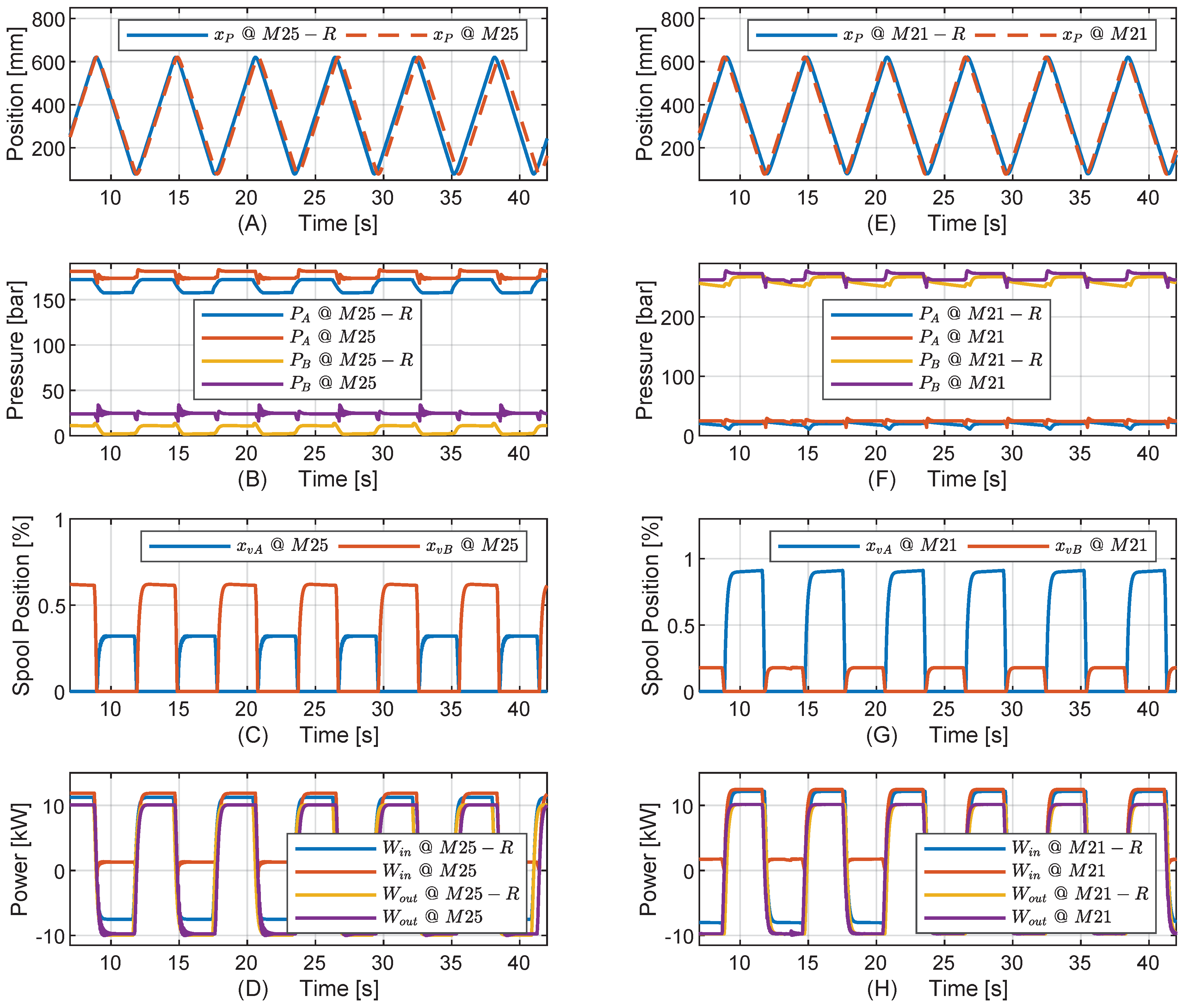
The results for the DPDS-R/DPDS drives, the DPCS-R/DPCS drives, and the VCD-R/VCD drives are depicted in Figure 10, Figure 11 and Figure 12, respectively. As may be evident, the pressure control loops of the DPDS and DPCS drives operate as intended, allowing to maintain the lower pressure level in the vicinity of the reference pressure setting = 25 [bar], whereas the lower pressures for the DPDS-R and DPCS-R drives are prone to attain lower pressure levels. As a result of the lower pressure levels for the DPDS-R and DPCS-R drives, the drive stiffnesses are significantly lower than for the DPDS and DPCS drives, however, the power consumption is on the other hand decreased.
It may be seen that in motion aiding load cases, the DPDS and DPCS drives consume energy even though no work is carried out by the cylinder piston. This is due to charging of the low-pressure chambers to the set pressure. Furthermore, all the power asserted by the load to these drives is converted to heat through throttling over the return flow valve. Hence, the high stiffness achieved by maintaining the lower chamber pressure at a certain setting, results in a low efficiency.
The DPDS-R and DPCS-R drives, on the other hand, allow the return flow to be passed to the reservoir via a pump, avoiding the main throttling losses and causing a pressure drop over the return flow pump producing a torque counter acting the forward flow pump which in turn allows for energy recovery, as also evident from the figures. Furthermore, the reduced shaft torque resulting from these pump pressure differences, will result in reduced ohmic losses in the electric motor as compared to the DPDS and DPCS drives. As may be found from Figure 10D,H and Figure 11D,H, the input and output power for the DPDS and DPDS-R drives resembles those of the DPCS and DPCS-R drives, respectively.
Considering the VCD and VCD-R solutions in comparison, no energy recovery is possible. Here both the return and forward flows are throttled over the valve, resulting in losses that are inherently dependent on the valve flow port relations and the supply pressure. Furthermore, in the case considered here the supply pressure is controlled in an ideal way such that this always is at the required level. However, a pump often supplies numerous valves not necessarily allowing for such an ideal control of the supply pressure matching all the supplied valves. Hence, generally one must expect larger losses for such valve drives than illustrated in Figure 12.
In regard to the efficiency of the proposed drive architectures, this is here considered as the ratio of the work conducted by the cylinder piston and the energy consumed by a drive, assuming that no energy is recovered electrically. Furthermore, in Equation (62) in all cases, for the DPCS, DPCS-R, DPDS, and DPDS-R drives and for the VCD and VCD-R drives for and for .
The results with operations as depicted in Figure 10, Figure 11 and Figure 12 over the course of [s] are summarized in Table 3. Here only minor differences in the efficiency are seen for the DPCS and DPDS drives and the DPCS-R and DPDS-R drives, respectively. Furthermore, these drives show lower efficiencies for operation in Q3, Q3-4, Q4 than operation in Q1, Q1-2, Q2, which is due to increased pump leakage and valve throttling losses resulting from the relatively higher pressure level when . Generally, the DPCS, DPDS, DPCS-R, and DPDS-R drives demonstrate highly improved efficiency compared to the VCD and VCD-R cases, even when the supply pressure is controlled in an ideal way. Only the VCD-R drive shows an increased efficiency at [kN], however here no work is carried out by the cylinder.
5. Industrial Feasibility Study
Having considered technical matters in terms of energy analysis, basic controls, and performance for the proposed drives, their industrial feasibility is considered. Here industrial feasibility refers to the application range and scalability of the proposed drive(s), their reliability and durability, as well as cost of realization.
5.1. Application Range & Scalability
In general, if based on standard components, the application range is large for the proposed class of drives. This is evident when considering the usage of induction machines and fixed displacement axial piston machines, with ranges up to hundreds of [kW] and [cmrev], respectively. Taking into account the commercial aspects however, it is resonable to consider, e.g., external gear machines, induction machines, and simple 2/2 valves in regard to the proposed drives.
As an example, consider the standard Bosch Rexroth external gear pump series AZPF and AZPG, standard check valve series M-SR for block mounting, and standard 2/2 proportional valve series KKDSR1 and KKDSR2, having nominal flow ranges of [L/min] and [L/min], respectively.
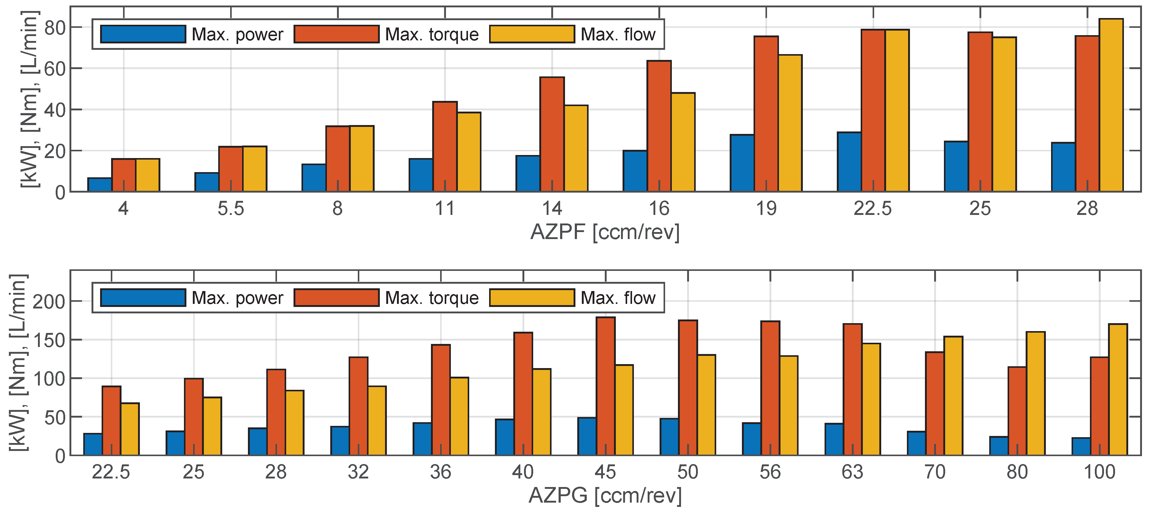
For the drives proposed here, each pump should be accompanied by two check valves as well as one (or two) proportional valves with corresponding flow capacities. Evaluating the pump series in consideration, one may establish flow, torque, and power ranges, as depicted in Figure 13.
Hence, considering only these standard external gear pumps, one may realize drives with nominal (input) power up to ≈[kW], shaft torques up to ≈[Nm], and nominal flows up to ≈[L/min]. In the latter case, three of the considered valves would be required to realize the flow capacity of “one” valve as mentioned above. This may however also be realized with other valve types.
Reliability & Durability
A fundamental requirement to a hydraulic drive (and hydraulic systems in general) for this to be reliable and durable is that its components and the hydraulic fluid are kept within design ranges. Essential to the wear of both components and fluids is the temperature and contamination level, and the possibility of the proposed drives to guide the return flow through the common return line allow to control these properties via conventional cooling and filtering functionalities. For architectures (A), (B), (C), and (D) in Figure 3, the return flow in passing the common return line inherently, whereas architectures (E) and (F) allow for this, dependent on the controls. The only challenge in the usage of components is that the pumps in the architectures of Figure 3A,D and Figure 3B,E are operated in four or two quadrant operation, respectively. In regard to two quadrant operation (±speed operation), this has been considered in industry [20] and in research studies [21,25,27], and no problems with this type of operation have been reported. The four quadrant operation of pumps without drains is not realizable with standard components, however, modifying the sealing solutions in existing pumps may allow to realize this, as discussed in Section 2.
5.2. Realization Cost
In order to investigate the cost efficiency of the proposed drive class, the combined cost of main individual components is compared to that of a conventional drive solution. For conservativeness, dual pump architectures that include auxiliary valves are considered, i.e., drive architectures DPCS-R and DPDS-R of Figure 3. These are compared to a conventional valve drive, based on a conventional proportional valve (here a Bosch Rexroth type 4WRSEH), disregarding the related piping for conservativeness. Furthermore, this comparison is made for two cases of rated drive (input) power being [kW] and [kW], respectively.
The study is based on main components, where electric cabinets, wiring, etc. are assumed to be of equal cost in all cases, and therefore not included. Also, components are chosen from basic static calculations on flows, pressures, shaft torques targeting piston area ratios of . The resulting components are outlined in Table 4.
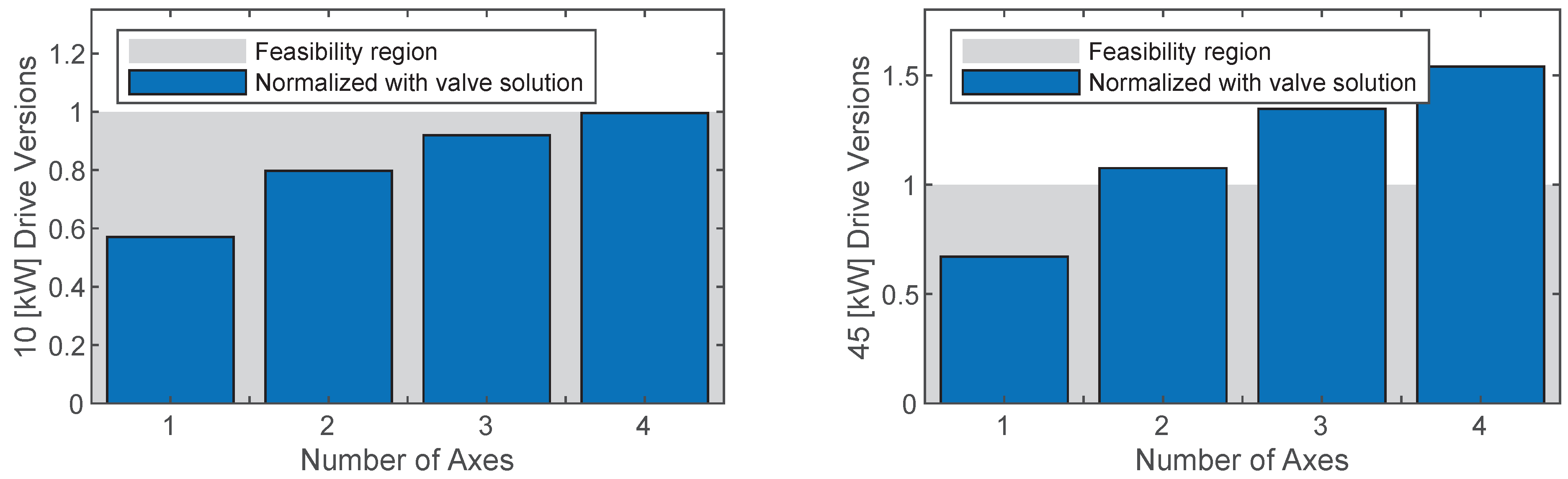
Hydraulic power units are commonly shared by several axes. Hence, for the sake of conservativeness, the comparison is made when considering 1–4 cylinder axes, all sharing the same hydraulic power unit (here designed for a single axis, i.e., it is assumed that only one axis is in motion at a time). The cost for n self-contained drives normalized with n conventional drives is evaluated from Equation (63) for .
Hence, for a normalized cost below one, a solution with one of the proposed drive architectures has a lower cost than a conventional solution, and oppositely for a normalized cost above one. The results are outlined in Figure 14 (note that all cost information used as basis for these results originate from Bosch Rexroth, Denmark.).
An obvious drawback of the proposed drives as compared to conventional valve solutions is the necessity for an electric motor and associated electric drive for each cylinder axis. The cost of such components increases somewhat more with increased power range as compared to conventional 4/3 valves. Here the same valve housing typically covers large flow ranges at the same pressure range (hence large power range), where the only difference is the geometry of the valve spool. Hence the increased flow range only has little or no influence on the cost when considering a specific valve type, whereas an increased flow range in a pump operated drive requires a larger electric motor for each drive. On the other hand, an advantage of self-contained drives compared to conventional valve solutions is the reduced necessity for piping. Pipes and their installation process is typically associated with substantial cost (Bosch Rexroth, Denmark), depending on the distance between the hydraulic power unit and the cylinders it supplies, the number of pipe bends, etc. at the site of installation. Even though the cost of piping may be substantial, this is difficult to include in the cost comparison, as this strongly depends on the application, the installation site layout, etc.
As evident from above, the proposed drives demonstrate a commercial potential which is dependent on the power size and the number drives to be used. Together with the possibility to realize the proposed drives on a large scale, the range of application resulting from the range of component sizes and controllable drive stiffness, as well as the energy efficiency, generally causes these to be industrially feasible.
6. Conclusions
A class of self-locking, self-contained, and pump controlled hydraulic cylinder drives is proposed, taking offset in the idea of establishing a drive around a hydraulic lock. Six different drive architectures based on this idea are proposed, separating the forward and return flow lines such that the cylinder input flows are realized with rectified pump outlet flows, and the cylinder return flows via valves through common returns line to the reservoir. The latter feature allows for cooling and filtration of the entire cylinder return flow, while allowing the lower pressure level to be controlled to a certain level due to return flow throttling. This allows to maintain the operation of the drive components and the fluid within their design ranges, hence the reliability and durability of the components and hence the drive itself. On the other hand, this feature does not allow for energy regeneration, which is why three out the six proposed drives are equipped with additional valves allowing to bypass the pump outlet flow rectification, and guide the return flow via the corresponding pump to the reservoir such that power can be regenerated in motion aiding load cases. The proposed class of drives was analyzed in regard to power losses and energy recovery potential, with the analytic results compared to those of a conventional valve controlled hydraulic drive architecture assuming that the valve supply pressure may be controlled in a ideal manner, demonstrating the energy efficiency potential of the proposed drive class. As the proposed drive class cannot function if the return flow is not controlled properly, basic controls enabling this are designed in a model based way. Simulation results with physical parameters taking offset in an experimentally verified test bench demonstrate proper motion performance, lower pressure level control, and furthermore superior energy efficiency in the majority of the operating range when compared to that of a conventional valve solution. Finally, the industrial feasibility of the proposed drive class was considered in terms of application range, scalability, reliability/durability, and cost of realization. It was found that the operation within component design ranges, that standard component size range and controllable drive stiffness, causes the proposed class of drives to have a large application range, to be reliable and to be scalable up to at least [kW] with utilization of gear pumps, and higher with, e.g., axial piston pumps. Finally, based on actual component costs, it was found that the proposed drive class can be cost competitive with conventional valve solutions up to [kW], when utilizing standard off-the-shelf components.
Author Contributions
Conceptualization, L.S., S.K., K.A.M. and M.H.B.; methodology, L.S.; investigation, L.S.; resources, L.S., S.K., K.A.M. and M.H.B.; writing—original draft preparation, L.S.; writing—review and editing, L.S., S.K., K.A.M. and M.H.B.; visualization, L.S.; funding acquisition, L.S., K.A.M.
Funding
This research was funded by the Danish Energy Agency, the Energy Technology Development and Demonstration Programme, project: Energy Efficient and Self-contained Hydraulic Drive Concept (SenDrive), project number 64018-0094.
Conflicts of Interest
The authors declare no conflict of interest.
Appendix A
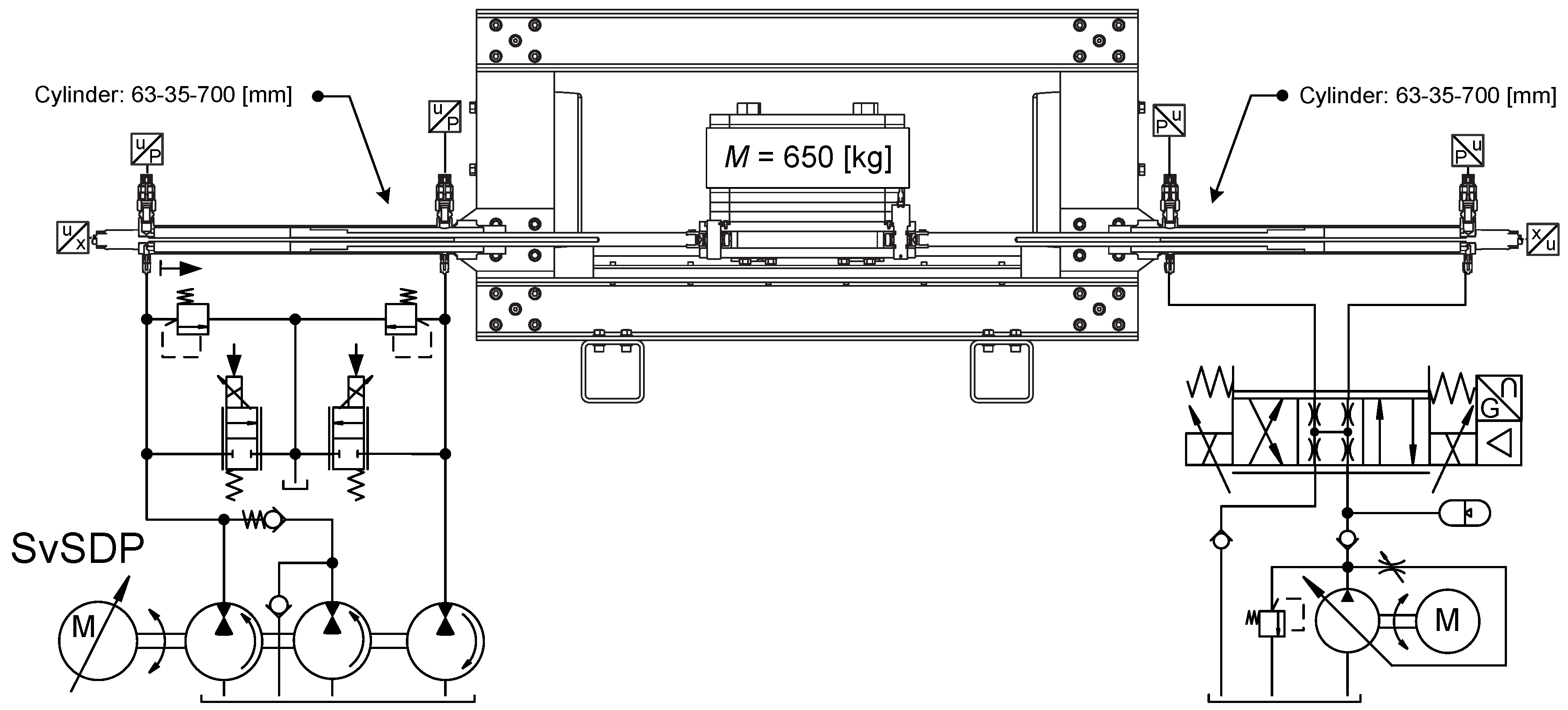
Test bench subject for analysis and control designs, when mounted with the DPDS-R, DPCS-R, DPDS, and DPCS drives instead of the SvSDP drive concept.
Figure A1.
Test bench with the so-called Speed-variable Switched Differential Pump (SvSDP) prototype drive (Aalborg University, Denmark) [27].
Figure A1.
Test bench with the so-called Speed-variable Switched Differential Pump (SvSDP) prototype drive (Aalborg University, Denmark) [27].

Besides the model described in Section 4, the effective bulk modulii for the fluid-air mixture , A, B, AT, BT, R, T are described by Equation (A1) [34] and the pump shaft torque of the DPCS, DPDS, DPCS-R, and DPDS-R architectures is described by (A2).
Furthermore, the parameters used are presented in Table A1.

Table A1.
Parameters for testbench and additional parameters used in analysis and simulation study.
| Verified Parameters from Test Bench | |||
| Parameter | Value | Unit | Description |
| [cm] | Piston side (A-side) area. | ||
| [cm] | Rod side (B-side) area. | ||
| 6480 | [Ns/m] | Viscous friction coefficient. | |
| [L/min/bar] | Leakage coefficient for pump A. | ||
| [L/min/bar] | Leakage coefficient for pump B. | ||
| [L/rev] | Theoretical displacement of pump A. | ||
| [L/rev] | Theoretical displacement of pump B. | ||
| [Nm] | Coulomb friction coefficient of pump A. | ||
| [Nm s/rad] | Viscous friction coefficient of pump A. | ||
| [Nm/bar] | Directional dependent load torque coefficient of pump A. | ||
| [Nm/bar] | Load torque coefficient of pump A. | ||
| [Nm] | Coulomb friction coefficient of pump A. | ||
| [Nm s/rad] | Viscous friction coefficient of pump A. | ||
| [Nm/bar] | Directional dependent load torque coefficient of pump A. | ||
| [Nm/bar] | Load torque coefficient of pump A. | ||
| 700 | [mm] | Piston stroke. | |
| M | 658 | [Ns/m] | Mass of piston and load. |
| [bar] | Athmospheric pressure. | ||
| [L] | Volume of A-side chamber with fully retracted piston. | ||
| [L] | Volume of B-side chamber with fully retracted piston. | ||
| 0.69 | [-] | Cylinder Area Ratio. | |
| 7500 | [bar] | Maximum effective bulk modulus. | |
| Percentage air in the fluid. | |||
| Adiabatic constant. | |||
| [rad/s] | Small signal bandwidth of electroc motor + drive. | ||
| [rad/s] | Small signal bandwidth of 2/2 valves. | ||
| Damping ratio of electroc motor + drive. | |||
| 0.69 | [-] | Valve flow gain ratio. | |
| 1 | Damping ratio of 2/2 valves. | ||
| Additional Parameters Used in Simulation Study | |||
| Parameter | Value | Unit | Description |
| [L/min/] | Static valve flow gain. | ||
| [L/min/] | Static valve flow gain. | ||
| [L/min/] | Static check valve flow gain. | ||
| [L/min/] | Static check valve flow gain. | ||
| [L] | Accumulator volume. | ||
| [L] | Volume between pump A and related check valves. | ||
| 1 | [L] | Return line volume. | |
| [L] | Dead volume of accumulator and related connections. | ||
References
- Ketelsen, S.; Padovani, D.; Andersen, T.; Ebbesen, M.; Schmidt, L. Classification and Review of Pump-Controlled Differential Cylinder Drives. Energies 2019, 12, 1293. [Google Scholar] [CrossRef]
- Berbuer, J. Neuartige Servoantriebe mit Primärer Verdrängersteuerung. Ph.D. Thesis, RWTH Aachen, Aachen, Germany, 1988. (In German). [Google Scholar]
- Rahmfeld, R.; Ivantysynova, M. Energy Saving hydraulic actuators for mobile machines. In Proceedings of the Bratislavian Fluid Power Conference, Častá-Píla, Slovakia, 2–3 June 1998. [Google Scholar]
- Rahmfeld, R.; Ivantysynova, M. Displacement controlled linear actuator with differential cylinder—A way to save primary energy in mobile machines. In Proceedings of the Fifth International Conference on Fluid Power Transmission and Control, Hangzhou, China, 4–5 April 2001. [Google Scholar]
- Rahmfeld, R.; Ivantysynova, M.; Weber, J. Displacement Controlled Wheel Loader- a simple and clever Solution. In Proceedings of the 4th International Fluid Power Conference, Dresden, Germany, 23–24 March 2004; pp. 183–196. [Google Scholar]
- Schneider, M.; Koch, O.; Weber, J. Green Wheel Loader—Improving fuel economy through energy efficient drive and control concepts. In Proceedings of the 10th International Fluid Power Conference, Dresden, Germany, 8–10 March 2016. [Google Scholar]
- Williamson, C.; Zimmerman, J.; Ivantysynova, M. Efficiency study of an excavator hydraulic system based on displacement-controlled actuators. In Proceedings of the 21st Fluid Power and Motion Control Symposium, Bath, UK, 10–12 September 2008; pp. 291–307. [Google Scholar]
- Zimmerman, J.D.; Ivantysynova, M. Reduction of Engine and Cooling Power by Displacement Control. In Proceedings of the 6th FPNI PhD symposium, West Lafayette, IN, USA, 15–19 June 2010; pp. 339–352. [Google Scholar]
- Zimmerman, J.; Busquets, E.; Ivantysynova, M. 40% fuel savings by displacement control leads to lower working temperatures—A simulation study and measurements. In Proceedings of the 52nd National Conference on Fluid Power, Las Vegas, NV, USA, 23–25 March 2011; pp. 693–702. [Google Scholar]
- Busquets, E.; Ivantysynova, M. The World’s First Displacement-Controlled Excavator Prototype With Pump Switching—A Study of the Architecture and Control. In Proceedings of the 9th JFPS International Symposium on Fluid Power, Matsue, Japan, 28–31 October 2014. [Google Scholar]
- Busquets, E.; Ivantysynova, M. A Multi-Actuator Displacement-Controlled System with Pump Switching—A Study of the Architecture and Actuator-Level Control. JFPS Int. J. Fluid Power Syst. 2015, 8, 66–75. [Google Scholar] [CrossRef]
- Bosch Rexroth AG. SHA Servo-Hydraulic Actuator. 2017. Available online: https://dc-corp.resource.bosch.com/media/general_use/products/industrial_hydraulics_1/systems_1/20170915_Kundeninformation_SHA_EN.pdf (accessed on 3 April 2019).
- Bosch Rexroth AG. Advantages of Electrification and Digitalization Technology For Hydraulics. 2018. Available online: https://www.boschrexroth.com/en/xc/products/product-groups/industrial-hydraulics/the-fitness-program-for-hydraulics (accessed on 3 April 2019).
- Padovani, D.; Ketelsen, S.; Hagen, D.; Schmidt, L. A Self-Contained Electro-Hydraulic Cylinder with Passive Load-Holding Capability. Energies 2019, 12, 292. [Google Scholar] [CrossRef]
- Imam, A.; Rafiq, M.; Jalayeri, E.; Sepehri, N. Design, Implementation and Evaluation of a Pump-Controlled Circuit for Single Rod Actuators. Actuators 2017, 6, 10. [Google Scholar] [CrossRef]
- Michel, S.; Weber, J. Electrohydraulic Compact-drives for Low Power Applications considering Energy-efficiency and High Inertial Loads. In Proceedings of the 7th FPNI PhD Symposium on Fluid Power, Reggio Emilia, Italy, 27–30 June 2012; pp. 1–18. [Google Scholar]
- Michel, S.; Weber, J. Energy-efficient electrohydraulic compact drives for low power applications. In Proceedings of the ASME/BATH 2012 Fluid Power andMotion Control, Bath, UK, 12–14 September 2012; pp. 93–107. [Google Scholar]
- Çalışkan, H.; Balkan, T.; Platin, B.E. A Complete Analysis for Pump Controlled Single Rod Actuators. In Proceedings of the 10th International Fluid Power Conference, Dresden, Germany, 8–10 March 2016; pp. 119–132. [Google Scholar] [CrossRef]
- Çalışkan, H.; Balkan, T.; Platin, B.E. A Complete Analysis and a Novel Solution for Instability in Pump Controlled Asymmetric Actuators. J. Dyn. Syst. Meas. Control 2015, 137, 091008. [Google Scholar] [CrossRef]
- Brahmer, B. CLDP—Hybrid Drive using Servo Pump in Closed Loop. In Proceedings of the 8th International Fluid Power Conference, Dresden, Germany, 26–28 March 2012; pp. 93–102. [Google Scholar]
- Minav, T.; Panu, S.; Matti, P. Direct-Driven Hydraulic Drive Without Conventional Oil Tank. In Proceedings of the ASME/BATH Symposium on Fluid Power & Motion Control, FPMC2014, Bath, UK, 10–12 September 2014; pp. 1–6. [Google Scholar] [CrossRef]
- Filatov, D.; Minav, T.; Heikkinen, J.E. Adaptive Control for Direct-Driven Hydraulic Drive. In Proceedings of the 11th International Fluid Konference, Aachen, Germany, 19–21 March 2018. [Google Scholar]
- Minav, T.; Bonato, C.; Sainio, P.; Pietola, M. Direct Driven Hydraulic Drive. In Proceedings of the 9th International Fluid Power Conference (IFK), Aachen, Germany, 24–26 March 2014; pp. 7–11. [Google Scholar] [CrossRef]
- Järf, A.; Minav, T.; Pietola, M. Nonsymmetrical Flow Compensation Using Hydraulic Accumulator. In Proceedings of the 9th FPNI Ph.D. Symposium on Fluid Power FPNI2016, Florianópolis, SC, Brazil, 26–28 October 2016; pp. 1–6. [Google Scholar] [CrossRef]
- Pedersen, H.C.; Schmidt, L.; Andersen, T.O.; Brask, M.H. Investigation of New Servo Drive Concept Utilizing Two Fixed Displacement Units. JFPS Int. J. Fluid Power Syst. 2014, 8, 1–9. [Google Scholar] [CrossRef] [Green Version]
- Schmidt, L.; Roemer, D.B.; Pedersen, H.C.; Andersen, T.O. Speed-Variable Switched Differential Pump System for Direct Operation of Hydraulic Cylinders. In Proceedings of the ASME/BATH 2015 Symposium on Fluid Power and Motion Control, Chicago, IL, USA, 14–16 October 2015. [Google Scholar]
- Schmidt, L.; Groenkjaer, M.; Pedersen, H.C.; Andersen, T.O. Position Control of an Over-Actuated Direct Hydraulic Cylinder Drive. Control Eng. Pract. 2017, 64, 1–14. [Google Scholar] [CrossRef]
- Ketelsen, S.; Schmidt, L.; Donkov, V.H.; Andersen, T.O. Energy Saving Potential in Knuckle Boom Cranes using a Novel Pump Controlled Cylinder Drive. Modeling Identif. Control 2018, 39, 73–89. [Google Scholar] [CrossRef]
- Servi Group. Servi Hybrid Drive. Linear Actuator. 2017. Available online: https://www.servi.no/media/documents/Hybrid_Cylinder_1705-1_NO.pdf (accessed on 3 April 2019).
- Michel, S.; Schulze, T.; Weber, J. Energy-efficiency and thermo energetic behaviour of electrohydraulic compact drives. In Proceedings of the 9th International Fluid Power Conference (IFK), Aachen, Germany, 24–26 March 2014. [Google Scholar]
- Michel, S.; Weber, J. Prediction of the thermo-energetic behaviour of an electrohydraulic compact drive. In Proceedings of the 10th International Fluid Power Conference (IFK), Dresden, Germany, 8–10 March 2016; pp. 219–234. [Google Scholar]
- Michel, S.; Weber, J. Investigation of Self-Contamination of Electrohydraulic Compact Drives. In Proceedings of the 10th JFPS International Symposium on Fluid Power, Fukuoka, Japan, 24–27 October 2017. [Google Scholar]
- Costa, G.K.; Sepehri, N. Hydrostatic Transmissions and Actuators: Operation, Modelling and Applications; Wiley: Hoboken, NJ, USA, 2015. [Google Scholar]
- Andersen, T.O.; Hansen, M.R. Fluid Power Systems—Modelling and Analysis, 2nd ed.; Aalborg University: Aalborg, Denmark, 2003. [Google Scholar]
Figure 1.
Examples on self-contained linear hydraulic drives. (A) Variable displacement, closed circuit drive. (B) Variable speed, closed circuit drive. (C) Variable speed, open circuit drive.
Figure 1.
Examples on self-contained linear hydraulic drives. (A) Variable displacement, closed circuit drive. (B) Variable speed, closed circuit drive. (C) Variable speed, open circuit drive.

Figure 2.
(A) Self-locking pump drive concept. (B) Four quadrant illustration of the intended basic drive operation.
Figure 2.
(A) Self-locking pump drive concept. (B) Four quadrant illustration of the intended basic drive operation.

Figure 3.
Different architectures contained in the proposed class of drives. Drives (D–F) are modifications of drives (A–C), with energy regeneration capability. The yellow valves allowing for energy regeneration are denoted auxiliary valves, whereas the white valves are denoted transmission line valves.

Figure 4.
Extended four quadrant diagram(s) for drive architectures in Figure 3, when only actuating valves connecting transmission lines to the reservoir. Schematics in shaded areas are representative for architectures DPDS-R, SPDS-R, DPDS, and SPDS, whereas the schematics in non-shaded areas cover architectures DPCS-R and DPCS.

Figure 5.
Operations schematics for drive architectures of Figure 3, when only actuating the auxiliary valves. Schematics in shaded areas are representative for architectures DPDS-R and SPDS-R, whereas the schematics in non-shaded areas are representative for architectures DPCS-R.
Figure 5.
Operations schematics for drive architectures of Figure 3, when only actuating the auxiliary valves. Schematics in shaded areas are representative for architectures DPDS-R and SPDS-R, whereas the schematics in non-shaded areas are representative for architectures DPCS-R.

Figure 6.
Schematics of a conventional valve drive solution.

Figure 7.
Drive Schematics with nomenclature used for modeling. (A) DPCS-R drive schematics. (B) DPDS-R drive schematics.
Figure 7.
Drive Schematics with nomenclature used for modeling. (A) DPCS-R drive schematics. (B) DPDS-R drive schematics.

Figure 8.
(A) Pole maps as functions of the piston position. (B,C) depict the two complex conjugate pole pairs, and figure (D) depicts the real pole. Crosses denote poles in Q1 and Q2 (and Q1-2), and squares denote poles in Q4 and Q3 (and Q3-4).
Figure 8.
(A) Pole maps as functions of the piston position. (B,C) depict the two complex conjugate pole pairs, and figure (D) depicts the real pole. Crosses denote poles in Q1 and Q2 (and Q1-2), and squares denote poles in Q4 and Q3 (and Q3-4).

Figure 9.
Results with velocity step sequence with [kN] and [bar]. (A) Piston position for DPDS drive. (B) Relevant pressures for DPDS drive. (C) Piston position for DPCS drive. (D) Relevant pressures for DPCS drive.
Figure 9.
Results with velocity step sequence with [kN] and [bar]. (A) Piston position for DPDS drive. (B) Relevant pressures for DPDS drive. (C) Piston position for DPCS drive. (D) Relevant pressures for DPCS drive.
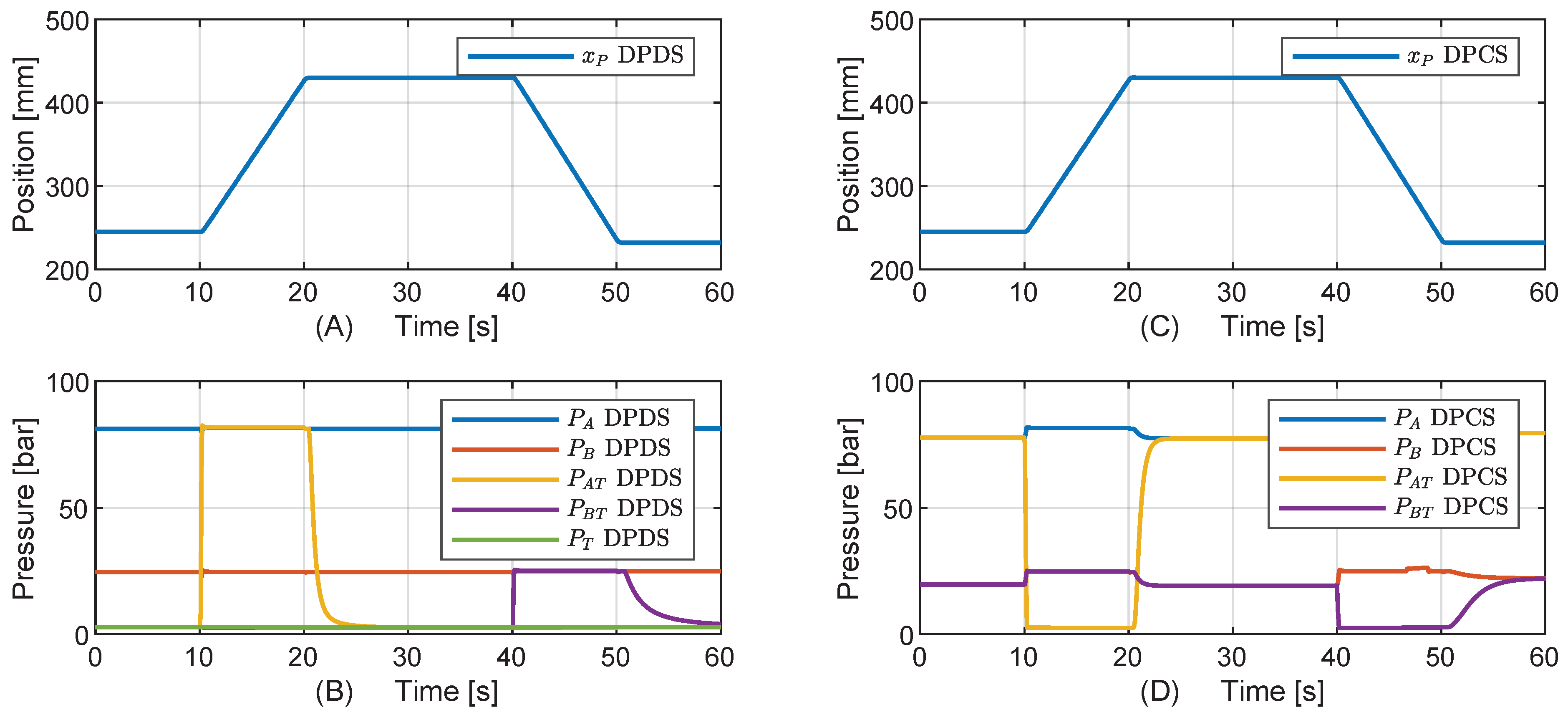
Figure 10.
Simulation results for the DPDS and DPDS-R drive architectures. (A–D) Depict the results for M25, M25-R, and (E–H) depict the results for M21, M21-R.
Figure 10.
Simulation results for the DPDS and DPDS-R drive architectures. (A–D) Depict the results for M25, M25-R, and (E–H) depict the results for M21, M21-R.

Figure 11.
Simulation results for the DPCS and DPCS-R drive architectures. (A–D) Depict the results for M25, M25-R, and (E–H) depict the results for M21, M21-R.
Figure 11.
Simulation results for the DPCS and DPCS-R drive architectures. (A–D) Depict the results for M25, M25-R, and (E–H) depict the results for M21, M21-R.

Figure 12.
Simulation results for the VCD and VCD-R drive architectures. (A–D) Depict the results for M25, M25-R, and (E–H) depict the results for M21, M21-R.
Figure 12.
Simulation results for the VCD and VCD-R drive architectures. (A–D) Depict the results for M25, M25-R, and (E–H) depict the results for M21, M21-R.
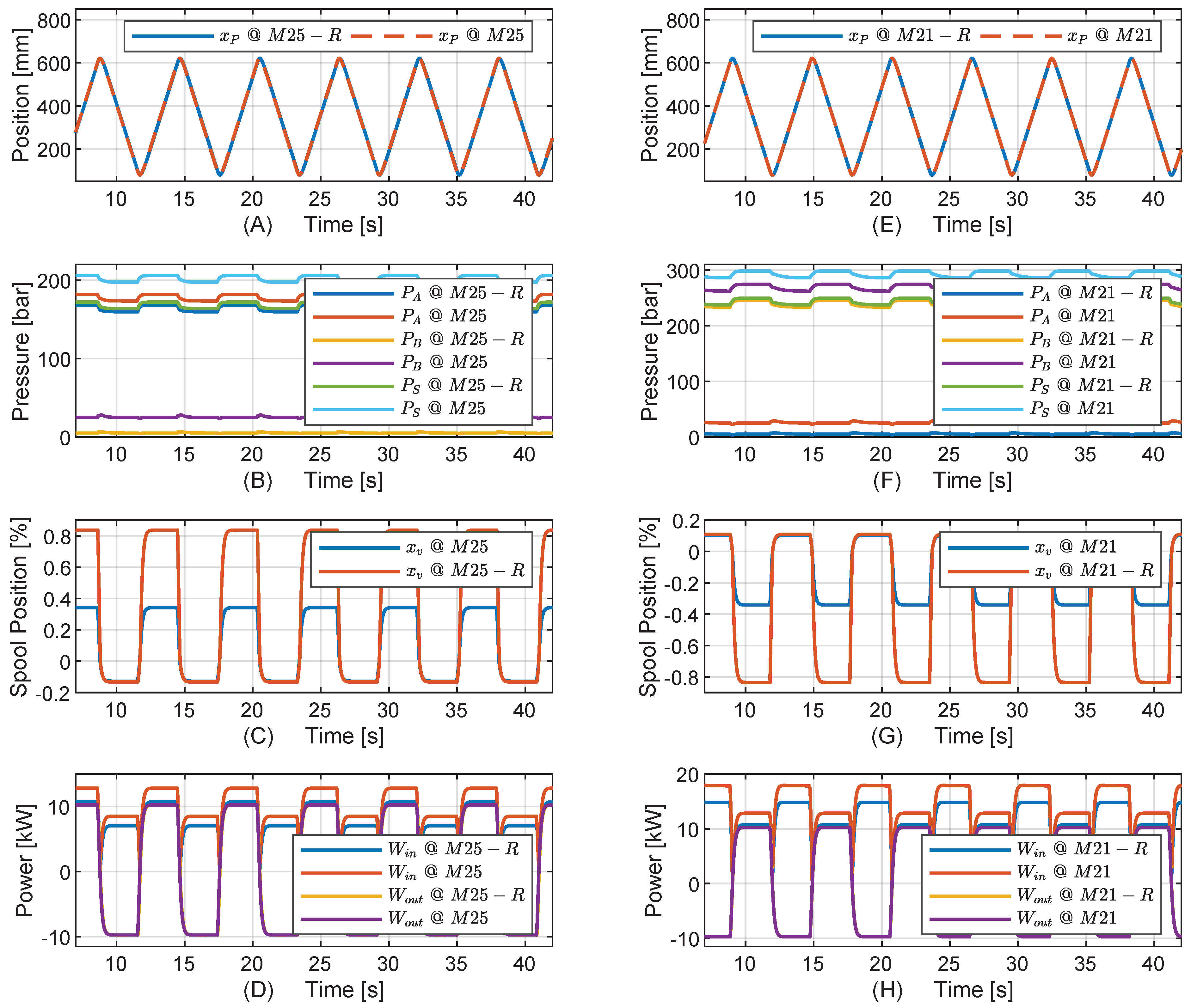
Figure 13.
Flow, torque, and power ranges for standard external gear pumps (Bosch Rexroth AZPF and AZPG), assuming ideal operation.
Figure 13.
Flow, torque, and power ranges for standard external gear pumps (Bosch Rexroth AZPF and AZPG), assuming ideal operation.

Figure 14.
Cost of proposed drive architectures DPDS-R, DPCS-R, normalized with valve solutions. Gray areas imply feasible regions, i.e., regions where drive architectures DPDS-R, DPCS-R are more cost effective than a conventional valve solution.
Figure 14.
Cost of proposed drive architectures DPDS-R, DPCS-R, normalized with valve solutions. Gray areas imply feasible regions, i.e., regions where drive architectures DPDS-R, DPCS-R are more cost effective than a conventional valve solution.

Table 1.
Summary of power losses in proposed drive architectures and conventional valve solutions.
| Quadrant | DPCS/DPDS | DPCS-R/DPDS-R @ , aux. Valves Only | Conventional Valve Solution |
|---|---|---|---|
| Power Losses | |||
| Q1: | |||
| Q1-2: | |||
| Q2: | |||
| Q4: | |||
| Q3-4: | |||
| Q3: | |||
Table 2.
Different modes considered in evaluation of the proposed drive class.
| DPCS/DPDS/VCD | |||||
| / | [kN] | [kN] | [kN] | [kN] | [kN] |
| [m/s] | M11 | M12 | M13 | M14 | M15 |
| [m/s] | M21 | M22 | M23 | M24 | M25 |
| DPCS-R/DPDS-R/VCD-R | |||||
| / | [kN] | [kN] | [kN] | [kN] | [kN] |
| [m/s] | M11-R | M12-R | M13-R | M14-R | M15-R |
| [m/s] | M21-R | M22-R | M23-R | M24-R | M25-R |
Table 3.
Ratio of piston work and drive energy consumption ().
| —DPCS/DPDS/VCD | |||||
| / | [kN] | [kN] | [kN] | [kN] | [kN] |
| [m/s] | 71/71/32 | 57/57/27 | 7/7/4 | 65/65/40 | 76/76/48 |
| [m/s] | 71/71/33 | 58/58/28 | 13/13/8 | 65/65/40 | 77/76/48 |
| —DPCS-R/ DPDS-R/VCD-R | |||||
| / | [kN] | [kN] | [kN] | [kN] | [kN] |
| [m/s] | 89/89/38 | 85/86/37 | 20/21/21 | 90/90/56 | 91/91/58 |
| [m/s] | 84/84/40 | 76/76/39 | 18/18/34 | 86/86/56 | 90/90/57 |
Table 4.
Components used as basis for commercial feasibility study. Note that all components (except for reservoirs) are included in the Bosch Rexroth standard component program. Note that the reason for the use of 8 proportional valves and associated amplifiers in the [kW] case is a result of the required flow and the valve sizes available.
| Self-Contained Drives | 10 [kW] Version | 45 [kW] Version | ||
| Pump A: | 1 pcs. | AZPF 8 ccm/rev | 1 pcs. | AZPG 45 ccm/rev |
| Pump B: | 1 pcs. | AZPF 5.5 ccm/rev | 1 pcs. | AZPG 32 ccm/rev |
| Check valves: | 5 pcs. | M-SR 8 | 5 pcs. | M-SR 20 |
| Prop. valves: | 4 pcs. | KKDSR1 | 8 pcs. | KKDSR2 |
| Valve amplifiers: | 4 pcs. | VT-SSPA-1 | 8 pcs. | VT-SSPA-1 |
| Electric motor: | 1 pcs. | MOT-FC 160M/11kW | 1 pcs. | MOT-FC 225M/45kW |
| Frequency drive: | 1 pcs. | EFC5610 11kW | 1 pcs. | EFC5610 45kW |
| Accumulator: | 1 pcs. | HAB 10 | 1 pcs. | HAB 10 |
| Conventional valve drives | 10 [kW] Version | 45 [kW] Version | ||
| Control valve: | 1 pcs. | 4WRSEH 6 | 1 pcs. | 4WRSEH 10 |
| Electric motor: | 1 pcs. | MOT-FC 160M/11kW | 1 pcs. | MOT-FC 225M/45kW |
| Power electronics: | 1 pcs. | 10 kW rating | 1 pcs. | 45 kW rating |
| Variable displacement pump: | 1 pcs. | A10VSO 18 DR | 1 pcs. | A10VSO 100 DR |
| Reservoir: | 1 pcs. | 120 L type | 1 pcs. | 585 L type |
© 2019 by the authors. Licensee MDPI, Basel, Switzerland. This article is an open access article distributed under the terms and conditions of the Creative Commons Attribution (CC BY) license (http://creativecommons.org/licenses/by/4.0/).
Share and Cite
MDPI and ACS Style
Schmidt, L.; Ketelsen, S.; Brask, M.H.; Mortensen, K.A. A Class of Energy Efficient Self-Contained Electro-Hydraulic Drives with Self-Locking Capability. Energies 2019, 12, 1866. https://doi.org/10.3390/en12101866
AMA Style
Schmidt L, Ketelsen S, Brask MH, Mortensen KA. A Class of Energy Efficient Self-Contained Electro-Hydraulic Drives with Self-Locking Capability. Energies. 2019; 12(10):1866. https://doi.org/10.3390/en12101866
Chicago/Turabian StyleSchmidt, Lasse, Søren Ketelsen, Morten Helms Brask, and Kasper Aastrup Mortensen. 2019. "A Class of Energy Efficient Self-Contained Electro-Hydraulic Drives with Self-Locking Capability" Energies 12, no. 10: 1866. https://doi.org/10.3390/en12101866
Note that from the first issue of 2016, this journal uses article numbers instead of page numbers. See further details here.