Investigation on Dynamic Response of Grid-Tied VSC During Electromechanical Oscillations of Power Systems

Abstract

This study focuses on the dynamics of a grid-tied voltage source converter (GVSC) during electromechanical oscillations. A small-signal model with GVSC port variables (DC voltage and AC power) as the outputs and a terminal voltage vector as the input is derived to reveal the passive response of the GVSC on the basis of the power equation in the d–q coordinate system. An input–output transfer function matrix is constructed according to the proposed model. The frequency response of this matrix in the electromechanical bandwidth is described to reflect the dynamic behavior of the GVSC. The effects of the operation parameters, i.e., the grid strength, reference value of the control system, and grid voltage, on the dynamic behavior of the GVSC in the electromechanical bandwidth, are investigated using frequency domain sensitivity. Analysis results show that the GVSC generates responses with respect to the electromechanical mode. These responses have different sensitivities to the operation parameters. The IEEE 10-machine power system simulation is performed, and the power hardware-in-the-loop platform with the GVSC was applied to validate the analysis.

1. Introduction

The proportion of grid-tied voltage source converters (GVSCs) in the power grid has been expanding with the increases in renewable power generation capacity and voltage source converter-based high-voltage direct current [1,2]. On the one hand, GVSCs can rapidly adjust the power distribution by changing the reference values of the cascade control systems [3,4,5]. On the other hand, the response of GVSCs caused by grid faults affects the dynamic behavior of power systems [6,7]. The unbalanced power caused by small disturbances in a power system can cause a relative swing among synchronous machines. This condition produces electromechanical oscillations (EOs). Although the integration of GVSCs does not change the EO mechanism, the passive response of GVSCs can affect the swing of synchronous machines in the form of power through the grid. Therefore, analyzing the response characteristics of GVSCs and studying the dynamic interactions between GVSCs and the grid are important in suppressing EOs.

With reference to the analysis of synchronous machines, a small signal model of a GVSC is deduced in the frequency domain on the basis of the dynamic equation in the d–q coordinate using a single-machine infinite system as the scene [8,9,10]. This model takes the DC voltage and the difference between the reference and feedback values as the inputs and the current and voltage as the outputs. Although the model considers all dynamic links (DC capacitors and control loops) in a GVSC, visually analyzing the dynamic interaction between the GVSC and the grid is difficult due to the time-scale coupling of the cascade control system. The small signal model of the GVSC with power as input and voltage vector as output is established on the basis of the motion equation concept to solve the drawback [11,12].

The state matrix, including the GVSC and power system, can be derived from the small signal model of the GVSC [13,14,15,16]. The dynamic behavior of the GVSC under different oscillation modes [17] and the influence of the GVSC control strategy on dynamic responses [18] are analyzed by calculating the eigenvalues and eigenvectors of the state matrix. The participation factor of the converter is defined on the basis of a model analysis [19], which can indicate the degree of the passive response of the GVSC, to describe the response of the GVSC during EOs. In addition to the frequency domain analysis, the dynamic response of the GVSC is analyzed in the time domain. In references [20,21,22,23,24], transient models of GVSCs are embedded into differential algebraic equations of a power system; therefore, the dynamic response of GVSCs can be described from the perspective of the time domain. In reference [25], the power responses of GVSCs are analyzed under different control strategies using time domain simulation. The results indicate that the passive responses of GVSCs under power control are weaker than those under power control during EOs. However, the impact of parameters on the dynamic behavior of GVSCs is not analyzed in detail.

The current study investigates GVSCs’ dynamic behavior caused by EOs by observing the output variables of the derived small signal model. The effects of grid strength, reference value of terminal voltage, and grid voltage on the model output are considered. The remainder of this paper is organized as follows. Section 2 derives the small signal model of a GVSC to illustrate the response of the GVSC caused by a small disturbance in the grid. Section 3 introduces the theory of frequency domain sensitivity. Section 4 presents the analysis of the response of the GVSC in the electromechanical bandwidth by using frequency response and frequency domain sensitivity. Section 5 simulates the response of the GVSC with various operating conditions using the time domain model. In Section 6, the power hardware-in-loop platform containing the GVSC prototype is established to verify the analysis. Section 7 presents the conclusions.

2. GVSC Response Caused by Small Disturbance in Grid Side

As shown in Figure 1, the DC power stabilized by the capacitor is inverted by the GVSC, and the inverter power is fed into the grid through the filter reactance [26]. The pulse-width modulation signal for inversion is generated by the phase-locked loop (PLL) and the cascade control system. The PLL is used to capture the grid voltage to provide a reference phase for the cascade control. Its application can ensure that the GVSC operates synchronously with the grid. The cascade control system is based on a proportional-integral controller with the current signal as the inner loop control target and the voltage signal as the outer loop control target. This system can control active and reactive power independently. In cooperation with DC voltage control and d-axis current control, the GVSC can operate stably and maintain the power balance of the AC and DC sides. In cooperation with the terminal voltage control and q-axis current control, the GVSC supports the reactive power to the grid.

Relative to the feedback and reference signals of the control system, the GVSC port variables, namely, DC voltage and AC power, can directly reflect the GVSC response caused by an EO. The following assumptions are established to simplify the analysis results:

(1)

DC-side power remains constant, that is, P_i is constant;

(2)

The power loss of the GVSC is neglected, that is, P_o = P;

According to the power flow direction shown in Figure 1, the power equations of the DC and AC sides of the GVSC can be expressed as Equations (1) and (2), respectively:

$$\begin{array}{c}P=I_d{U}_{td}+I_q{U}_{tq} \hfill \\ Q=I_d{U}_{tq}-I_q{U}_{td}\hfill \end{array}$$

(1)

$$P_i{P}_i-P_o=U_{dc0}C\frac{d{u}_{dc}}{dt}$$

(2)

If the PLL is used to have the grid voltage coincide with the d-axis, the linearization of (1) and (2) is

$$\begin{array}{c}\Delta P=I_{d0}\Delta U_{td}+I_{q0}\Delta U_{tq}+U_{td0}\Delta I_d\hfill \\ \Delta Q=I_{d0}\Delta U_{tq}-I_{q0}\Delta U_{td}-U_{td0}\Delta I_q\hfill \end{array}$$

(3)

$$\Delta U_{dc}=G_c\left(s\right)\Delta P$$

(4)

The small signal mode of the PLL is

$$\Delta {\theta }_{pll}=\frac{k_{ppll}s+k_{ipll}}{s^2+k_{ppll}s+K_{ipll}}\Delta {\theta }_t$$

(5)

The small signal modes of the cascade control system are

$$\Delta I_d=G_{id}\left(s\right)\Delta I_{dref}=\frac{k_{pid}s+k_{iid}}{L_f{s}^2+k_{pid}s+k_{iid}}\Delta I_{dref}$$

(6)

$$\Delta I_q=G_{iq}\left(s\right)\Delta I_{qref}=\frac{k_{piq}s+k_{iiq}}{L_f{s}^2+k_{piq}s+k_{iiq}}\Delta I_{qref}$$

(7)

$$\Delta I_{dref}=G_{dc}\left(s\right)\Delta U_{dc}=\frac{k_{pdc}s+k_{idc}}{s}\Delta U_{dc}$$

(8)

$$\Delta I_{qref}=G_{ac}\left(s\right)\Delta U_{td}=\frac{k_{pac}s+k_{iac}}{\left(1+X_s{k}_{pac}\right)s+X_s{k}_{iac}}\Delta U_{td}$$

(9)

The relationship between d and q axial voltage and the terminal voltage of the GVSC is

$$\begin{array}{c}\Delta U_{td}=\Delta U_t\hfill \\ \Delta U_{tq}=\Delta {\theta }_{tp}{U}_{t0}\hfill \end{array}$$

(10)

Although the output power calculation method of the GVSC in the d–q coordinate is different from that in the polar coordinate, their values should be equal; thus,

$$\frac{U_{t0}{U}_{G0}}{X_s}\mathit{sin}{\delta }_0=U_{d0}{I}_{d0}.$$

(11)

$$\frac{U_{t0}^2-U_{G0}{U}_{t0}\mathit{cos}{\delta }_0}{X_s}=-U_{d0}{I}_{q0}$$

(12)

In the steady-state, U_ref, U_t0, and U_td0 are equal. The relationship between I_q0 and U_ref can be derived from Equations (11) and (12) and is expressed as

$$I_{q0}=\sqrt{{\left(\frac{U_{G0}}{X_s}\right)}^2-{\left(\frac{P_0}{U_{tref}}\right)}^2}-\frac{U_{tref}}{X_s}$$

(13)

Given that P_o is equal to P, the relationship between I_d0 and U_ref can be expressed as

$$I_{d0}=\frac{P_0}{U_{ref}}$$

(14)

The small signal model used to illustrate the GVSC response can be obtained by taking Equations (5)–(10), (13) and (14) into (3) and (4), as shown in Figure 2. When the grid suffers from a small disturbance, the power system produces an EO, which causes changes in the terminal voltage amplitude and phase. Under the action of the GVSC control system, the terminal voltage amplitude and phase signals in the polar coordinate system are converted into voltage and current signals in the d–q coordinate system. The axial current and voltage signals are then transformed into the AC power of the GVSC through the proportional link composed of X_s, U_ref, P₀, and U_G0. The active power signal is transformed into DC voltage through G_c(s). It is worth noting that the d- and q-axis components are only used as intermediate variables in the model, which can be eliminated.

3. Frequency Domain Sensitivity

Sensitivity is an important indicator that reflects the influences of parameter changes on the dynamic behavior of a system. We can find the key parameters that affect system behavior and illustrate how parameter changes affect system behavior through the calculation and analysis of sensitivity. In the time-domain, sensitivity is a function of parameters, time, and input signals. Therefore, a unified input signal and time scale must be specified in advance to analyze the degree and trend of the influences of parameter changes on system dynamics. When the specified input signal is transformed, the system’s sensitivity function greatly varies. The complicated calculations caused by the time-domain can be avoided by effectively using frequency domain sensitivity [27]. The frequency domain sensitivity function can be constructed only on the basis of parameters that can intuitively reflect the influences of parameter changes on the behavior of a system in different frequency bands, especially linear systems.

3.1. Relative Sensitivity Function (RSF)

The absolute sensitivity function is defined before introducing the RSF. The absolute sensitivity function for the transfer function G(s, α) containing parameter vector α = [α₁, α₂, …, α_i]^T is defined as follows:

$$S_{{\alpha }_i}^G\triangleq {\frac{\partial G\left(s,\mathsf{\alpha }\right)}{\partial {\alpha }_i}|}_{\mathrm{NOP}}$$

(15)

Although the absolute sensitivity function can be used to estimate the impact time of parameters, the influences of parameter changes on system behavior are difficult to compare. The RSF is established on the basis of the absolute sensitivity function, that is,

$${\overline{S}}_{{\alpha }_i}^G\triangleq \frac{\%\mathrm{change}\mathrm{in}G\left(s,\mathsf{\alpha }\right)}{\%\mathrm{change}\mathrm{in}{\alpha }_i}=\frac{\frac{\partial G\left(s,\mathsf{\alpha }\right)}{G\left(s,\mathsf{\alpha }\right)}}{\frac{\partial {\alpha }_i}{{\alpha }_i}}=S_{{\alpha }_i}^G\frac{{\alpha }_{i0}}{G\left(s,{\alpha }_{i0}\right)}$$

(16)

The calculation of the RSF considers the parameters and transfer functions. The function curve can be directly used to compare the effects of parameter changes on system dynamics as the RSF is a dimensionless normalized function.

3.2. Amplitude Sensitivity Function (ASF)

The influence degree of each parameter on system behavior at different frequencies can be analyzed through the RSF, but how the system response varies with the parameters is unknown. Consequently, the ASF is established as

$$S_{{\alpha }_i}^{\left|G\right|}\triangleq {\frac{\partial \left|G\left(s,\mathsf{\alpha }\right)\right|}{\partial {\alpha }_i}|}_{\mathrm{NOP}}$$

(17)

The information represented by the ASF and RSF varies. The RSF is complex. The magnitude of the RSF (MoRSF) represents the degree to which the parameters affect system behavior. A large modulus indicates a strong influence. The ASF is real and is used to indicate the effects of parameter changes on response strength. If the function value is less than 0, then the response strength weakens as the parameters increase. Thus, the influences of parameter changes on dynamic behavior can be analyzed from the perspective of response degree and strength using the RSF and ASF, respectively.

3.3. Calculation Methods for Sensitivity Function

According to the dynamic system scale and model order, the calculation methods of the frequency domain sensitivity function can be divided into the direct method based on the transfer function and the indirect method based on the Fourier transform (FT). The direct method calculates the frequency domain sensitivity function by differentiating the system transfer functions. It is suitable for systems with known models. The indirect method performs FT on the time domain response trajectory of the system after a disturbance; therefore, the frequency domain sensitivity curve can be derived inversely. This method is suitable for systems with uncertain models. In this study, the direct function method is used to calculate the sensitivity function on the basis of the proposed model. In the direct method, the sensitivity function can be calculated by interpolation, Equations (18) and (19), to simplify the complex calculation process caused by the dynamic model with multiple subsystems.

$${\overline{S}}_{{\alpha }_i}^G={\alpha }_{i0}\frac{G\left(s,{\alpha }_{i0}+\Delta {\alpha }_i\right)-G\left(s,{\alpha }_{i0}-\Delta {\alpha }_i\right)}{2\Delta {\alpha }_i{G}_0\left(s,{\alpha }_0\right)}$$

(18)

$$S_{{\alpha }_i}^{\left|G\right|}=\frac{\left|G\left(s,{\alpha }_{i0}+\Delta {\alpha }_i\right)\right|-\left|G\left(s,{\alpha }_{i0}-\Delta {\alpha }_i\right)\right|}{2\Delta {\alpha }_i}$$

(19)

4. Frequency Domain Analysis in Electromechanical Bandwidth

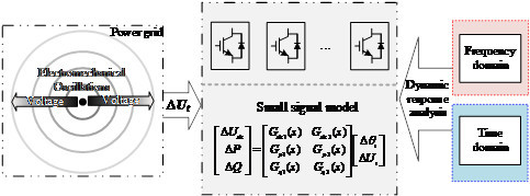
In accordance with Figure 2, the dynamic trajectory of the GVSC DC voltage, active power, and reactive power can be described with voltage amplitude and phase as the basis, as shown in Equation (20). The expressions of the transfer function matrix elements are shown in Appendix A.

$$\left[\begin{array}{c}\Delta U_{dc}\\ \Delta P\\ \Delta Q\end{array}\right]=\left[\begin{array}{cc}{G}_{dc1}\left(s\right)& G_{dc2}\left(s\right)\\ G_{p1}\left(s\right)& G_{p2}\left(s\right)\\ G_{q1}\left(s\right)& G_{q2}\left(s\right)\end{array}\right]\left[\begin{array}{c}\Delta {\theta }_t\\ \Delta U_t\end{array}\right]$$

(20)

When the EO of the power system is determined, i.e., the input of the model is known, the frequency responses of G_p1(s), G_p2(s), G_q1(s), G_q2(s), G_dc1(s), and G_dc2(s) in the electromechanical bandwidth can reflect GVSC response during an EO. Thus, the transfer function matrix is analyzed through the frequency domain method, as shown in Figure 3. However, the time scale of the PLL should be close to the electromagnetic bandwidth [11]. Therefore, the response of the GVSC is mainly affected by G_dc2(s), G_p2(s), and G_q2(s).

The Bode amplitudes of G_dc2(s), G_p2(s), and G_q2(s) according to the parameters in

Table 1. GVSC parameters.

Parameters	Values
Grid voltage	1.01 p.u.
Reference voltage	1.03 p.u.
DC voltage	1.00 p.u.
DC capacitor	0.047 F
Transmission line reactance	0.40 p.u.
Filter inductance	0.32 mH
q-Axis current control loop (kpid, kiid)	0.30, 160
q-Axis current control loop (kpiq, kiiq)	0.30, 160
DC voltage control loop (kpdc, kidc)	3.50, 140
Terminal voltage control loop (kpa, kiac)	1.00, 100

which is used in [12] are shown in Figure 4. For a certain oscillation mode, the DC voltage, active power, and reactive power of the GVSC oscillate in the corresponding mode. Under the same based power, the oscillation amplitude of reactive power should be much larger than that of active power. This phenomenon can be explained through the small signal model shown in Figure 2. The active power forms a closed-loop feedback through Gc(s), which can suppress the response.

The parameters related to G_dc2(s), G_p2(s), and G_q2(s) can be divided into three categories, namely, control parameters, including k_pdc, k_idc, k_pac, k_iac, k_pid, k_iid, k_piq, and k_iiq; operation parameters, including U_ref, X_s, P₀, and U_G0; and DC parameter C. The design of control parameters and DC capacitor needs to consider the time-scale constraints of the cascade control system to ensure the stable operation of the GVSC. Moreover, these parameters do not change with the operating state and network structure. In addition, P₀ is required to be equal to 1 to improve the power factor. Therefore, this study considers the influences of changes in X_s, U_ref, and U_G0 on the dynamics of the GVSC. According to the expressions of G_dc2(s) and G_p2(s), the ASFs of G_dc2(s) and G_p2(s) with respect to U_ref are shown in Figure 5 and Figure 6, respectively. Their values are less than 0 in the electromechanical bandwidth, and thus, the DC voltage and active power of the GVSC weaken as U_ref increases.

Figure 7 shows the MoRSF of G_q2(s) with respect to X_s, U_ref, and U_G0. Overall, they rarely change with the frequency in the electromechanical bandwidth. The MoRSF of G_q2(s) with respect to X_s is maintained at approximately 0.98, which is the largest, followed by that of U_G0, which is 0.25 less than that of X_s; the smallest is U_ref, remaining at approximately 0.2.

The ASFs of X_s, U_ref, and U_G0 are calculated to further analyze the effects of their changes on the reactive power response of the GVSC, as shown in Figure 8. In the electromechanical bandwidth, the ASFs of U_ref and U_G0 are respectively maintained to be greater than 0 at approximately 0.3 and 2.5, respectively. Hence, their increase will enhance the reactive power response of the GSVC during an EO. Although the ASF of X_s increases with incremental frequency, it is always less than 0 in the electromechanical bandwidth. Hence, the increase in X_s will weaken the reactive power response.

In summary, the frequency domain analysis of GVSC in the electromechanical bandwidth shows that the dynamic response of GVSC is mainly expressed by the change of reactive power. The sensitivity of line reactance, grid voltage, and reference voltage to the dynamic response of GVSC decreases in order. As line reactance decreases, the dynamic response of GVSC is enhanced. On the contrary, the decrease of grid voltage and reference voltage weaken the dynamic response of GVSC

5. Simulation and Analysis

This study used the numerical integration method to calculate the time domain trajectory of the DC voltage and AC power of a GVSC during an EO. The power system EO was produced by performing a small disturbance in the IEEE 10-machine power system. The full-power converter-based generation systems in reference [11] were used to analyze GVSCs’ dynamic behavior. The parameters of the GVSC were consistent with those in Table 1. If the network structure and line parameters of the power system were not changed, then the grid strength can be changed by adjusting the transmission line reactance X_l, as shown in Figure 9.

The oscillation component of active power from bus 28 to 29 caused by a small disturbance is shown in Figure 10. This component is used to reflect the power system’s electromechanical behavior. The FT spectrum indicates two oscillation modes in the active power signal, namely, P-1 and P-2. The adaptive local iterative filter decomposition (ALIFD) algorithm was utilized to identify the oscillation’s characteristic parameters (frequency and damping ratio) [28]. As shown in

Table 2. Oscillation parameters of active power in line.

Mode	Frequency (Hz)	Damping Ratio (%)
1	0.6579	6.89
2	1.2651	7.53

, the frequencies of P-1 and P-2 were 0.6579 and 1.2651 Hz, respectively; both values were within the range of the electromechanical bandwidth. The damping ratios of P-1 and P-2 were 6.89% and 7.53%, respectively.

The oscillation component of the DC voltage of a GVSC is shown in Figure 11. Similar to the active power from bus 26 to 27, the DC voltage exhibits a declining trend and comprises two oscillation modes. According to the ALIFD parameter identification results shown in

Table 3. Oscillation parameters of DC voltage.

Mode	Frequency (Hz)	Damping Ratio (%)
1	0.6607	6.73
2	1.2714	7.24

, the low-frequency component in the DC voltage, U_dc-1, had an oscillation frequency of 0.6607 Hz and a damping ratio of 6.73%; these values were similar to those for P-1. The high-frequency component in the DC voltage, U_dc-2, had an oscillation frequency of 1.2714 Hz and a damping ratio of 7.24%; these values were similar to those for P-2.

The oscillation trajectory of the power of the GVSC is shown in Figure 12. The active power and reactive power from the GVSC to the grid comprised two oscillation modes. The oscillation parameters identified by the ALIFD algorithm are shown in

Table 4. Oscillation parameters of AC power.

Signal	Mode	Frequency (Hz)	Damping Ratio (%)
Active power	1	0.6499	6.63
	2	1.2425	7.79
Reactive power	1	0.6513	6.94
	2	1.2688	7.51

. In active power, the oscillation frequency of mode 1 was 0.6499 Hz, and the damping ratio was 6.63%; the oscillation frequency of mode 2 was 1.2425 Hz, and the damping ratio was 7.79%. In the reactive power, the oscillation frequency of mode 1 was 0.6513 Hz, and the damping ratio was 6.94; the oscillation frequency of mode 2 was 1.2688 Hz, and the damping ratio was 7.51. Although the active power and reactive power had frequencies and damping ratios that were similar to those of the power system’s EO, the time domain trajectory denotes that the active power response of the GVSC is much weaker than the reactive power response regardless of the mode (i.e., mode 1 or mode 2).

In the time domain analysis, the instantaneous amplitude was an important indicator to reflect the strength of system response in real-time. For different oscillation signals in the same mode, the instantaneous amplitude was only affected by the initial amplitude (IA). As a result, the response degree of the system can be analyzed by identifying the IA of the oscillating signal. Mode 2 is taken as an example. If the IA of the signal is taken as functions of X_l, U_ref, and U_G0, the partial derivative of the function can directly reflect the influence of parameter changes on GVSC dynamics.

Figure 13 shows the relationship of the deviation in the parameters with the deviations in the IAs of the DC voltage (ΔIA_Udc), active power (IA_P), and reactive power (ΔIA_Q). The ratio of ΔIA_Udc to ΔU_ref, as well as the ratio of ΔIA_P to ΔU_ref, is less than 0. The ratios of ΔIA_Q to ΔU_ref and the ratios of ΔIA_Q to ΔU_G0 were greater than zero, as opposed to the ratio of ΔIA_Q to ΔX_l. Given that ΔX_l, ΔU_ref, and ΔU_G0 have the same unit, the influences of X_l, U_ref, and U_G0 on the reactive power response of the GVSC can also be compared in Figure 13. For the same ΔX_l, ΔU_ref, and ΔU_G0, the variation in reactive power caused by ΔX_l was the largest, followed by that caused by ΔU_G0 and that caused by ΔU_ref. The dynamic response characteristics of GVSC in the time domain were consistent with the results of the frequency domain analysis.

6. Experimental Studies

The GVSC prototype equipment with 5 kW DC power was used to build the power hardware-in-the-loop (PHIL) platform to reflect the response characteristics of the GVSC in the actual grid during the EO, as shown in Figure 14.

The oscillation component of the active power from bus 7 to 9 is shown in Figure 15 In the electromechanical bandwidth, an interarea mode with a frequency and a damping ratio of 0.5312 Hz and 14.96%, respectively, was extracted. Figure 16 shows the oscillation component of the DC voltage and AC power of the GVSC. The active power response of the GVSC was much weaker than its reactive power response. The characteristic parameters of the GVSC’s port variables were extracted by the ALIFD algorithm, as shown in

Table 5. Oscillation parameters of GVSC port variables.

Signal	Frequency (Hz)	Damping Ratio (%)
DC voltage	0.5322	14.33
Active power	0.5267	15.21
Reactive power	0.5338	14.89

. The oscillation frequencies and damping ratios of the DC voltage, active power, and reactive power were 0.5322 Hz and 14.33%, 0.5267 Hz and 15.21%, and 0.5338 Hz and 14.89%, respectively. All of these oscillation characteristic parameters were similar to those in the interarea mode.

Table 6. IA of GVSC response with various parameters.

No.	Xl	Uref	UG0	IAUdc (10−3)	IAP (10−3)	IAQ (10−1)
1	0.10	1.01	1.0	0.521	0.833	0.951
2	0.11	1.01	1.0	0.521	0.833	0.933
3	0.12	1.01	1.0	0.521	0.833	0.917
4	0.10	1.02	1.0	0.508	0.821	0.955
5	0.10	1.03	1.0	0.495	0.797	0.959
6	0.10	1.01	1.01	0.521	0.833	0.960
7	0.10	1.01	1.02	0.521	0.833	0.972

shows the IAs of the DC voltage (IA_Udc), reactive power (IA_P), and active power (IA_Q) under the conditions of seven different sets of parameters. A comparison of Nos. 1, 2, and 3 showed that the increase in X_l made IA_Q increase and left IA_Udc and IA_P unchanged. A comparison of Nos. 1, 4, and 5 indicated that IA_Q increased with an increase in U_ref, whereas IA_P and IA_Udc decreased with an increase in U_ref. A comparison of Nos. 1, 6, and 7 showed that an increase in U_G0 made IA_Q increase and left IA_P and IA_Udc unchanged. When X_l increased from 0.1 to 0.12, the deviation in IA_Q was the largest, 0.034; when U_ref increased from 1.01 to 1.03, the deviation in IA_Q was the smallest, 0.008; when U_G0 increased from 1.0 to1.02, the deviation in IA_Q is 0.021. With the increase of line reactance, the dynamic response of the GVSC under the electromechanical time-scale was enhanced. On the contrary, with the increase of gird voltage and reference voltage, the dynamic behavior of GVSC was weakened.

7. Conclusions

In this study, the DC voltage and AC power of a GVSC were set as the observed signals to investigate the GVSC’s dynamic behavior after a small disturbance in the power system. The dynamic response of the GVSC in the electromechanical bandwidth was analyzed using frequency response and frequency domain sensitivity on the basis of the derived small-signal model. Simulations and experiments conform to the analysis results. The conclusions are as follows.

The time–frequency analysis of the simulation results quantitatively illustrates the correlation between the GVSC’s dynamic response and the electromechanical behavior of the power system from the perspectives of oscillation frequency and damping ratio. Driven by the electromechanical behavior of the power system, the GVSC generates the same mode oscillation as an EO, which can be observed by the DC voltage and AC power of the GVSC, especially the reactive power. Compared with the grid strength and grid voltage, varying reference values of the terminal voltage exert a weak effect on the dynamic behavior of the GVSC during the EO. Although a large grid voltage and a strong grid can enhance the dynamic response of GVSCs, grid strength is sensitive. The dynamic process of GVSC under the electromechanical time scale will be coupled with the dynamic behavior of the system, which may make large-scale renewable penetration threatens the small signal stability of the system. By adding damping control to the GVSC, the small signal stability of the power system with renewable power generation can be improved.

References

- Flourentzou, N.; Agelidis, V.G.; Demetriades, G.D. VSC-based HVDC power transmission systems: An overview. IEEE Trans. Power Electron. 2009, 24, 592–602. [Google Scholar] [CrossRef]
- Zhou, S.; Rong, F.; Yin, Z.; Huang, S.; Zhou, Y. HVDC transmission technology of wind power system with multi-phase PMSG. Energies 2018, 11, 3294. [Google Scholar] [CrossRef] [Green Version]
- Raza, A.; Liu, Y.; Rouzbehi, K.; Jamil, M.; Gilani, S.O.; Dianguo, X.; Williams, B.W. Power dispatch and voltage control in multiterminal HVDC systems: A flexible approach. IEEE Access 2017, 5, 24608–24616. [Google Scholar] [CrossRef] [Green Version]
- Li, Q.; Zhang, Y.; Ji, T.; Lin, X.; Cai, Z. Volt/var control for power grids with connections of large-scale wind farms: A review. IEEE Access 2018, 6, 26675–26692. [Google Scholar] [CrossRef]
- Oprea, S.; Bâra, A.; Preoţescu, D.; Elefterescu, L. Photovoltaic power plants (PV-PP) reliability indicators for improving operation and maintenance activities. A case study of PV-PP Agigea located in Romania. IEEE Access 2019, 7, 39142–39157. [Google Scholar] [CrossRef]
- Gautam, D.; Vittal, V.; Harbour, T. Impact of increased penetration of DFIG–based wind turbine generators on transient and small signal stability of power systems. IEEE Trans. Power Syst. 2009, 24, 1426–1434. [Google Scholar] [CrossRef]
- Shen, P.; Guan, L.; Huang, Z.; Wu, L.; Jiang, Z. Active-current control of large-scale wind turbines for power system transient stability improvement based on perturbation estimation approach. Energies 2018, 11, 1995. [Google Scholar] [CrossRef] [Green Version]
- Kim, H.; Kim, S.; Ko, H. Modeling and control of PMSG-based variable-speed wind turbine. Electr. Power Syst. Res. 2010, 80, 46–52. [Google Scholar] [CrossRef]
- Huang, H.; Mao, C.; Lu, J.; Wang, D. Small-signal modelling and analysis of wind turbine with direct drive permanent magnet synchronous generator connected to power grid. IET Renew. Power Gener. 2012, 6, 48–58. [Google Scholar] [CrossRef]
- Giddani, O.K.; Grain, P.A.; Olimpo, A.; Stephen, L.; Kjetil, U. Small-signal stability analysis of multi-terminal VSC-based DC transmission systems. IEEE Trans. Power Syst. 2012, 27, 1818–1830. [Google Scholar]
- Huang, Y.; Zhai, X.; Hu, J.; Liu, D.; Lin, C. Modeling and stability analysis of VSC internal voltage in DC-link voltage control timescale. IEEE Trans. Power Syst. 2018, 6, 16–28. [Google Scholar] [CrossRef]
- Yuan, H.; Yuan, X.; Hu, J. Modeling of grid-connected VSCs for power system small-signal stability analysis in DC-link voltage control timescale. IEEE Trans. Power Syst. 2017, 32, 3981–3991. [Google Scholar] [CrossRef]
- Amin, M.; Molinas, M. Small-signal stability assessment of power electronics based power systems: A discussion of impedance- and eigenvalue-based methods. IEEE Trans. Ind. Appl. 2017, 53, 5014–5030. [Google Scholar] [CrossRef]
- Raza, M.; Araujo, E.P.; Bellmunt, O.G. Small-signal stability analysis of offshore AC network having multiple VSC-HVDC systems. IEEE Trans. Power Deliv. 2018, 33, 830–839. [Google Scholar] [CrossRef]
- Revel, G.; Leon, A.E.; Alonso, D.M.; Moiola, J.L. Dynamics and stability analysis of a power system with a PMSG-based wind farm performing ancillary services. IEEE Trans. Circuits System I Regul. Pap. 2014, 61, 2182–2193. [Google Scholar] [CrossRef]
- Zhang, L.; Harnefors, L.; Nee, H.P. Modeling and control of VSC-HVDC links connected to island systems. IEEE Trans. Power Syst. 2011, 26, 783–793. [Google Scholar] [CrossRef]
- Slootweg, J.G.; Kling, W.L. The impact of large scale wind power generation on power system. Electr. Power Syst. Res. 2003, 67, 9–20. [Google Scholar] [CrossRef]
- Smith, J.C.; Milligan, M.R.; DeMeo, E.A.; Parsons, B. Utility wind integration and operating impact state of the art. IEEE Trans. Power Syst. 2007, 22, 900–908. [Google Scholar] [CrossRef]
- Quintero, J.; Vittal, V.; Heydt, G.T.; Zhang, H. The impact of increased penetration of converter control-based generators on power system modes of oscillation. IEEE Trans. Power Syst. 2014, 29, 2248–2256. [Google Scholar] [CrossRef]
- Renedo, J.; Cerrada, A.G.; Rouco, L. Active power control strategies for transient stability enhancement of AC/DC grids with VSC-HVDC multi-terminal systems. IEEE Trans. Power Syst. 2016, 31, 4595–4604. [Google Scholar] [CrossRef]
- Renedo, J.; Cerrada, A.G.; Rouco, L. Reactive-power coordination in VSC-HVDC multi-terminal systems for transient stability improvement. IEEE Trans. Power Syst. 2017, 32, 3758–3767. [Google Scholar] [CrossRef]
- Du, W.; Chen, X.; Wang, H.F. Power system electromechanical oscillation modes as affected by dynamic interactions from grid-connected PMSGs for wind power generation. IEEE Trans. Sustain. Energy 2017, 8, 1301–1312. [Google Scholar] [CrossRef]
- Chaudhuri, N.R.; Majumder, R.; Chaudhuri, B.; Jiuping, P. Stability analysis of VSC MTDC grids connected to multimachine AC systems. IEEE Trans. Power Deliv. 2011, 26, 2774–2784. [Google Scholar] [CrossRef]
- Wenyuan, W.; Beddard, A.; Barnes, M.; Marjanovic, O. Analysis of active power control for VSC HVDC. IEEE Trans. Power Deliv. 2014, 29, 1978–1988. [Google Scholar]
- Li, S.; Mike, B.; Robin, P.; Jovica, V.M.; Keith, B.; Manolis, B. The effect of VSC-HVDC control on AC system electromechanical oscillations and DC system dynamics. IEEE Trans. Power Deliv. 2016, 31, 1085–1095. [Google Scholar]
- Huang, Y.; Wang, D. Effect of control-loops interactions on power stability limits of VSC integrated to AC system. IEEE Trans. Power Deliv. 2018, 33, 301–310. [Google Scholar] [CrossRef]
- Karnavas, W.J.; Sanchez, P.J.; Bahill, A.T. Sensitivity analyses of continuous and discrete systems in the time and frequency domains. IEEE Trans. Syst. Man Cybern. 1993, 23, 488–501. [Google Scholar] [CrossRef] [Green Version]
- Yang, D.; Wang, B.; Cai, G.; Wen, J. Oscillation mode analysis for power grids using adaptive local iterative filter decomposition. Int. J. Electr. Power Energy Syst. 2017, 92, 1–13. [Google Scholar] [CrossRef]
Figure 1.
Topology and control system of grid-tied voltage source converter (GVSC).
Figure 2.
Small signal model of the GVSC.
Figure 3.
Frequency domain analysis for GVSC.
Figure 4.
Bode gain diagram of the transfer function matrix.
Figure 5.
Amplitude sensitivity function (ASF) of Gdc2(s) with respect to Uref.
Figure 6.
ASF of Gp2(s) with respect to Uref.
Figure 7.
The magnitude of the relative sensitivity function (MoRSF) of Gq2(s) with respect to operation parameters.
Figure 8.
ASF of Gq2(s) with respect to operation parameters.
Figure 9.
Single-line diagram of the (IEEE) 10-machine power system.
Figure 10.
Time domain trajectory of active power from bus 28 to 29.
Figure 11.
Time domain trajectory of DC voltage of GVSC.
Figure 12.
Time domain trajectory of AC power of GVSC.
Figure 13.
Initial amplitude( IA )deviation curves of (a) GVSC DC voltage, (b) active power, and (c) reactive power.
Figure 14.
(a) Power hardware-in-the-loop (PHIL) platform. (b) Single line diagram of a two-area power system.
Figure 15.
The measured response of tie-line active power.
Figure 16.
Measured response of port variables of GVSC.