Article

An Accurate State of Charge Estimation Method for Lithium Iron Phosphate Battery Using a Combination of an Unscented Kalman Filter and a Particle Filter

Department of Electrical Engineering, Soongsil University, Seoul 06978, Korea
*
Author to whom correspondence should be addressed.
Energies 2020, 13(17), 4536; https://doi.org/10.3390/en13174536
Submission received: 7 August 2020 / Revised: 22 August 2020 / Accepted: 31 August 2020 / Published: 1 September 2020

Abstract

:
An accurate state of charge (SOC) estimation of the battery is one of the most important techniques in battery-based power systems, such as electric vehicles (EVs) and energy storage systems (ESSs). The Kalman filter is a preferred algorithm in estimating the SOC of the battery due to the capability of including the time-varying coefficients in the model and its superior performance in the SOC estimation. However, since its performance highly depends on the measurement noise (MN) and process noise (PN) values, it is difficult to obtain highly accurate estimation results with the battery having a flat plateau OCV (open-circuit voltage) area in the SOC-OCV curve, such as the Lithium iron phosphate battery. In this paper, a new integrated estimation method is proposed by combining an unscented Kalman filter and a particle filter (UKF-PF) to estimate the SOC of the Lithium iron phosphate battery. The equivalent circuit of the battery used is composed of a series resistor and two R-C parallel circuits. Then, it is modeled by a second-order autoregressive exogenous (ARX) model, and the parameters are identified by using the recursive least square (RLS) identification method. The validity of the proposed algorithm is verified by comparing the experimental results obtained with the proposed method and the conventional methods.

Graphical Abstract

1. Introduction

At present, many companies, under the support of governments or organizations, put much effort into developing battery-powered vehicle applications. Lithium is an attractive material for high energy density batteries due to its relatively lower equivalent weight and higher standard potential. It provides much higher power and energy densities in both gravimetric and volumetric terms, which are the most important parameters for applications in portable electronics, such as smartphones, digital cameras, and laptops. Lithium-ion (Li-ion) batteries come in many variations, and the Lithium cobalt oxide (LiCoO2) battery and the Lithium iron phosphate (LiFePO4) battery are popular Li-ion batteries. Despite its lower energy density and lower nominal voltage as compared to cobalt-based Li-ion batteries, the LiFePO4 (LFP) batteries are widely investigated due to their lower cost, superior safety, and greater longevity [1,2,3,4]. Recently, the LFP battery has had a significant growth in the use of energy storage systems (ESS) and electric vehicles (EVs). Therefore, the need for a battery management system, which can accurately estimate the state of charge (SOC) of the battery, is also increasing.
However, unlike the other Li-ion batteries, the LFP battery shows a strong hysteresis phenomenon, which means that the SOC–open-circuit voltage (OCV) relationships during the charge and discharge are quite different [5]. In addition, a flat and long SOC-OCV plateau in between 20% of SOC to 80% of SOC has a significant influence in the accurate estimation of the SOC [6]. Since the SOC of the battery cannot be directly measured by the sensors, it is commonly calculated by the Coulomb counting method using current integration. It simply calculates the remaining capacity by accumulating the charging and discharging currents over time. However, due to the losses and the error of the sensor, it can hardly last long without accumulating errors.
Among various SOC estimation algorithms, the battery model-based approach is the most attractive one. In this method, since the accuracy of the battery model directly affects the SOC estimation accuracy, the battery model needs to be constructed and carefully examined before it is used. Therefore, the battery model should be accurate enough to represent the dynamic behaviors of the battery. In addition, it should be simple enough to establish the state equations and to extract the battery parameters. The most popular one is composed of an OCV indicated by a Direct Current (DC) source and a series resistor connected in series with a parallel branch having a resistor and a capacitor connected in parallel, which is the so-called Randle’s circuit [7]. However, it is already well known that Randle’s model is not good enough to explain all of the reactions taking place inside of the battery. Therefore, a more complex model is often employed for accurate SOC estimation of the battery. In addition, the battery parameter values are critical in estimating the SOC of the battery since the OCV is estimated based on the equivalent circuit model (ECM). There are two different kinds of parameter estimation methods. One is the off-line parameter estimation method [8,9]. Since, however, the battery parameters vary significantly according to the operating conditions, such SOC, temperature, and amplitude of the current, many kinds of different pretests are required to obtain the parameters in different conditions. Since it is extremely time-consuming and labor-intensive work, employing an online parameter estimation algorithm, such as recursive least square (RLS) algorithm with an autoregressive exogenous (ARX) model, is preferred. It is also useful to track the actual changes in parameter values over the life of battery [10,11].
There are several effective methods to estimate the SOC of the battery, such as extended Kalman filters (EKFs), unscented Kalman filters (UKFs), and particle filters (PFs) [11]. The EKF technique is often used for a discrete-time nonlinear dynamic system, such as the SOC estimation of the battery. In this technique, the linearization process is required to approximate the nonlinear system via the Taylor expansion. However, this approximation can introduce large errors in the true posterior mean and covariance of the transformed Gaussian random variables [12]. In [13], the author presents a method for battery SOC estimation using an EKF. In the proposed method, the battery SOC is included as a part of the battery states so that the EKF can automatically compute the dynamic error bounds of the SOC. The UKF can be regarded as a more accessible approach for nonlinear systems than EKFs since it uses a set of carefully chosen sample points and a third-order Taylor expansion. However, the major drawback of these methods is that the process noise and measurement noise, which have a significant influence on the convergence rate and SOC estimation accuracy, need to be obtained based on the trial and error basis. Thus, some kind of adaptive approach is often employed to minimize the effect of these noises.
Unlike the EKF method, the particle filter (PF) works particularly well for nonlinear and robust problems [14]. The particle filter estimates state variables through four steps: initialization, importance sampling, resampling, and normalization. The basic idea of PF is to make predictions through the initial values and state equations of the particles, and the predicted particles are weighted by the likelihood function centered on the measured value. Through the resampling process, the particles with lower weights disappear, and the particles with higher weights multiply. These particles have a uniform weight through normalization, and the process is repeated to estimate the state variables. In PF, the measurement noise standard deviation of the likelihood function is determined by trial and error. The standard deviation value determined at this time does not change. However, the actual measurement noise is time-varying, which limits the estimation performance of the PF. However, in the UKF, the adaptive function can be adapted to time-varying noise by updating the covariance of measurement noise (MN) and process noise (PN). In this case, the MN standard deviation used for the likelihood function of the PF can improve the estimation performance of the PF by using the MN covariance of the UKF.
In this work, the double polarization (DP) model, which can represent the characteristics of a LiFePO4 battery in a more precise way, was used to obtain the accurate SOC estimation results and an ARX model and the recursive least square (RLS) identification method was used for the online identification of the battery parameters to obtained robust SOC estimation results. In the proposed method, an integrated SOC estimator was introduced based on the adaptive UKF and PF. The standard deviation of the likelihood function in the PF was updated by using the covariance of MN in the UKF to improve the convergence time and the accuracy of SOC estimation. The flowchart of the proposed method is shown in Figure 1.
This paper is organized as follows. The battery cell model using a second-order ECM and ARX model is established in Section 2. The RLS parameter identification algorithm by the ARX model is discussed in Section 3. In Section 4, the proposed algorithm is introduced based on a UKF and a PF. The reliable and robust performance of the proposed algorithm is verified through experiments in Section 5. Finally, the conclusions of this research and the future plan are provided in Section 6.

2. Battery Modeling

2.1. Equivalent Circuit Model (ECM)

For accurate SOC estimation, it is important to use an accurate ECM for the battery, especially for the battery, such as LiFePO4, which has a flat plateau on the OCV-SOC curve. Various kinds of battery models have been developed to represent the static and dynamic characteristics of the battery. Among them, the ECMs composed of a voltage resource, resistors, and capacitors are widely used. Based on the combination of resistors and capacitors, the ECMs are classified into several kinds, such as the Rint Battery model [15], Thevenin model [16], improved Thevenin model named the double polarization (DP) model [17] and, etc. Generally, the Thevenin models consist of a voltage resource, an ohmic resistor, and several RC networks. Typically, the component count of the ECM tends to be increased to precisely describe the dynamic behavior of the battery. Therefore, the SOC estimation accuracy can also be improved if a higher-order ECM is used. However, since the computational burden of the SOC estimation is proportional to the complexity of the model, it is desirable to select a suitable battery model to achieve an accurate SOC estimation with a reasonable amount of computation. In [7,18], the performances of the seven representative ECMs have been evaluated, and it has been proven that the DP model is optimal among them in terms of optimal performance [7,18].
In this research, the DP model consisting of an OCV-UOC, an Ohmic resistance Ri, and two RC networks, was selected as an ECM of the LFP battery, as shown in Figure 2.
The charge transfer effect causing a first voltage drop UP on the electrode potential is presented by the charge transfer resistance RP and the double layer capacitance CP with a short time constant. The diffusion effect causing a second voltage drop UD on the electrode potential is presented by RD and CD with a long time constant. The corresponding relationship between UOC and SOC is determined through a SOC-OCV test described in [19]. The electrical behavior of the LFP with the DP model, shown in Figure 2, can be expressed as Equation (1):
U ˙ P / ( R P × C P ) + I b / C P U ˙ D = U D / ( R D × C D ) + I b / C D U b   =   U OC     I b R i     U P     U D

2.2. Second-Order Autoregressive Exogenous (ARX) Model for Parameter Identification

As already well known, the parameters of the ECM of the battery vary depending on the SOC, temperature, and the amplitude of the current applied to the battery [20]. Therefore, to obtain the accurate SOC estimation results, the parameter values in the ECM should be updated at each condition. In the case of the off-line method, the parameter variations of the battery at different conditions are measured by the extensive pretests and used in the form of the lookup table. However, it is a time consuming and labor-intensive work, which increases the cost of the system [20].
The autoregressive exogenous (ARX) model is widely used as a system identification tool in many researches since their optimal predictors are always stable [21]. A practical equation to determine the next output value with previous input values of the 2nd-order ARX model with zero mean white noise e(k) is given as Equation (2).
y ( k )   =   a 1 y ( k     1 )     a 2 y ( k     2 )   +   b 0 u ( k )   +   b 1 u ( k     1 )   +   b 2 u ( k     2 )   +   e ( k )
where y(k) and u(k) indicates the system output and input, respectively. A more compact form of Equation (2) can be obtained as the linear regression.
y ( k )   =   ψ T ( k )   ϑ ( k     1 )   +   e ( k )
In Equation (3), ϑ(k − 1) is the coefficient vector, ψ(k) is the input vector, and e(k) is the error between the measured and estimated values. The coefficient vector and the input vector can be represented as follows:
ϑ ( k )   =   [   a 1 ;   a 2 ;   b 0 ;   b 1 ;   b 2 ] T   ψ ( k )   =   [ y ( k     1 ) ,   y ( k     2 ) ,   u ( k ) ,   u ( k     1 ) ,   u ( k     2 ) ] T  
On the other hand, according to the electrical behavior of the ECM of the battery expressed in Equation (1), the transfer function given by the Laplace equation for the battery impedance can be deduced in the s domain as:
G ( s )   =   U I m p ( s ) I b ( s )   =   U b ( s )     U O C ( s ) I b ( s )   =   R i   + R P 1   +   s R P C P   +   R D 1   +   s R D C D
Equation (5) can be rewritten as a simple form by Equation (6).
G ( s )   =   K 1 s 2 +   K 5 K 2 s +   K 4 K 2 s 2 + K 3 K 2 s + 1 K 2
where:
K 1   =   R i K 2   =   R P C P R D C D K 3   =   R P C P   +   R D C D K 4   =   R i   +   R P   +   R D K 5   =   R i R P C P   +   R i R D C D   +   R P R D C D   +   R D R P C P
The basic forward Euler transformation method, a simple yet accurate approximation with a small step interval Ts, is employed in the computational process of discretization. By substituting s in Equation (6) by   ( 1     z 1 ) / ( T s z 1 ) , a discrete form of the transfer function can be obtained as Equation (8).
G ( z )   =   b 0   +   b 1 z 1 +   b 2 z 2 1     a 1 z 1     a 2 z 2 a 1   =   2     K 3 K 2 T 2 a 2   =   K 3   1 K 2 T 2   1 b 0   =   K 1 b 1   =   2 K 1     K 5 K 2 T 2 b 2   =   K 4     K 5 K 2 T 2     2 K 2
Hence, the differential equation indicating the time-domain relationship between input and output can be represented as Equation (9):
U b ( k )     U OC ( k )   =     a 1 ( U b ( k     1 )     U OC ( k     1 ) )     a 2 ( U b ( k     2 )     U OC ( k     2 ) )   +   b 0 I b ( k )   +   b 1 I b ( k     1 )   +   b 2 I b ( k     2 )
The above function indicates the 2nd-order ARX model of Equation (2) for the battery ECM in Figure 2, and the parameters of the system can be extracted by using a parameter identification method, such as the RLS method.

3. Dynamic Parameter Identification Algorithm Using the Autoregressive Exogenous Model

The dynamic parameters of an LFP battery are identified by the RLS algorithm based on the established ARX model. The operating principle of the parameter identification algorithm, such as RLS, is basically to compute the parameter update at a time index k by adding a correction term to the previous parameter at a time index k − 1 once the new information is available [22]. Considering the dynamic battery parameters and the time-domain relationship between input and output in Equation (9), the system identification using the RLS algorithm can be summarized as follows [23]:
System output:
y ( k ) = ψ T ( k ) ϑ ^ ( k 1 )
Prediction error:
ε ( k ) = U b ( k ) U O C ( k ) ψ T ( k ) 1
Updated gain:
K ( k )   =   P ( k     1 ) ψ T ( k ) λ   +   ψ T ( k ) P   ( k     1 ) ψ ( k )  
Covariance matrix:
P ( k )   =   P ( k     1 )     K ( k ) ψ T ( k )   P ( k     1 ) λ ( k )
Estimated parameter:
ϑ ^ ( k ) = ϑ ^ ( k 1 ) + K ( k ) ε ( k )
Parameters and input vector:
ϑ ( k )   =   [   a 1 ;   a 2 ;   b 0 ;   b 1 ;   b 2 ]
ψ ( k )   =   [ ( U b ( k     1 )     U O C ( k     1 ) ) ,     ( U b ( k     2 )     U O C ( k     2 ) ) ,   I b ( k ) ,   I b ( k     1 ) ,   I b ( k     2 ) ] T
where ψ(k) is the input vector obtained from input data values including the terminal voltage of the battery Ub(k − 1) and Ub(k − 2) at the time index k − 1 and k − 2, UOC(k − 1) and UOC(k − 2) are the open circuit voltages at time index k − 1 and k − 2, Ib(k), Ib(k − 1) and Ib(k − 2) are the battery currents at the time index k, k − 1 and k −2, respectively. ϑ ^ ( k ) is the coefficient vector, which needs to be identified. λ(k) (0 < λ < 1) is a forgetting factor which can be used to give greater weight to the recent data than the old one.
After the estimated parameter vector ϑ ^ ( k ) is identified, the parameters of the battery model at each time index can be determined by Equation (16).
R i   =   b 0 R P C P R D C D   =   T 2 1     a 1     a 2 R P C P   +   R D C D   =   2     a 1 1     a 1     a 2 R i   +   R P   +   R D   =   b 1   +   b 2 1     a 1     a 2 R i R P C P   +   R i R D C D   +   R P R D C D   +   R D R P C P   =   2 b 0     b 1 1   a 1     a 2 T s

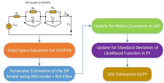
4. Proposed SOC Estimation Algorithm Using a Combination of UKF and PF

The general mathematical function of the battery model, including the state equation and the observation equation of the discrete system, can be expressed by Equation (17).
x k   =   A k x k 1   +   B k u k   +   w k y k   =   C k x k   +   D k u k   +   v k
where xk represents the system state at time index k, uk stands for the input of the system, including battery current, yk is the observed output which indicates battery terminal voltage, wk and vk are independent process noise and measurement noise with covariance matrixes Qk and Rk, respectively. Ak and Bk are state matrixes, and Ck and Dk are observed matrixes.
The state–space model of the battery can be represented in the form of the discrete-time equation, as shown in Equation (18), according to the electrical behavior of the ECM depicted in Figure 2.
x k   = [ U P , k U D , k S O C k ]   =   [ 1 T s / ( R P   C P ) 0 0 0 1 T s / ( R D C D ) 0 0 0 1 ] × [ U P , k 1 U D , k 1 S O C k 1 ] + [ T s / C P T s / C D η I   C n ] × [ I b , k ] +   w k U b , k   =   U O C , k ( S O C k )     I b , k R i     U P , k     U D , k   +   v k
where ηI and Cn are the columbic efficiency and actual capacity of the battery cell, respectively.

4.1. Unscented Kalman Filter Based SOC Estimation

The UKF based SOC estimation is well known, and it can be summarized as follows [12,24]:
1.
Determination of Scaling and Weights:
Primary, secondary, and scaling parameters:
α, β, κ (default)
Length of state vector: n
Scaling parameter:
λ   =   α 2 ( n   +   κ )   +   n
Weight vector:
W 0 m   =   λ / ( n   +   λ )
W 0 c   =   λ / ( n   +   λ )   +   1     α 2 + β
W i m   =   W i c   =   1 / [ 2 ( n   +   λ ) ] ;   I   =   1 , 2 , 2 n
2.
Initialization:
x ¯ 0 = E ( x 0 ) P 0 = E [ ( x 0 x ¯ 0 ) ( x 0 x ¯ 0 ) T ]
3.
Generation of the Sigma-point:
Error covariance matrix square root:
P k 1   =   c h o l   ( P k 1 )
Sigma-point:
.  
4.
Prediction transformation:
State update:
χ ^ k | k 1 i = A k x ^ k 1 i + B k u k + w k ; i = 0 , 1 , 2 2 n
Mean of the predicted state:
x ^ k | k 1 = i 2 n W i m χ ^ k | k 1 i
Covariance matrix of the predicted state:
P k | k 1 = Q k + i 2 n W i c χ ^ k | k 1 i x ^ k | k 1 χ ^ k | k 1 i x ^ k | k 1 T
5.
Observation transformation
Propagation of sigma-point through observation:
ψ k | k 1 i = C k x ^ k i + D k u k + v k
Update the output:
y ^ k | k 1 = i 2 n W i m ψ ^ k | k 1 i
Covariance matrix of the predicted output:
P x y y = R k + i 2 n W i c ψ k | k 1 i y ^ k | k 1 ψ k | k 1 i y ^ k | k 1 T
Covariance matrix of the predicted state and output:
P x x y = i 2 n W i c χ k | k 1 i x ^ k | k 1 χ k | k 1 i x ^ k | k 1 T
6.
Measurement update
Kalman gain:
K k   =   P k xy [ P k yy ] 1
State estimation measurement update:
x ^ k = x ^ k | k 1 + K k ( y k y ^ k | k 1 )
Error covariance measurement update:
P k   =   P k | k 1   +   K k P k yy K k T

4.2. Particle Filter Based SOC Estimation

The particle filter method assumes that there are many possible predictions, and each of them has its own weight or probability [25]. The state–space variables are estimated by PF through a probability distribution p(xk|yk) that provides the probabilities of possible values of the true state. The step-by-step process for the PF can be expressed as follows [25,26,27]:
1.
Initialization: Randomly draw N initial particles for SOC.
Draw particles x0i~p(x0); i = 1,2,…N.
2.
Sampling and weight calculation: From the distribution, the particles are sampled and updated with new observation information, and then a new sample is obtained.
Likelihood calculation:
p ( y k | x k i )   =   1 2 π R k e x p [ 1 2 ( y k   C k x k i   +   D k u k   +   v k ) 2 / R k ]
Assigning particle a weight:
ω ^ k i = ω k 1 i p ( y k | x k i )
Calculation of the Distribution:
p ( x k | y k 1 i = 1 N ω k 1 i ( A k 1 x ^ k i + B k 1 u k + w k 1 )
Normalization of the weight:
ω k i   =   ω ^ k i / i = 1 N ω ^ k i
3.
Resampling:
Resampling when effective sample size Neff is under the threshold:
N e f f   =   1 / i = 1 N ( ω k i ) 2
Replacing current set by a new one:
ω ˜ k i = 1 / N
4.
State prediction:
x ˜ k = i = 1 N ω ˜ k i x ˜ k i

4.3. Combined SOC Estimation Method by Using UKF and PF

In this paper, a combined SOC estimation method using UKF and PF is proposed. The PF is used for online SOC estimation based on the priori parameter information from ARX-RLS and the OCV information from UKF. In UKF, the PN and MN are assumed to be independent, and the performance of the combined UKF-PF relies on it heavily. When the PN and MN are constant values, the estimation accuracy is limited since the PN and MN are actually varying values. Therefore, the noise covariance needs to be computed at each time of sampling by the following equations [28]:
F k   =   j = k q + 1 k e j e j T q
Q k + 1   =   K k F k K k T
R k + 1 = F k + i 2 n W i c ψ k | k 1 i y ^ k | k 1 ψ k | k 1 i y ^ k | k 1 T
where e and q are the residual error in the measured output and the window size for covariance matching, respectively. Fk represents the covariance approximation of the voltage residual at step j.
The flowchart of the proposed method is shown in Figure 3. The likelihood calculation shown in Equation (35) is quite important in the proposed method because the values for PN and MN for the UKF are calculated at every step, and the updated values are provided to calculate the likelihood of the PF. Here, Rk is the covariance of the measurement noise vk. It affects assigning particles a weight. Since the likelihood of the PF is recalculated every time in the proposed method, the estimation performance can be further improved.

5. Experimental Results and Verification

5.1. Battery Test Bench

The experimental data, such as battery current and voltage, were measured through an established experimental setup in which a Headway 38120S 10Ah LiFePO4 battery was connected to a bipolar DC power supply (NF BP4610). A program composed by LabView (National Instruments, Austin, Texas, USA) was used to control the power supply to regulate the battery current as required. The measured voltage and current data of the cell were recorded in the host computer through the data acquisition board (DAQ 9125, National Instruments, Austin, Texas, USA). The specification of the LiFePO4 battery is shown in Table 1, and the experimental setup is shown in Figure 4.

5.2. Experimental Results and Discussions

To verify the performance of the proposed UKF-PF algorithm, the Urban Dynamometer Driving Schedule (UDDS) was applied to a fully charged battery cell, as shown in Figure 5a [29]. The Constant Current – Constant Voltage (CC-CV) charge method was used to charge the battery up to 100% SOC. The UDDS profile is designed in a way that the battery cell SOC decreases from 100% SOC to 20% SOC, which is the typical operation range of the battery. The Ah counting method by integrating the battery current was used to calculate the reference SOC since quite accurate results can be obtained with the method when the time duration of the experiment is less than a few hours.
At the beginning of the experiment, no load was applied to the battery for 900 s to see the SOC estimation performance of the proposed method during the rest. Then the battery was discharged with the current profile extracted from the UDDS and the 0.5 C rate constant current until the SOC reached 20%. At the first UDDS cycle, the regenerative braking was not applied so as not to exceed the maximum charge voltage of the LFP battery. The total experiment time was 10,700 sec, as shown in Figure 5a. The results in Figure 5b show the good agreement between the measured and the estimated terminal voltages of the battery by the proposed UKF-PF method. Figure 5c shows the SOC estimation results by the proposed method and Ah counting method. Here, 92% SOC was given as an initial value for the test. As shown in Figure 5c, it took 60 s to reach the reference SOC value by the proposed method. The root mean square error (RMSE) of the SOC estimation was 0.769%, while the maximum error was 1%. To compare the performance of the SOC estimation with the proposed method and the other conventional methods, UKF and Adaptive Unscented Kalman Filter (AUKF) algorithms were also used to estimate the SOC with the measured current and voltage waveforms, shown in Figure 5 and Figure 6 which show the experimental results obtained with the proposed UKF-PF method, UKF and AUKF methods.
Figure 6a shows the SOC estimation results by UKF, AUKF, and UKF-PF. The SOC estimation error of each method as compared to the reference value by the Ah counting method is shown in Figure 6b. It is clear that the proposed method showed the shortest convergence time in comparison with the other methods. The maximum SOC estimation error of the proposed UKF-PF method was around 1%, while that of UKF and AUKF was 2.5% and 1.6%, respectively. Table 2 shows the RMSE of the SOC estimation by UKF, AUKF, and proposed UKF-PF method.

6. Conclusions

In this research, an accurate SOC estimation method using a combination of a UKF and a PF suitable for LiFePO4 Battery was proposed, and its validity and feasibility were proven by the experiments. In the proposed UKF-PF method, the DP model was used to represent the characteristics of the battery better. The parameters of the battery were identified by using an ARX model and the RLS algorithm, and it was supplied to the combined UKF-PF algorithm for the robust SOC estimation. The main idea of the proposed method is to update the standard deviation of the likelihood function in the PF by using the covariance of MN in the UKF, thereby improving the convergence time and the accuracy of SOC estimation. In results, the accuracy of the SOC estimation can be further improved to have less than 1% error in terms of RMSE and MAE. The proposed algorithm can be widely employed to provide a reliable SOC estimation for the LFP battery systems, such as electric vehicles and energy storage systems.

Author Contributions

T.-T.N. wrote the manuscript and designed the algorithm of proposed method; A.B.K. analyzed the algorithm of the proposed method; Y.K. helped in preparing the final manuscript.; W.C. reviewed the manuscript and supervised the research. All authors have read and agreed to the published version of the manuscript.

Funding

This research received no external funding.

Acknowledgments

This research was supported by the R&D program for new energy industry through Chungnam Center for Creative Economy and Innovation(CCCEI) funded by Local Government of Chungchengnamdo.

Conflicts of Interest

The authors declare no conflict of interest.

References

  1. Zaghib, K.; Striebel, K.; Guerfi, A.; Shim, J.; Armand, M.; Gauthier, M. LiFePO4/polymer/natural graphite: Low cost Li-ion batteries. Electrochim. Acta 2004, 50, 263–270. [Google Scholar] [CrossRef]
  2. Mi, C.; Cao, G.; Zhao, X. Low-cost, one-step process for synthesis of carbon coated LiFePO4 cathode. Mater. Lett. 2005, 59, 127–130. [Google Scholar] [CrossRef]
  3. Striebel, K.; Shim, J.; Sierra, A.; Yang, H.; Song, X.; Kostecki, R.; McCarthy, K. The development of low cost LiFePO4-based high power lithium-ion batteries. J. Power Sources 2005, 146, 33–38. [Google Scholar] [CrossRef] [Green Version]
  4. Zheng, Y.; Ouyang, M.; Lu, L.; Li, J.; Han, X.; Xu, L.; Ma, H.; Dollmeyer, T.A.; Freyermuth, V. Cell state-of-charge inconsistency estimation for LiFePO4 battery pack in hybrid electric vehicles using mean-difference model. Appl. Energy 2013, 111, 571–580. [Google Scholar] [CrossRef]
  5. Barai, A.; Widanage, W.D.; Marco, J.; Mcgordon, A.; Jennings, P. A study of the open circuit voltage characterization technique and hysteresis assessment of lithium-ion cells. J. Power Sources 2015, 295, 99–107. [Google Scholar] [CrossRef]
  6. Dong, G.; Wei, J.; Zhang, C.; Chen, Z. Online state of charge estimation and open circuit voltage hysteresis modeling of LiFePO4 battery using invariant imbedding method. Appl. Energy 2016, 162, 163–171. [Google Scholar] [CrossRef]
  7. He, H.; Xiong, R.; Guo, H.; Li, S. Comparison study on the battery models used for the energy management of batteries in electric vehicles. Energy Convers. Manag. 2012, 64, 113–121. [Google Scholar] [CrossRef]
  8. Waag, W.; Käbitz, S.; Sauer, D.U. Experimental investigation of the lithium-ion battery impedance characteristic at various conditions and aging states and its influence on the application. Appl. Energy 2013, 102, 885–897. [Google Scholar] [CrossRef]
  9. Shuo, T.; Munan, H.; Minggao, O. An Experimental Study and Nonlinear Modeling of Discharge Behavior of Valve-Regulated Lead Acid Batteries. IEEE Trans. Energy Convers. 2009, 24, 452–458. [Google Scholar] [CrossRef]
  10. Xiong, R.; Sun, F.; He, H.; Nguyen, T.D. A data-driven adaptive state of charge and power capability joint estimator of lithium-ion polymer battery used in electric vehicles. Energy 2013, 63, 295–308. [Google Scholar] [CrossRef]
  11. Hu, X.; Li, S.; Peng, H. A comparative study of equivalent circuit models for Li-ion batteries. J. Power Sources 2012, 198, 359–367. [Google Scholar] [CrossRef]
  12. Wan, E.A.; van der Merwe, R. The unscented Kalman filter for nonlinear estimation. In Proceedings of the IEEE 2000 Adaptive Systems for Signal Processing, Communications, and Control Symposium (Cat. No.00EX373), Lake Louise, AB, Canada, 4 October 2000; pp. 153–158. [Google Scholar]
  13. Plett, G.L. Extended Kalman filtering for battery management systems of LiPB-based HEV battery packs—Part 2. Modeling and identification. J. Power Sources 2004, 134, 262–276. [Google Scholar] [CrossRef]
  14. Wang, Y.; Zhang, C.; Chen, Z. A method for state-of-charge estimation of LiFePO4 batteries at dynamic currents and temperatures using particle filter. J. Power Sources 2015, 279, 306–311. [Google Scholar] [CrossRef]
  15. Chan, H.L. A new battery model for use with battery energy storage systems and electric vehicles power systems. In Proceedings of the IEEE Symposium on Power Engineering Society Winter Meeting, Singapore, 23–27 January 2000; Volume 1, pp. 470–475. [Google Scholar]
  16. Ziyad, M.; Margaret, A.; William, A. A mathematical model for lead-acid batteries. IEEE Trans. Energy Convers. 1992, 7, 93–98. [Google Scholar]
  17. Hongwen, H.; Rui, X.; Xiaowei, Z.; Fenchun, S.; Jinxin, F. State-ofcharge estimation of the lithium-ion battery using an adaptive extended Kalman filter based on an improved Thevenin model. IEEE Trans. Veh. Technol. 2011, 60, 1461–1469. [Google Scholar] [CrossRef]
  18. He, H.; Xiong, R.; Fan, J. Evaluation of Lithium-Ion Battery Equivalent Circuit Models for State of Charge Estimation by an Experimental Approach. Energies 2011, 4, 582–598. [Google Scholar] [CrossRef]
  19. Roscher, M.A.; Sauer, D.U. Dynamic electric behavior and open-circuit-voltage modeling of LiFePO4-based lithium ion secondary batteries. J. Power Sources 2011, 196, 331–336. [Google Scholar] [CrossRef]
  20. Duong, V.H.; Tran, N.T.; Choi, W.; Kim, D. State Estimation Technique for VRLA Batteries for Automotive Applications. J. Power Electron. 2016, 16, 238–248. [Google Scholar] [CrossRef] [Green Version]
  21. Keesman, K.J. System Identification—An Introduction; Springer: London, UK, 2011; pp. 1–13. [Google Scholar]
  22. Jiang, J.; Zhang, Y. A revisit to block and recursive least squares for parameter estimation. Comput. Electr. Eng. 2004, 30, 403–416. [Google Scholar] [CrossRef]
  23. Tran, N.; Khan, A.B.; Choi, W. State of Charge and State of Health Estimation of AGM VRLA Batteries by Employing a Dual Extended Kalman Filter and an ARX Model for Online Parameter Estimation. Energies 2017, 10, 137. [Google Scholar] [CrossRef] [Green Version]
  24. Tian, Y.; Xia, B.Z.; Sun, W. A modified model based state of charge estimation of power lithium-ion batteries using unscented Kalman filter. J. Power Sources 2014, 270, 619–626. [Google Scholar] [CrossRef]
  25. Walker, E.; Rayman, S.; White, R.E. Comparison of a particle filter and other state estimation methods for prognostics of lithium-ion batteries. J. Power Source 2015, 287, 1–12. [Google Scholar] [CrossRef] [Green Version]
  26. Arulampalam, M.S.; Maskell, S.; Gordon, N.; Clapp, T. A tutorial on particle filters for online nonlinear/non-Gaussian Bayesian tracking. IEEE Trans. Signal Process. 2002, 50, 174–188. [Google Scholar] [CrossRef] [Green Version]
  27. Miao, Q.; Xie, L.; Cui, H.; Liang, W.; Pecht, M. Remaining useful life prediction of lithium-ion battery with unscented particle filter technique. Microelectron. Reliab. 2013, 53, 805–810. [Google Scholar] [CrossRef]
  28. Guo, X.; Kang, L.; Yao, Y.; Huang, Z.; Li, W. Joint Estimation of the Electric Vehicle Power Battery State of Charge Based on the Least Squares Method and the Kalman Filter Algorithm. Energies 2016, 9, 100. [Google Scholar] [CrossRef]
  29. Kim, S.; Choi, W. Selection Criteria for Supercapacitors Based on Performance Evaluations. J. Power Electron. 2012, 12, 223–231. [Google Scholar] [CrossRef] [Green Version]
Figure 1. Proposed method block diagram for LiFePO4 (LPF) Battery.
Energies 13 04536 g001
Figure 2. LiFePO4 (LFP) battery cell equivalent circuit model.
Energies 13 04536 g002
Figure 3. Flowchart of the proposed estimation algorithm.
Energies 13 04536 g003
Figure 4. Experimental setup: (a) Block diagram; (b) Picture.
Energies 13 04536 g004
Figure 5. Experimental results: (a) Urban Dynamometer Driving Schedule (UDDS) current profile applied to the LiFePO4 battery; (b) Measured and estimated voltage of the battery; (c) State of charge (SOC) estimation result with the proposed method and Ah counting method.
Energies 13 04536 g005
Figure 6. SOC estimation results with unscented Kalman filter (UKF), Adaptive Unscented Kalman Filter(AUKF), and the proposed UKF- particle filter (PF) method: (a) SOC estimation results of the different methods; (b) SOC estimation error.
Energies 13 04536 g006
Table 1. Specification of a Headway 38120S 10 Ah LiFePO4 battery.
Model38120S
Chemical CompositionLiFePO4
Nominal Capacity10 Ah
Maximum Charge Voltage3.65 V
Nominal Voltage3.2 V
Cut-off Voltage2.0 V
Charge MethodCC-CV
Standard Charge Current5 A
30 A Max
Max. Discharge Current10 A recommended,
30 A (Max. continuous discharge rate),
100 Amp (<30 s)
Operation TemperatureCharge: 0–45 °C (32–113 °F)
Discharge: −20–65 °C (−4–149 °F)
Cycle Performance>2000 (80% of initial capacity at 0.2 C rate, IEC standard)
Table 2. Comparison of performances of the different estimation methods.
MethodProposedUKFAUKF
Root mean square error, RMSE (%)0.7691.8561.013
Maximum absolute error, MAE (%)0.8232.4781.228

