Integrated Approach Based on Dual Extended Kalman Filter and Multivariate Autoregressive Model for Predicting Battery Capacity Using Health Indicator and SOC/SOH

Abstract

To enhance the efficiency of an energy storage system, it is important to predict and estimate the battery state, including the state of charge (SOC) and state of health (SOH). In general, the statistical approaches for predicting the battery state depend on historical data measured via experiments. The statistical methods based on experimental data may not be suitable for practical applications. After reviewing the various methodologies for predicting the battery capacity without measured data, it is found that a joint estimator that estimates the SOC and SOH is needed to compensate for the data shortage. Therefore, this study proposes an integrated model in which the dual extended Kalman filter (DEKF) and autoregressive (AR) model are combined for predicting the SOH via a statistical model in cases where the amount of measured data is insufficient. The DEKF is advantageous for estimating the battery state in real-time and the AR model performs better for predicting the battery state using previous data. Because the DEKF has limited performance for capacity estimation, the multivariate AR model is employed and a health indicator is used to enhance the performance of the prediction model. The results of the multivariate AR model are significantly better than those obtained using a single variable. The mean absolute percentage errors are 1.45% and 0.5183%, respectively.

1. Introduction

Due to the Paris Agreement for preventing catastrophic climate change, the current energy system requires a rapid global shift toward decarbonization in all sectors, such as industry, transportation, and residential and commercial buildings, through the use of renewable energy [1]. The generation of renewable energy must be increased to achieve decarbonization of power and energy systems. Because renewable energy resources have intermittent characteristics, an energy storage system (ESS) is essential for the transition to a sustainable energy system with flexibility and reliability [2]. Among different types of battery, the Lithium-ion battery is effective for high power and high energy density applications and is also widely used from small-to-large scale electronics, electric vehicles, and utility-scale storages [3].

In the global market, the installation of ESSs is expected to increase exponentially, from 9 GW/17 GWh deployed as of 2018 to 1095 GW/2850 GWh expected by 2040 [4]. Studies have indicated that the ability to store and release electricity nearly instantaneously offers multiple benefits in the power system not only for the integration of diverse renewable energy sources but also for grid reliability [5].

To enhance grid efficiency, it is important to consider both the battery cost and the performance of the ESS over its lifespan [6]. The cost of battery packs is decreasing by an average of 13% per year and is expected to reach $156/kWh in 2019 and $100/kWh in 2023 [7]. Because improvements in battery performance can reduce operation and management costs, the importance of the battery management system (BMS) is gradually increasing to manage and monitor the battery state more efficiently. Accurate estimation and prediction of the state of charge (SOC) and the state of health (SOH) can ensure the BMS prolong the cycle life of energy management and reduce the utilization cost for replacing the battery [8].

The SOC represents the remaining capacity that is compared with the stored capacity [9]. The SOC varies between 0% to 100%, which corresponds to the fully discharged and charged state, respectively. However, if the battery is aged, the maximum value of the SOC decreases because of the capacity degradation. When the capacity is reduced to 80% of the initial value, the SOC region of the battery is reduced by 20%. Thus, accurate capacity estimation is required for the efficient and safe operation of the battery [10]. Research on estimating the SOC and SOH, according to the variability of the battery characteristics, is crucial for developing an advanced BMS. Among the estimation strategies, the Kalman filter is advantageous in the sense that it has a very flexible coordinator to handle battery characteristic changes [8,10].

2. Literature Review

The SOH is the ratio of the characterization parameters (e.g., capacity and internal resistance). The remaining useful life (RUL) is the number of available cycles from the SOH to the failure threshold. Among research studies regarding battery, it is a necessity for efficient utilization to identify the aging mechanism and predict the capacity loss based on SOH, according to the different perspectives [11,12].

From an economic viewpoint, because the battery wear cost can be calculated according to the achievable cycle count, depth of discharge, battery size, and round-trip efficiency [13], the SOH can be a reference to determine the battery replacement cost and economic utilization cost for maximizing the profitability [14,15,16]. From a technical perspective, the battery cycle life and SOH can be utilized to optimize the energy management strategy by determining the threshold for energy capability [17]. In the long term, SOH management improves the lifecycle by assessing the impact of battery aging using a health indicator (HI), which tracks the degradation of batteries [17].

In recent studies, estimation methods of the battery capacity have employed the correlation between the characterization parameters and aging. This seems to be an important issue that the estimation method for the HI should be selected properly to reflect the nonlinear pattern of degradation. The integrated HI is defined in the aging model by incorporating a certain period of capacity and resistance. Xiong et al. [18] investigated the correlation between the partial charge capacity obtained in a certain region of the voltage and the capacity for extracting the effective HI in the charging mode. A linear aging model was constructed using the moving-window-based method considering the HI. Zheng et al. [19] utilized the HI to determine the optimal charge region of the fixed voltage window and proposed an online capacity estimation method that incorporates both the discrete Arrhenius aging model and extended Kalman filter. Liu et al. [20] proposed a relevance vector machine using the optimized HI to enhance the accuracy and stability of RUL prediction. Zhou et al. [21] optimized the HI considering the different times of voltage drops in the discharge curve and used the Box-Cox transformation to stabilize the variance. Even though these methods are widely used for estimating the SOH because the capacity is highly dependent on the charge/discharge region, the HI extraction is limited to the charge/discharge region. If the battery voltage does not reach a certain region, the HI cannot be updated and the prediction performance is unreliable. Therefore, aging characterization parameters based on real-time methods are needed to estimate the SOH accurately.

To select the appropriate HI in real-time, resistance is the most influential candidate for reflecting the aging condition of the battery. The resistance is related to the solid-electrolyte interphase (SEI) layer in the physicochemical mechanism of the battery. One of the most influential factors affecting the capacity loss with aging is the SEI layer growth [22]. According to cell size, capacity, cell design, and types of active material in the battery, thermal abuse tolerance of the battery can be varied from the SEI formation [23]. Even though it has a strong relationship with the capacity loss, it is difficult to identify the multi-physical behavior and thermodynamics of the SEI layer in real-time applications because of the model’s complexity and a large number of parameters [24]. The SEI growth for the prediction of the SOH can be simplified by using electrochemical impedance spectroscopy (EIS) and an equivalent circuit model (ECM). The resistance of the SEI layer can be extracted from the high-frequency region of the EIS results and the parameters from EIS can be applied to the ECM [25]. This method has the advantage of quickly extracting the parameters to be implemented in the BMS board [26]. However, it is too complex to conduct computations for fitting a model. Additionally, the EIS is difficult to apply for real-time estimators and applications because it requires the high cost for the experiment [27].

Due to this limitation, the method for estimating the SOH in real-time applications needs to define the relationship between the internal resistance based on the direct-current signal and the capacity. Pan et al. [28] proposed an online SOH estimation method using machine learning and the ECM parameters, such as the enlarged ohmic and polarized internal resistances. Because these parameters are intuitive values and are flexible for different types of dynamic load profiles, they can be measured by an online parameter identification algorithm. However, the machine learning method is difficult to apply to online applications because of complex computation.

In recent years, to enhance the flexibility of the capacity model, the prediction model has been merged with the real-time estimation method without measured data. Qie et al. [29] proposed the RUL prediction method based on the SOC/SOH joint estimator. The SOC/SOH was estimated using a multiscale hybrid Kalman filter and the estimated SOH was used to update the RUL prediction model. Xue et al. [30] presented an integrated algorithm. These studies revealed it is difficult to construct the prediction model and the relationship between the capacity loss and other factors because of the nonlinear characteristics of the battery capacity according to the cycle and historical conditions. The studies indicated the limitation of conventional prediction methods that use the measured capacity for constructing the aging model. The measured capacity may not apply to real-time applications because the capacity in a real application has a different trend. Therefore, researchers should consider methods for estimating the SOH or optimization methods of the HI.

To address the need for a capacity model and HI selection, an integrated model is proposed herein for predicting the battery capacity using a dual extended Kalman filter (DEKF) and a multivariate autoregressive (AR) model due to the limited data availability for the measured capacity. The capacity model was developed using the DEKF based on the ECM and SOC-open-circuit voltage (OCV) relationship, which reflects the aging conditions and battery characteristics. The multiple HIs are analyzed using the correlation coefficient and extracted using a parameter identification method based on the battery model. To verify the proposed method, this study addresses the effect of the multiple HIs to the performance of the prediction model by dividing the cases into relatively better and worse estimation performance of the DEKF.

The remainder of this paper is organized as follows. Section 3 presents the experimental setup, the algorithm for the battery parameters, state estimation, and the prediction model. Section 4 presents the simulation results for capacity prediction compared with the conventional method and the integrated model. Section 5 presents the conclusions and directions for future research.

3. Methodologies

3.1. Experimental Conditions for a Battery Aging Test

To validate the proposed method and accumulate the aging data, the experimental testbench shown in Figure 1 was used. The battery test-bench was set up to collect the experimental data and consisted of a battery charge/discharge regulator (Maccor 4300K), a thermal chamber, and a personal computer (PC). The battery regulator used a charging/discharging battery. The computer controlled the battery regulator and recorded the voltage and current data. The thermal chamber was used to maintain a constant temperature of 25 °C. The battery used in the experiment was a nickel manganese cobalt-oxide (NMC) battery with a rated discharge capacity of 3.3 Ah and a rated voltage of 3.56 V, as represented in

Table 1. Battery specification.

Item	Specification
Battery type	INR 21700 (LiNiMnCoO2)
Standard discharge capacity	3.3 Ah
Nominal voltage	3.56 V
Charging method	4.2 V Constant voltage and constant current (CC: 3.3 A CV: 4.2 V cut-off current: 0.05C)
Discharge method	Constant current (CC: 3.3 A)
C-rate	1C-rate: 3.3 A

.

The short-period profile is insufficient for capturing the change in capacity. To obtain the variable capacity with charge and discharge cycles, a cycling test was performed, as shown in Figure 2. The overall profile exhibited repeated charging and discharging, as shown in Figure 2a. Figure 2b indicates that the battery was aged in the experiment with charging and discharging at 3.3 A. In this study, since the coulomb efficiency of the NMC battery is almost 100% within the useful life, the discharge capacity is used for the prediction model [31].

3.2. Parameter Definition and Identification

3.2.1. Battery Equivalent Circuit Model

The ECM corresponding to the battery is essential for estimating the internal state. The ECM consists of the SOC, OCV, ohmic resistance (R₀), diffusion resistance (R₁), and diffusion capacitance (C₁), as shown in Figure 3. The OCV is SOC and time-dependent and it is defined as a function of SOC. The SOC is the ratio of the remaining capacity of the battery to the nominal capacity (C_n). The SOC is calculated using the Ampere hour (Ah) counting method, as follows.

$$SO{C}_{k+1}=SO{C}_k+(\Delta t/C_n)i_k$$

(1)

where SOC₀ represents the initial SOC, ∆t represents the sampling time of the experimental setup, i_k represents the current applied to the battery model, and C_n is the nominal capacity of the battery.

The diffusion voltage (V₁) to the parallel circuit of the resistance and capacitance is represented as:

$$V_{1,k+1}=\exp (-\Delta t/\tau )\cdot V_{1,k}+R_1\cdot (1-\exp (-\Delta t/\tau ))\cdot i_k$$

(2)

where τ is the time constant of the battery.

The terminal voltage (V_t,k) of the battery pack is represented as:

$$V_{t,k}=OC{V}_k(SO{C}_k)+i_k{R}_0+V_1$$

(3)

The purpose of the OCV test is to identify the electrical potential capability and parameters of the ECM, according to the SOC, as shown in Figure 4. The OCV test is conducted to acquire the OCV according to the SOC. The full charged battery (SOC 100%) is discharged with constant current (CC) and we settle the discharging amount to SOC 5%. The OCV points were extracted to a 5% interval in the SOC range of 0–100%. The applied current value of the pulse test is set to 1 C-rate, which refers to a multiple of the rated capacity. Figure 4 represents the method of parameter identification. The OCV is obtained when the region that current is not applied rests, as shown in Figure 5. The ohmic resistance (R₀), diffusion resistance (R₁), and capacitance (C₁) are acquired when the current applies to the battery as follows:

$$R_0=\frac{\Delta V_0}{I},R_1=\frac{\Delta V_{10\mathrm{s}}}{I},C_1=\frac{\tau }{R_1}$$

(4)

where ΔV₀ is the voltage drop in OCV, ΔV_10s is the voltage drop during the discharge at 10 s, and τ is the time constant as shown in Figure 5.

3.2.2. Multiple Adaptive Forgetting Factor-Recursive Least Square (MAFF-RLS) Algorithm

During the battery operation, the battery parameters are varied according to the number of the cycle. The simplified battery model is used as shown in Figure 3. By identifying these parameters, it is possible to indirectly estimate the battery capacity reduction. To estimate the battery parameters and merge with the time-series model, the autoregressive exogenous (ARX) model is used to apply the recursive method to the battery terminal, as indicated by Equation (5) [32]. The input vector (Φ_k) and parameter vector (ε_k) are defined as shown in Equations (6) and (7), respectively. The battery parameter can be rearranged as Equation (8).

$$V_{t,k}={\epsilon }_k^T\cdot {\varphi }_k$$

(5)

$${\varphi }_k=\left[\begin{array}{cccc}{I}_k;& I_{k-1};& (OC{V}_{k-1}-y_{k-1});& 1\end{array}\right]$$

(6)

$${\epsilon }_k^{}=\left[\begin{array}{cccc}{b}_{0,k};& b_{1,k};& a_{1,k};& OC{V}_k\end{array}\right]$$

(7)

$$R_0=b_0,R_1=\frac{b_1-a_1\cdot b_0}{1+a_1},C_1=\frac{\Delta t}{b_1-a_1\cdot b_0}$$

(8)

The conventional RLS is set as the forgetting factor for one variable. However, because the battery state is changed and multivariate parameters as the optimal forgetting factor can be changed, according to the parameters. In particular, each parameter such as the OCV, resistance, and capacitance have different characteristics and change, according to the aging condition. Therefore, a single and constant forgetting factor cannot maintain the optimal estimation performance. To reflect the aging condition, in this study, we estimated various parameters using the MAFF-RLS method reported in Reference [32].

In the first step, the initial value is defined. The multiple forgetting factors (λ_i,k) are calculated as follows.

$${\lambda }_{i,k}=1-{[1+{\zeta }_i{({\varphi }_{i,k}^T\cdot E_{i,k-1}\cdot {\varphi }_{i,k}^{})}^{-1}]}^{-1}$$

(9)

where ζ_k is the constant parameter for forgetting factor and E_i,k is the error covariance of parameters.

The multiple adaptive gains (L_i,k) and the error covariance are calculated as Equations (10) and (11), respectively. The adaptive gain is updated using Equation (12) and the parameter vector is calibrated as shown in Equation (13).

$$L_{i,k}=P_{i,k-1}\cdot {\varphi }_{i,k}^{}{[{\lambda }_{i,k}+{\varphi }_{i,k}^T\cdot E_{i,k-1}\cdot {\varphi }_{i,k}^{}]}^{-1}$$

(10)

$$E_{i,k}={\lambda }_{i,k}^{-1}(1-L_{i,k}\cdot {\varphi }_{i,k}^T)E_{i,k-1}$$

(11)

$$L_k=\left[\begin{array}{c}{\lambda }_{1,k}^{-1}\cdot E_{1,k-1}\cdot {\varphi }_{1,k}^{}\\ {\lambda }_{2,k}^{-1}\cdot E_{2,k-1}\cdot {\varphi }_{2,k}^{}\\ {\lambda }_{3,k}^{-1}\cdot E_{3,k-1}\cdot {\varphi }_{3,k}^{}\\ {\lambda }_{4,k}^{-1}\cdot E_{4,k-1}\cdot {\varphi }_{4,k}^{}\end{array}\right][1+{\displaystyle {\sum }_{i=1}^4{\lambda }_{i,k}^{-1}\cdot E_{i,k-1}\cdot {\varphi }_{i,k}^2}]$$

(12)

$${\theta }_k={\theta }_{k-1}+L_k(V_{t,k}-{\varphi }_k^T\cdot {\theta }_{k-1})$$

(13)

3.2.3. Parameter Estimation Results and Relationship with Capacity

Figure 6 is the comparison of the SOC-OCV curve, which is extracted from Figure 4. The fresh value is the initial condition and aged when the battery is charged and discharged at 700 cycles. The tendency of OCV-SOC is very similar and the average difference is about 0.014 V. OCV has little change in the SOC 100% region, but OCV in SOC = 0%, which can be selected as a candidate for HI because the difference is largest in the entire SOC region. Therefore, since the OCV is highly dependent on the SOC than the number of cycles, it is not suitable to define the OCV for HI.

Using the Multiple Adaptive Forgetting Factor-Recursive Least Square (MAFF-RLS) method, R₀ and R₁ were identified according to time-series data. These parameters were utilized as HIs to supplement the nonlinear relationship of variables in the prediction model. As the cycle progressed, the battery capacity increased, along with the ohmic resistance and diffusion resistance, as shown in Figure 7. In the entire cycle, when the capacity decreases, both ohmic (R₀) and diffusion resistance (R₁) increase, according to the cycles, as shown in Figure 7a,b. Therefore, those results show that the capacity and the two resistances have a relationship for each other.

The Pearson correlation analysis (PCA) was used to confirm the linear relationship between the estimated resistance and capacity. The correlation coefficient (r) is calculated by the equation below.

$$r=\frac{{\displaystyle {\sum }_{i=1}^n(X_i-\overline{X})(Y_i-\overline{Y})}}{\sqrt{{\displaystyle {\sum }_{i=1}^n{(X_i-\overline{X})}^2}}\sqrt{{\displaystyle {\sum }_{i=1}^n{(Y_i-\overline{Y})}^2}}}$$

(14)

where n is the sample size, X_i and Y_i are the individual sample points with i, $\overline{X}$ and $\overline{Y}$ are the sample mean values of two variables. When the two variables are not distributed normally, the Spearman rank correlation (SRC) is used to evaluate the monotonic relationship between X_i and Y_i via the same procedure.

If r is closer to 1 or −1, the relationship between the two variables is more linear. If it is larger than 0.8, the relationship between the two variables has strong linearity [33]. The results of the correlation analysis are presented in

Table 2. Correlations between the capacity and resistance.

	Cn and R0	Cn and R1
Pearson correlation analysis (PCA)	−0.9783	−0.8517
Spearman rank correlation (SRC)	−0.9895	−0.9391

. R₀ was almost linearly related to the capacity because the coefficient was close to −1. Even though the R₁ coefficient was smaller than the R₀ coefficient, it is larger than 0.8. This indicates a strong relationship between the capacity and the resistance, as shown in Figure 8 and Figure 9. R₀ had a stronger linear relationship with the capacity than R₁. Therefore, the ohmic and diffusion resistances were selected as the HIs for developing the multivariate prediction model. Considering these two HI values, the prediction performance to improve the nonlinearity of the prediction model, in the case where the estimated capacity is inaccurate when compared with the measured data, was examined.

3.3. Dual Extended Kalman Filter

The Dual Extended Kalman Filter (DEKF) is a recursive algorithm for accurately estimating the two-state of the system by merging the previous state and the measurement value. Using a single extended Kalman filter (EKF) has the advantages of a relatively simple mechanism and a small computational burden. Although EKF is widely accepted, there are several limitations to this approach. Nikolaos et al. [34] analyze the performance of EKF and DEKF, according to the different SOH degrees. Although the DKEF shows weaker performance than the EKF in the fresh condition, the DEKF enhances the convergence ability of the observer when the SOH is decreasing. As a result, the DEKF has relatively better performance than EKF in the long term. Thus, to merge with the prediction model and state estimator, a single EKF is not suitable for maintaining the stability and accuracy of the observer in the circumstance of battery aging [34,35]. To simultaneously identify the SOC and capacity of a battery and improve the stability of an observer, in the DEKF, the ECM has two EKFs. The two EKF observers run in parallel to estimate the SOC and capacity.

Due to the battery parameter observer, the DEKF does not need experimental data for composing the functions. The parameter observer calibrates the OCV, ohmic resistance (R₀), and diffusion resistance (R₁), according to the ECM voltage error. Because the observer can reflect the nonlinear characteristics of the battery, the DEKF can estimate the SOC and the capacity more accurately than the offline method. Because the observer improves the performance of the ECM, the DEKF can estimate the SOC and capacity more accurately than the offline method when the ECM accuracy increases.

3.3.1. SOC Estimation

To estimate the SOC, a nonlinear state space equation represented as ${f(x}_k{,u}_k{,\theta }_k)$ and ${z(x}_k{,u}_k{,\theta }_k)$ indicating the process and measurement equations of the battery is needed. The state-space matrix and the input are expressed as follows.

$$x_k=[\begin{array}{cc}SO{C}_k& V_{1,k}{]}^T\end{array}~N({\widehat{x}}_k,P_k)$$

(15)

where ${\hat{x}}_k$ represents the estimated value of the battery state and P_k represents the error covariance indicating the deviation of the estimated value from the true value. The P_k influences the state estimation performance because it affects the Kalman gain, as indicated by Equation (22). The system input is the current, which is represented by the equation below.

$$u_k=i_k$$

(16)

The process equation of the ECM indicating the SOC_k and V₁ yield is expressed as follows.

$$f(x_k,u_k,{\theta }_k)=\left[\begin{array}{cc}1& 0\\ 0& \exp (-\Delta t/{\tau }_k)\end{array}\right]\times \left[\begin{array}{c}SO{C}_k\\ V_{1,k}\end{array}\right]+\left[\begin{array}{c}-\Delta t/C_n\\ R_1(1-\exp (-\Delta t/{\tau }_k)\end{array}\right]\times i_k+w_{}^x$$

(17)

where w^x and v^x are the state and measurement noise of state filer, respectively.

The measurement function of the ECM is defined as follows.

$$z(x_k,u_k,{\theta }_k)=OC{V}_k(SO{C}_k)+i_k{R}_0+V_1+v_{}^x$$

(18)

In the first EKF, the state and the system matrices are defined as a Jacobian matrix through differentiation with respect to $x_k$ for linearization, as follows.

$$A_k={\frac{\partial f(x_k^{},u_k,{\widehat{\theta }}_k^{-})}{\partial x}|}_{x_k={\widehat{x}}_k^{+}}=\left[\begin{array}{cc}1& 0\\ 0& \exp (-\Delta t/{\tau }_k)\end{array}\right]$$

(19)

$$H_k={\frac{\partial z(x_k^{},u_k,{\widehat{\theta }}_k^{-})}{\partial x}|}_{x_k={\widehat{x}}_k^{-}}=\left[\begin{array}{cc}{\frac{\partial OCV}{\partial SOC}|}_{x_k={\widehat{x}}^{-}}& 1\end{array}\right]$$

(20)

The state filter recursively progresses as follows.

$$\begin{array}{l}{\widehat{x}}_{k+1}^{-}=f({\widehat{x}}_k^{+},u_k,{\widehat{\theta }}_{k+1}^{-})\\ P_{k+1}^{-}=A_k{P}_k{A}_k{}^T+Q^x\end{array}$$

(21)

$$\{\begin{array}{l}{K}_k^x=P_{k+1}^{-}{H}_k{}^T{(H_k{P}_{k+1}^{-}{H}_k{}^T+R^x)}^{-}\\ {\widehat{x}}_{k+1}^{+}={\widehat{x}}_{k+1}^{-}+K_k^x(z_k-{\widehat{z}}_k),P_{k+1}^{+}=(I-K_k{H}_k)P_{k+1}^{-}\end{array}$$

(22)

In the first step, the initial values ($x_0$ and $P_0$) and noise parameters (Q_x and R_x) of the system are set. The second step involves predicting when the estimated prior value (${\hat{x}}_{k+1}^{-}$) and the error covariance ($P_{k+1}^{-}$) are calculated. This step is related to the system model corresponding to the ECM. The final step is the innovation step in which the Kalman gain ($K_k^x$) is calculated using the system variables (H_k and R_x) from the prediction step. ${\widehat{x}}_{k+1}^{+}$ is estimated and calibrated by adding the prior estimate to the value obtained by multiplying the Kalman gain and the measurement error. Because the Kalman gain adjusts the state, the error covariance, which indicates the difference between the estimate and the true value, is calculated. All the calculation steps were repeated at each sampling time.

3.3.2. Capacity Identification

The second EKF observer identifies the ohmic resistance and capacity of the battery. The weight matrix vector is defined by the formula below.

$${\theta }_k=[\begin{array}{cc}{C}_{n,k}& R_{0,k}{]}^T\end{array}$$

(23)

where θ_k is the parameter indicating the ohmic resistance and capacity of the battery. The process equation, which indicates the weight filter and measurement equation of the second EKF, is as follows.

$${\widehat{\theta }}_{k+1}={\widehat{\theta }}_k+w^{\theta }$$

(24)

$$z(x_k,u_k,{\theta }_k)=OC{V}_k(SO{C}_k)+i_k{R}_0+V_1+v_{}^{\theta }$$

(25)

where w^θ and v^θ are the state and measurement noise of the weight filer, respectively.

For the successful operation of the DEKF, the linearization of the weight filter in the innovation step of EKF_θ is essential. The Jacobian matrix is defined by the equation below.

$$C_k^{}={\frac{dz({\widehat{x}}_{k+1}^{-},u_{k+1},\theta )}{d\theta }|}_{\theta ={\widehat{\theta }}_{k+1}^{-}}$$

(26)

The $C_k$ identification is more complex than the $H_k$ identification. The relationship between the estimated terminal voltage of the ECM and θ_k is not determined directly. To obtain the Jacobian matrix, we use the relationship between the partial difference and the total difference, by decomposing Equation (26) as follows.

$$\begin{array}{l}{\frac{dz({\widehat{x}}_{k+1}^{-},u_{k+1},\theta )}{d\theta }|}_{\theta ={\widehat{\theta }}_{k+1}^{-}}=\frac{\partial z({\widehat{x}}_{k+1}^{-},u_{k+1},\theta )}{\partial \theta }+\frac{\partial z({\widehat{x}}_{k+1}^{-},u_{k+1},\theta )}{\partial {\widehat{x}}_{k+1}^{-}}\frac{d{\widehat{x}}_{k+1}^{-}}{d\theta }\\ \frac{d{\widehat{x}}_{k+1}^{-}}{d\theta }=\frac{\partial f({\widehat{x}}_k^{+},u_k,\theta )}{\partial \theta }+\frac{\partial f({\widehat{x}}_k^{+},u_k,\theta )}{\partial {\widehat{x}}_k^{+}}\frac{d{\widehat{x}}_k^{+}}{d\theta }\end{array}$$

(27)

$$\frac{d{\widehat{x}}_{k+1}^{-}}{d\theta }=\frac{\partial f({\widehat{x}}_k^{+},u_k,\theta )}{\partial \theta }+\frac{\partial f({\widehat{x}}_k^{+},u_k,\theta )}{\partial {\widehat{x}}_k^{+}}\frac{d{\widehat{x}}_k^{+}}{d\theta }$$

(28)

$$\frac{d{\widehat{x}}_k^{+}}{d\theta }=\frac{d{\widehat{x}}_k^{-}}{d\theta }-K_k^x\frac{dz({\widehat{x}}_k^{-},u_k,\theta )}{d\theta }$$

(29)

The calculation of Kalman gain and calibration procedure is the same with Equations (21) and (22) as follows.

$$\begin{array}{l}{\widehat{\theta }}_{k+1}^{-}={\widehat{\theta }}_k^{+}\\ S_{k+1}^{-}=S_k+Q^{\theta }\end{array}$$

(30)

$$\{\begin{array}{l}{K}_k^{\theta }=S_{k+1}^{-}{C}_k{}^T{(C_k{S}_{k+1}^{-}{C}_k{}^T+R^{\theta })}^{-}\\ {\widehat{\theta }}_{n,k+1}^{+}={\widehat{\theta }}_{n,k+1}^{-}+K_k^{\theta }(z_k-{\widehat{z}}_k),S_{k+1}^{+}=(I-K_k{H}_k)S_{k+1}^{-}\end{array}$$

(31)

where S_k is the error covariance of θ_k.

The DEKF procedure is implemented as follows.

• Initial value setting and adjustment: According to the measured voltage and SOC-OCV relationship, the initial values of the system variables (OCV₀, H₀, and P₀) are automatically determined. The OCV is applied to the ECM and the initial value of the H_k is calculated using the SOC-OCV curve based on the experimental data, as shown in Figure 6. According to the OCV-SOC curve for the initial condition, the error covariance ($P_0$) is approximated as follows.

  $$P_0=\left|SO{C}_{table}(OC{V}_{table})-S\widehat{O}{C}_0\right|$$

  (32)

  where SOC_table(OCV_table) represents the SOC-OCV relationship extracted from the experimental data, and $S\widehat{O}{C}_0$ represents the initial SOC.
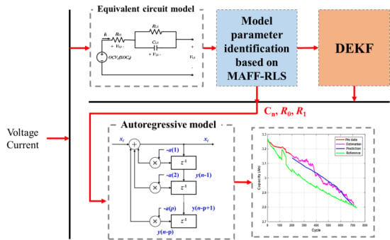
• Adaptive model: In the adaptive battery model, the ohmic resistance, diffusion resistance, and OCV are estimated via MAFF-RLS. According to the estimated parameter, the adaptive ECM estimates the terminal voltage, $H_k$, and $C_k$ for calculating the Kalman gain. The estimated terminal voltage is applied to the proposed DEKF through an ECM error with the measured terminal voltage.
• SOC and capacity estimation: The DEKF estimates the SOC and capacity in parallel structure, as shown in Figure 10.

In this study, the DEKF was not only used for estimating the state of the battery (SOC and capacity) but also applied to the prediction model in real-time (except for the initial value). The proposed algorithm identifies the parameters according to the MAFF-RLS. These parameters are applied to the DEKF and prediction models.

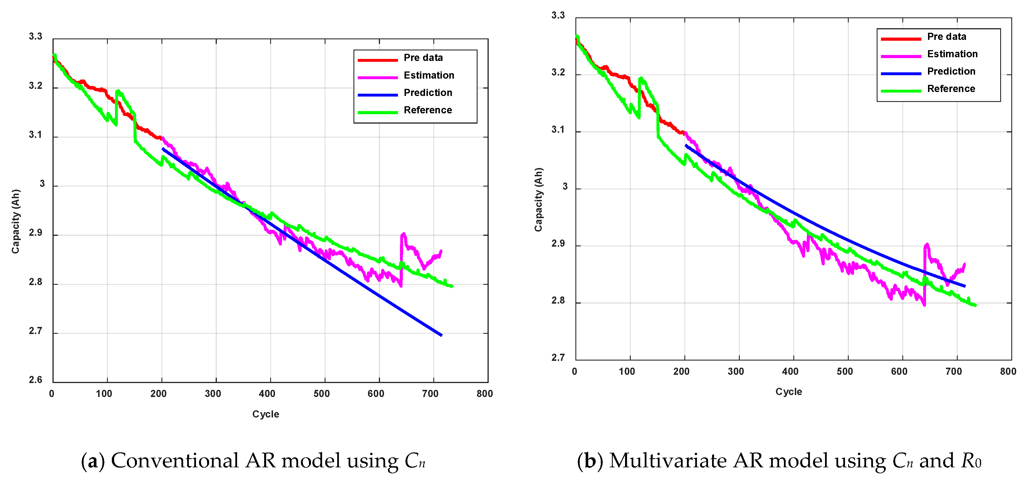
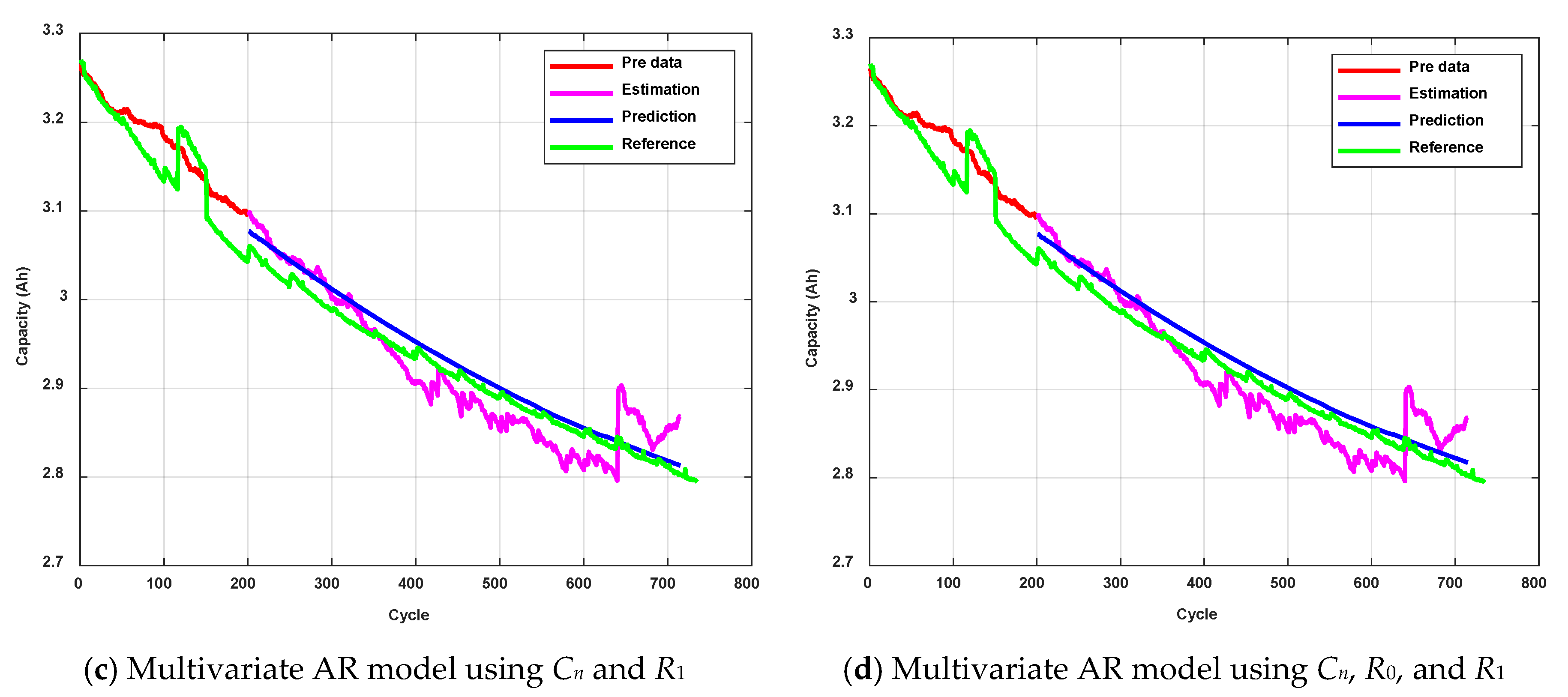
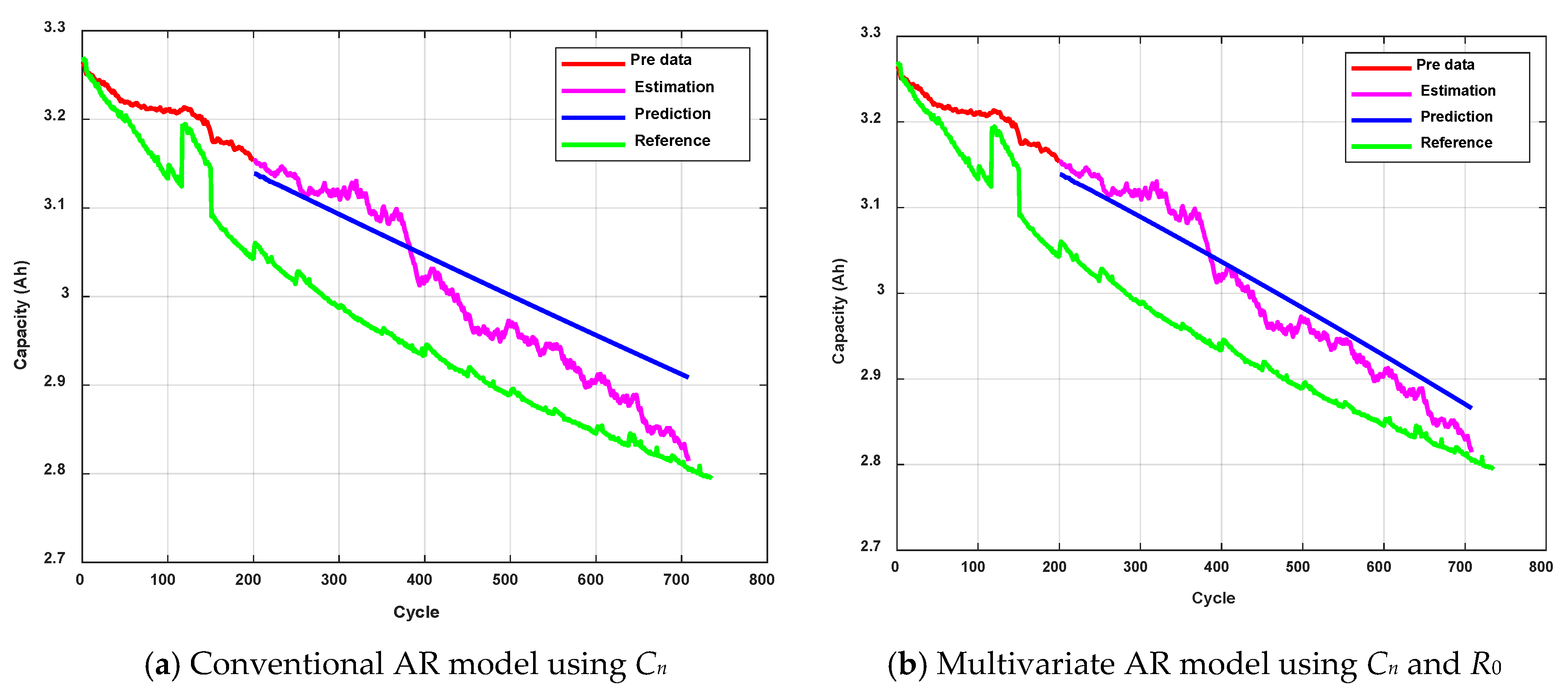
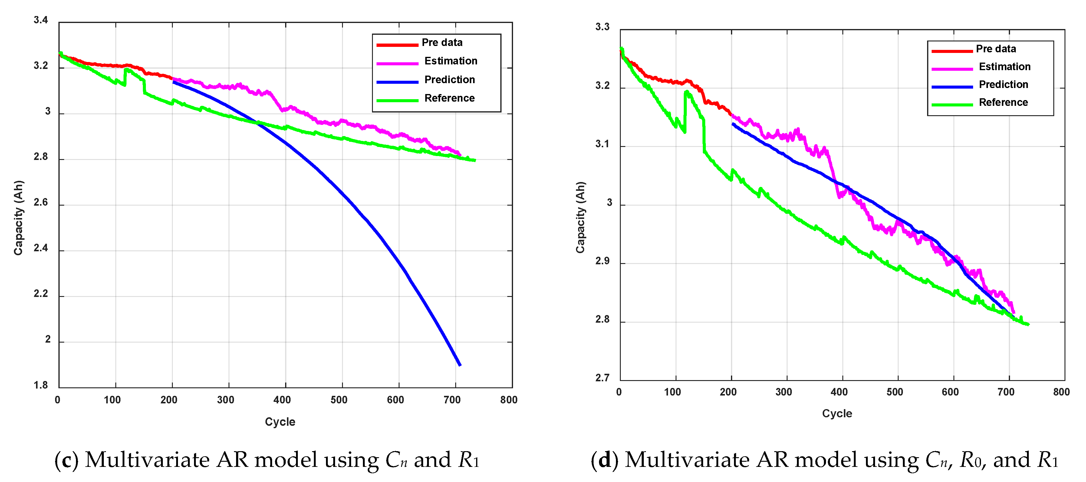
3.4. Autoregressive (AR) Model

The time-series approach helps predict the capacity loss without the complete aging data because the prediction model for time-series data assumes that the predicted data are related to past data. The AR model represents the current variable using the linear relationship of the previous time variable, as follows.

$$x(t)=a_1{x}_{t-1}+a_2{x}_{t-2}+\cdots +a_p{x}_{t-p}+{\epsilon }_t$$

(33)

where p represents the model order, which indicates the number of past data. a_p is a coefficient and ε represents white noise with zero mean.

The conventional AR model cannot predict nonlinear trends. Long et al. [36] used an AR model based on particle swarm optimization to determine the optimal order. Because the AR model is affected by the previous trend, the prediction result for the capacity fading is characterized by a linear trend. To overcome the limitation of the AR model, Liu et al. [37] proposed an AR model that considers two capacity degradation trends fitting different aging curves. However, in conventional studies, the capacity value was not feasible because it was measured via an under restricted experimental condition [12,26]. These findings indicate the following. First, the statistical model requires a large amount of experimental data to fit the capacity fading and additional nonlinear factor. Second, the measurement value in the experiment is not useful in real applications because the capacity changes, according to the SOC, depth of discharge (DOD), cycle, C-rate, etc. Lastly, if the variability of the battery capacity is nonlinear, it is difficult to predict using a linear relationship.

3.5. Integrated Model

For the previously mentioned AR model, the estimation and capacity prediction results were dependent on the accuracy of the measured data and the selection of the HI. In this study, the capacity was predicted using the multivariate AR model and the HI. The capacity for the next 500 cycles was predicted according to the capacity in the previous 200 cycles. The multivariate AR model combining R₀ and R_diff prediction data, which was expected to have strong correlation with capacity, was used for the AR model. The equation for predicting the capacity was as follows.

$$C_{n,t}={\displaystyle \sum _{\tau =1}^p{a}_t{C}_{n,t-\tau }}+b\cdot R_{0,t}+c\cdot R_{1,t}+{\epsilon }_t$$

(34)

where t represents the prediction time, C_n,t−τ is the index value of the previous 200 cycles data from the prediction time, and p represents the number of previous load values used. The prediction for 500 cycles was performed by increasing the prediction time through the iterative multivariate regression model and the previous predicted value was used when there was no previous measured load value.

4. Results and Discussion

The capacity prediction result was compared with the measured capacity and the estimated capacity from the SOC and SOH joint estimator (DEKF). These simulations were implemented for two cases: the measured capacity and estimated capacity of the DEKF. To validate the multivariate AR model and integrated model, the capacity prediction results were compared according to the variable numbers used for defining the AR model. Then, the performance for the two cases was evaluated using the mean absolute percentage error (MAPE), which was defined as follows.

$$MAPE=\frac{1}{N}{\displaystyle \sum _{k=1}^N\frac{\left|R_k-F_k\right|}{\left|R_k\right|}}\times 100$$

(35)

where R_k is the reference value and F_k is the forecast value.

As shown in Figure 11, the simulation results depended on which variable was applied to the AR model. The red line represents the measured capacity for fitting the data using 200 cycles that were obtained from the experimental data. The blue line represents the prediction results and the green line represents the reference. Figure 11a shows the prediction results obtained using only capacity data for the AR model. The prediction results exhibited a linear trend because the approximate capacity trend was almost linear in the 200 cycles. The MAPE for these results was 4.4006%. Figure 11b shows the results obtained using the capacity and ohmic resistance (R₀). Although the MAPE was 1.0606%, the prediction error increased exponentially with the cycle number. According to Figure 11c,d, the prediction results were more reliable, as the MAPE was 0.5324% and 0.4165%, respectively. This indicates that, in addition to the capacity and R₁, R_diff reflects the nonlinear characteristics of capacity prediction.

The prediction results of the AR model utilizing the estimated capacity from the DEKF are shown in Figure 12. The red and purple lines represent the estimated capacity. The average MAPE was under 1%. The prediction result in Figure 12a is similar to that in Figure 12a obtained using the estimated capacity only. The MAPE of the prediction results was 1.4518%, and the performance of prediction model was higher than that achieved using the measured capacity because the overall trend between 50 and 200 cycles tended to decrease, but the estimated capacity increased and decreased repeatedly. When R₀ and R₁ were applied to the AR model, the prediction results were superior to those obtained using the capacity only, as shown in

Table 3. Comparison of the mean absolute percentage error (MAPE).

	Cn	Cn + R0	Cn + R1	Cn + R0 + R1
Experiment (%)	4.4006	1.0606	0.5324	0.4165
Case 1 (%)	1.4518	0.7302	0.4566	0.5183
Case 2 (%)	3.6067	3.0266	9.3908	2.5599

.

The underestimated capacity of DEKF is selected in order to determine the HI, as shown in Figure 13. The underestimated capacity has a more nonlinear trend because this value fluctuates and the accuracy decreases more than Figure 12. In Figure 13a,b, the prediction results are almost linear and MAPE is 3.6067% and 3.0266%, respectively. Thus, it seems that the other parameter is required for predicting the nonlinear characteristics and enhancing the prediction performance. When the diffusion resistance is applied to the multivariate AR model, the prediction result has weakening performance than other results, as shown in Figure 13c, which represents the result of the multivariate AR model and the MAPE is 9.3908%. If two resistances (R₀ and R₁) are applied to the AR model at the same time, the MAPE is improved to 2.55%. In particular, it can be seen that the prediction performance is improved by changing the slope from about 500 cycles, as shown in Figure 13d.

As indicated by the foregoing simulation results, the capacity prediction results depend on the accuracy of the capacity data and the multivariate HI, which indicates the nonlinear trend of the prediction results. Thus, the prediction performance is highly dependent on selecting the appropriate experimental data and HI. The limitation of the AR model that the prediction result is linear can be resolved by applying another HI. However, the measured capacity cannot be used in real applications because the capacity is only measured under restricted experimental conditions. Therefore, in this study, the AR model was integrated with the joint estimator to estimate the SOC and SOH.

5. Conclusions

In practical applications, it is difficult to determine the appropriate HI and capacity because of the fluctuation of the battery parameters with the aging of the battery. The battery cycle is difficult to determine according to the operating range of applications. Hence, in this study, capacity data were obtained from a real-time estimator for predicting the capacity loss. The multivariate AR model and DKEF were integrated for real-time applications. The HI was estimated via MAFF-RLS, which was synchronized with the DEKF. Two resistances of the battery were applied to the AR model to reflect the nonlinear characteristics of capacity reduction. These resistances were estimated by the ARX model and MAFF-RLS to be utilized for the HI. Additionally, to overcome the limitations of existing methods predicted using measurement data, integration of the multivariate AR model and DEKF was necessary to estimate the capacity values in real-time.

According to the simulation results, the capacity prediction performance depends on aging factors related to the battery capacity. If the accuracy of the capacity value is increased, better performance can be achieved. Therefore, the capacity is the factor with the greatest effect on the prediction performance. However, for practical applications, the AR model should utilize the capacity estimated by a real-time estimator. Future research plans are as follows. First, a significant HI, such as the discharging rate or temperature, will be applied to the AR model since the lifespan is affected by these factors. Second, data-driven methods will be utilized for optimizing both the prediction model and HI. Our technique can be applied to a wide range of data-driven methods by adopting the adaptive controller that can estimate the optimal battery parameters in real-time. Third, since the proposed method utilized the adaptive controller and parameter identification, it has the potential to contstruct the new model for the next generation battery, which has different characteristics.

References

1. IRENA. Electricity Storage and Renewables: Costs and Markets to 2030; International Renewable Energy Agency: Abu Dhabi, United Arab Emirates, 2017. [Google Scholar]
2. International Renewable Energy Agency (IRENA). Global Energy Transformation: A Roadmap to 2050, 2019 ed.; IRENA: Abu Dhabi, United Arab Emirates, 2019. [Google Scholar]
3. Mauger, A.; Julien, C.M.; Paolella, A.; Armand, M.; Zaghib, K. Building better batteries in the solid state: A review. Materials 2019, 12, 3892. [Google Scholar] [CrossRef] [PubMed] [Green Version]
4. Bloomberg New Energy Finance. Energy Storage Outlook 2019; Bloomberg New Energy Finance Publication: Paris, France, 2019. [Google Scholar]
5. Dunn, B.; Kamath, H.; Tarascon, J.M. Electrical energy storage for the grid: A battery of choices. Science 2011, 334, 928–935. [Google Scholar] [CrossRef] [PubMed] [Green Version]
6. World Energy Council. Energy Storage Monitor Latest Trends in Energy Storage; World Energy Council: London, UK, 2019; p. 15. [Google Scholar]
7. Bloomberg New Energy Finance. Available online: https://about.bnef.com/blog/behind-scenes-take-lithium-ion-battery-prices/ (accessed on 5 May 2019).
8. Ren, H.; Zhao, Y.; Chen, S.; Wang, T. Design and implementation of a battery management system with active charge balance based on the SOC and SOH online estimation. Energy 2019, 166, 908–917. [Google Scholar] [CrossRef]
9. Garche, J.; Karden, E.; Moseley, P.T.; Rand, D.A. (Eds.) Lead-Acid Batteries for Future Automobiles; Elsevier: Amsterdam, The Netherlands, 2017; pp. 133–146. [Google Scholar]
10. Kwiecien, M.; Schröer, P.; Kuipers, M.; Sauer, D.U. Current research topics for lead–acid batteries. In Lead-Acid Batteries for Future Automobiles; Elsevier: Amsterdam, The Netherlands, 2017; pp. 133–146. [Google Scholar]
11. Wu, J.; Wang, Y.; Zhang, X.; Chen, Z. A novel state of health estimation method of Li-ion battery using group method of data handling. J. Power Sources 2016, 327, 457–464. [Google Scholar] [CrossRef]
12. Wu, J.; Zhang, C.; Chen, Z. An online method for lithium-ion battery remaining useful life estimation using importance sampling and neural networks. Appl. Energy 2016, 173, 134–140. [Google Scholar] [CrossRef]
13. Kang, B.O.; Lee, M.; Kim, Y.; Jung, J. Economic analysis of a customer-installed energy storage system for both self-saving operation and demand response program participation in South Korea. Renew. Sustain. Energy Rev. 2018, 94, 69–83. [Google Scholar] [CrossRef]
14. Gruber, P.W.; Medina, P.A.; Keoleian, G.A.; Kesler, S.E.; Everson, M.P.; Wallington, T.J. Global lithium availability: A constraint for electric vehicles? J. Ind. Ecol. 2011, 15, 760–775. [Google Scholar] [CrossRef]
15. Lucu, M.; Martinez-Laserna, E.; Gandiaga, I.; Camblong, H. A critical review on self-adaptive Li-ion battery ageing models. J. Power Sources 2018, 401, 85–101. [Google Scholar] [CrossRef]
16. Maheshwari, A.; Paterakis, N.G.; Santarelli, M.; Gibescu, M. Optimizing the operation of energy storage using a non-linear lithium-ion battery degradation model. Appl. Energy 2020, 261, 114360. [Google Scholar] [CrossRef]
17. Sun, Y.; Hao, X.; Pecht, M.; Zhou, Y. Remaining useful life prediction for lithium-ion batteries based on an integrated health indicator. Microelectron. Reliab. 2018, 88, 1189–1194. [Google Scholar] [CrossRef]
18. Xiong, R.; Zhang, Y.; Wang, J.; He, H.; Peng, S.; Pecht, M. Lithium-ion battery health prognosis based on a real battery management system used in electric vehicles. IEEE Trans. Veh. Technol. 2018, 68, 4110–4121. [Google Scholar] [CrossRef]
19. Zheng, Y.; Qin, C.; Lai, X.; Han, X.; Xie, Y. A novel capacity estimation method for lithium-ion batteries using fusion estimation of charging curve sections and discrete Arrhenius aging model. Appl. Energy 2019, 251, 113327. [Google Scholar] [CrossRef]
20. Liu, D.; Zhou, J.; Liao, H.; Peng, Y.; Peng, X. A health indicator extraction and optimization framework for lithium-ion battery degradation modeling and prognostics. IEEE Trans. Syst. Man Cyber. Syst. 2015, 45, 915–928. [Google Scholar]
21. Zhou, Y.; Huang, M.; Chen, Y.; Tao, Y. A novel health indicator for on-line lithium-ion batteries remaining useful life prediction. J. Power Sources 2016, 321, 1–10. [Google Scholar] [CrossRef]
22. Verma, P.; Maire, P.; Novák, P. A review of the features and analyses of the solid electrolyte interphase in Li-ion batteries. Electrochim. Acta 2010, 55, 6332–6341. [Google Scholar] [CrossRef]
23. Jung, B.; Lee, B.; Jeong, Y.C.; Lee, J.; Yang, S.R.; Kim, H.; Park, M. Thermally stable non-aqueous ceramic-coated separators with enhanced nail penetration performance. J. Power Sources 2019, 427, 271–282. [Google Scholar] [CrossRef]
24. Sarkar, A.; Shrotriya, P.; Chandra, A.; Hu, C. Chemo-economic analysis of battery aging and capacity fade in lithium-ion battery. J. Energy Storage 2019, 25, 100911. [Google Scholar] [CrossRef]
25. Krewer, U.; Röder, F.; Harinath, E.; Braatz, R.D.; Bedürftig, B.; Findeisen, R. dynamic models of Li-Ion batteries for diagnosis and operation: A review and perspective. J. Electrochem. Soc. 2018, 165, A3656–A3673. [Google Scholar] [CrossRef]
26. Pastor-Fernández, C.; Uddin, K.; Chouchelamane, G.H.; Widanage, W.D.; Marco, J. A comparison between electrochemical impedance spectroscopy and incremental capacity-differential voltage as Li-ion diagnostic techniques to identify and quantify the effects of degradation modes within battery management systems. J. Power Sources 2017, 360, 301–318. [Google Scholar] [CrossRef]
27. Gomez, J.; Nelson, R.; Kalu, E.E.; Weatherspoon, M.H.; Zheng, J.P. Equivalent circuit model parameters of a high-power Li-ion battery: Thermal and state of charge effects. J. Power Sources 2011, 196, 4826–4831. [Google Scholar] [CrossRef]
28. Pan, H.; Lü, Z.; Wang, H.; Wei, H.; Chen, L. Novel battery state-of-health online estimation method using multiple health indicators and an extreme learning machine. Energy 2018, 160, 466–477. [Google Scholar] [CrossRef]
29. Qiu, X.; Wu, W.; Wang, S. Remaining useful life prediction of lithium-ion battery based on improved cuckoo search particle filter and a novel state of charge estimation method. J. Power Sources 2020, 450, 227700. [Google Scholar] [CrossRef]
30. Xue, Z.; Zhang, Y.; Cheng, C.; Ma, G. Remaining useful life prediction of lithium-ion batteries with adaptive unscented kalman filter and optimized support vector regression. Neurocomputing 2020, 376, 95–102. [Google Scholar] [CrossRef]
31. Yang, F.; Wang, D.; Zhao, Y.; Tsui, K.L.; Bae, S.J. A study of the relationship between coulombic efficiency and capacity degradation of commercial lithium-ion batteries. Energy 2018, 145, 486–495. [Google Scholar] [CrossRef]
32. Duong, V.H.; Bastawrous, H.A.; Lim, K.; See, K.W.; Zhang, P.; Dou, S.X. Online state of charge and model parameters estimation of the LiFePO4 battery in electric vehicles using multiple adaptive forgetting factors recursive least-squares. J. Power Sources 2015, 296, 215–224. [Google Scholar] [CrossRef]
33. Zilberman, I.; Ludwig, S.; Jossen, A. Cell-to-cell variation of calendar aging and reversible self-discharge in 18650 nickel-rich, silicon–graphite lithium-ion cells. J. Energy Storage 2019, 26, 100900. [Google Scholar] [CrossRef]
34. Wassiliadis, N.; Adermann, J.; Frericks, A.; Pak, M.; Reiter, C.; Lohmann, B.; Lienkamp, M. Revisiting the dual extended Kalman filter for battery state-of-charge and state-of-health estimation: A use-case life cycle analysis. J. Energy Storage 2018, 19, 73–87. [Google Scholar] [CrossRef]
35. Plett, G.L. Extended Kalman filtering for battery management systems of LiPB-based HEV battery packs: Part 3. State and parameter estimation. J. Power Sources 2004, 134, 277–292. [Google Scholar] [CrossRef]
36. Long, B.; Xian, W.; Jiang, L.; Liu, Z. An improved autoregressive model by particle swarm optimization for prognostics of lithium-ion batteries. Microelectron. Reliab. 2013, 53, 821–831. [Google Scholar] [CrossRef]
37. Liu, D.; Luo, Y.; Peng, Y.; Peng, X.; Pecht, M. Lithium-ion battery remaining useful life estimation based on nonlinear AR model combined with degradation feature. In Proceedings of the Annual Conference of the Prognostics and Health Management Society, Minneapolis, MN, USA, 23–27 September 2012; Volume 3, pp. 1803–1836. [Google Scholar]
Figure 1. Experimental platform of the battery.
Energies 13 02138 g001
Figure 2. Profiles obtained in the cycling test: (a) entire voltage profile and (b) voltage and current profile at one cycle.
Energies 13 02138 g002
Figure 3. Battery equivalent circuit model.
Energies 13 02138 g003
Figure 4. The battery state of charge (SOC) - open circuit voltage(OCV) test profile.
Energies 13 02138 g004
Figure 5. Method of parameter identification.
Energies 13 02138 g005
Figure 6. Comparison of the SOC-OCV curve between the fresh and aging condition.
Energies 13 02138 g006
Figure 7. Relationship between capacity and resistance.
Energies 13 02138 g007aEnergies 13 02138 g007b
Figure 8. Linear fitting and residual analysis of the capacity and ohmic resistance.
Energies 13 02138 g008
Figure 9. Linear fitting and residual analysis of the capacity and diffusion resistance.
Energies 13 02138 g009
Figure 10. Flowchart of the dual extended Kalman filter (DEKF).
Energies 13 02138 g010
Figure 11. Capacity prediction results obtained using the autoregressive (AR) model and the measured capacity.
Energies 13 02138 g011aEnergies 13 02138 g011b
Figure 12. Capacity prediction results obtained using the AR model and dual extended Kalman filter (DEKF) (case 1).
Energies 13 02138 g012aEnergies 13 02138 g012b
Figure 13. Capacity prediction results obtained using the AR model and DEKF (case 2).
Energies 13 02138 g013aEnergies 13 02138 g013b