Experimental Design, Instrumentation, and Testing of a Laboratory-Scale Test Rig for Torsional Vibrations—The Next Generation


Mewbourne School of Petroleum and Geological Engineering, The University of Oklahoma, Norman, OK 73019, USA
*
Author to whom correspondence should be addressed.
Energies 2020, 13(18), 4750; https://doi.org/10.3390/en13184750
Submission received: 11 August 2020
/
Revised: 3 September 2020
/
Accepted: 8 September 2020
/
Published: 11 September 2020
(This article belongs to the Special Issue Drilling Technologies for the Next Generations)
Abstract
:Drilling technology and specially drilling equipment has dramatically changed in the last 10 years through intensive and innovative technologies, both in terms of hardware and software. While engineers are focusing on safer, faster, and more reliable than ever technologies, big data and automation are currently considered the way forward to achieve these goals. Especially when automation concepts are proposed, the prior testing and qualification under a laboratory-controlled environment are mandatory. Drilling simulators have been hugely successful in training industry personnel and academic professionals. A big reason for its success lies in the seamless integration of hardware and software to include an interactive user interface. Physical experimental simulators have the advantage of exposing the user with visual and auditive aids to better understand the real process. This paper provides an insight into the construction and results obtained using a dedicated laboratory setup, which is also configured to various levels of automation. The setup is capable of safely recreating drilling vibrations that occur in wells, including stick-slip vibrations, which are detrimental in nature. With advanced sensor capabilities, the impact of proper sampling rates on the diagnosis of stick-slip vibrations has been analyzed in the paper. The results show that these vibrations are not only dependent on drilling parameters, such as rotational speed (RPM), torque, and weight on bit, but also on stick-slip parameters, such as bit sticking time period and frequency.
1. Introduction
Field experiments have played a crucial role in investigating every aspect of drilling. Some examples include an examination of drill string vibrations [1], the efficiency of downhole data transmission [2], and evaluation of bit performance [3]. While the presence of these field-testing facilities across the world has played a big role in the advancement of drilling technologies, these facilities have high operational costs along with the lack of a controlled testing environment [4]. Downscaled laboratory experiments, on the other hand, provide an efficient testing mechanism because of the repeatability of testing conditions in a controlled, low-risk environment. Moreover, the ease of construction and operation of laboratory scaled experiments has enabled operators and academic institutions to produce conclusive research on drilling processes. Drilling automation remains one such promising avenue.
As the drilling industry moves towards automation to increase productivity and efficiency, downscaled experimental test rigs provide an ideal setting for the safe implementation of automation techniques. As seen in Table 1, each level of automation has a designated degree of human and computer control, with level 1 being fully human-controlled, and level 10 being fully computer-controlled or autonomous. Drillbotics, an annual international competition, has continuously challenged university students globally to design, build, and test an autonomous lab scaled drilling rig that successfully drills complex rock samples. Students and faculty have worked together to implement an impressive automation capability up till level 9 [5]. This advancement in automation not only calls for innovative rig designs to tackle real-world issues within the realms of downscaling but also a robust understanding of sensor integration, data measurement, and control algorithms. However, this information is not readily available in the literature.
A review of experimental test rigs built to analyze drill string vibrations includes an extensive list of laboratory-scale test rigs built in the last two decades was presented by Srivastava and Teodoriu [7]. While the review contains an extensive analysis of the design features of the existing rigs, the authors do not mention the instrumentation aspect of the test rigs. This is due to the unavailability of this information, along with no standardized approach to instrumentation. This ambiguity in the appropriate sensor integration, adequate data sampling, control algorithms, and human-machine interfacing needs to be addressed.
This paper attempts to fill the gap by providing a different dimension to the design of a laboratory scaled experimental test rig by elaborating on the process of instrumentation involved. In doing so, it provides a detailed integration of mechanical and electrical components of a test rig along with programming details and human-machine interfacing.
2. Experimental Approach
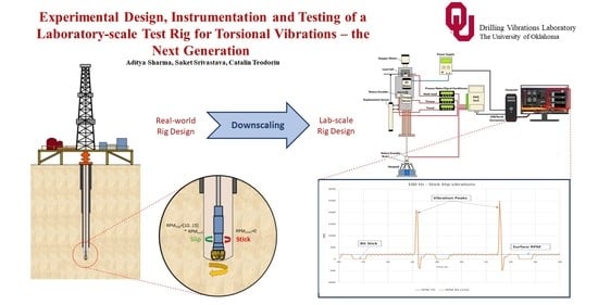
In what follows, the experimental approach used in this work is shown. First, an experimental test rig has been described, followed by the measurement and data collection. The experimental test rig described in this paper is present at the drilling vibration laboratory at the University of Oklahoma. It is one of the most advanced experimental setups for measuring torsional vibrations, including stick-slip analysis (Srivastava and Teodoriu, 2019). In the experimental setup, the real scale drill pipe length of 450 m is scaled down to 15 m using a scaling factor of 1:30. Table 2 lists the scaled values of different design parameters. To incorporate reduced torsional stiffness due to downscaling, a PVC drill pipe of diameter 0.125 inches is used.
While this paper gives a brief review of the mechanical construction of the test rig, it elaborates extensively on the integration of electrical components into the system. The paper further explains the intricacies of data acquisition and the utilization of LabVIEW in programming the control architecture of the setup. All signals are collected by a Digital Analog card (DAQ) and stored on the process computer.
2.1. Mechanical Components
The mechanical components of the rig can be subdivided into three major components, namely, top drive, drill string, and bottom hole assembly.
2.1.1. Top Drive
The top drive of the experimental setup consists of an 18V DC motor for providing rotational energy to the drill string and a stepper motor with a lead screw mechanism for hoisting and weight on bit (WOB) control. This can be seen in Figure 1. The DC motor helps provide a constant voltage under a current limit for smooth torque output. The sensors installed in the top drive have been discussed at length in the electrical component of the rig layout.
2.1.2. Drill String
The drill string used for the experiments shown in this paper consists of a thin PVC pipe of 4 mm Outer Diameter (OD) and stands at an impressive 49 ft in length, thus helping to achieve a downscaling ratio of 1:30. Figure 2 shows the length span of the drill string in the laboratory. Furthermore, PVC is chosen as the material in place of aluminum or steel for drill pipe material. Due to PVC’s lower torsional stiffness, torsional vibrations are more readily generated for a given value of downhole torque in the setup.
2.1.3. Bottom Hole Assembly
The torque generated at the bit is required to induce torsional vibrations in the drill string. It can be generated by actual drilling of a rock sample or by a braking system that provides torque at bit. Considering how repeatability of results is a vital component of testing, the braking system is preferred. The experimental setup includes a state-of-the-art hexapod braking system that is capable of 6 axis motion while braking. This system uses an electromagnetic brake to induce torque in the bottom hole assembly. The system further connects to a rotary encoder that measures precise angular movement during testing.
2.2. Electrical Components
The rig is equipped with several sensors and actuators that are described below.
2.2.1. Sensors
- Load cell: The load cell used to measure the hook load is a strain gauge-based bridge transducer and is used to measure the weight on bit by subtracting the weight of the string (see Figure 3). The low magnitude voltage output signal from the load cell is amplified by a signal processor and then is fed to the DAQ device. Specifications include:
- Range: 0–25 Lb.
- Excitation: 10–15 Vdc.
- Output: 2 mV/V nominal.
- Accuracy: ±1.0% FSO linearity, hysteresis, repeatability combined.
- Torque sensor: Like the load cell, the torque sensor is also a strain gauge-based bridge transducer with a low magnitude voltage output signal. The sensor is shown in Figure 4. The output from this sensor must also be amplified by a signal processor before being fed to the DAQ device. It is placed just below the top drive and measures the torque on the drill string. Specifications include:
- Range: 0–1.41 N.m.
- Excitation: 20 Vdc maximum.
- Output at full scale: 2.0 mV/V nominal.
- Linearity: 0.10% FS (Full Scale).
- Hysteresis: 0.10% FS.
- Rotary encoder: Two quadrature rotary encoders are used to measure the top and bottom RPM and the direction (anti-clockwise or clockwise). Both the top and bottom encoders are 500 PPR, i.e., they generate 500 digital pulses per revolution. Figure 5 shows one of the two encoders used. Specifications include:
- Excitation: 5–24 Vdc.
- PPR: 500.
- Max shaft speed: 8000 RPM.
- Displacement sensor: This is a potentiometer-based stroke pull rod linear position displacement sensor and is used to measure the vertical distance traveled (Figure 6). It can measure up to 300 mm displacement. Specifications include:
- Excitation: 5–24 Vdc.
- Resistance: 5K Ohm.
- Linearity: +/− 0.05%.
- Range: 0–300 mm.
2.2.2. Actuators
- DC motor: A DC is used as the top drive motor for providing rotational energy to the drill string. Specifications include:
- Input voltage: 0 to 18 V
- Stepper motor: A programmable stepper motor is used for the hoisting mechanism (see Figure 7). Specifications include:
- Input voltage: 24–48 Vdc
- Holding torque: 0.88 N.m
- Steps/Rev: Programmable, set to 25,000
- NEMA size: 23
2.3. Data Acquisition and Software
This section talks about the hardware and software used to acquire and process the data collected from the setup.
2.3.1. Data Acquisition Device
A 16-bit multi-function data acquisition device (DAQ), with a sampling rate of up to 250 kHz, is used. Raw data from the analog sensors in the form of dc voltage ranging between 0 and 10 V is read at the analog inputs, and digital data from the rotary encoders is read at the digital inputs of the DAQ. The data collected by the device is processed in LabVIEW.
2.3.2. Arduino Mega
Arduino Mega is a single board ATmega2560-based microcontroller and has multiple analog and digital I/Os. The Mega has been originally used in the setup, specifically to read the digital signals from the rotary encoders and to convert those signals to usable RPM and direction string data. This string data is transmitted to NI LabVIEW using serial communication between the Arduino Mega and the computer running NI LabVIEW. The Arduino Mega is capable of handling up to four rotary encoders but has a slower processing speed because of which the sampling frequency is experimentally tested to be limited to 10 Hz. With higher sampling frequencies, the data output is unreliable.
2.3.3. Process Meter/Signal Conditioner
The two strain-gauge based sensors—load cell and torque sensor—have a signal output in millivolts (mV). Thus, a signal conditioner must be used for each of these sensors. The signal conditioner scales the output to the 0–10 V range, which can be read by the data acquisition device.
Three process meters with built-in signal conditioners and programmable displays are used in the setup. The raw output from the load cell, torque sensor, and the displacement sensor is passed through the process meters before it goes to the data acquisition device. This allows for real-time measurement of WOB, torque, and displacement on the process meter display. Furthermore, in the case of the load cell and the torque sensor, it scales the output before it reaches the DAQ.
2.3.4. LabVIEW
LabVIEW is a system-design platform, which uses a graphical programming language to design systems. It is widely used for data acquisition, instrumentation, and control and automation. It is very easy to integrate with a variety of data acquisition platforms. It supports various communication protocols to send and receive data.
LabView has been used to program and control the setup and to develop the human-machine interface (HMI). It collects data from the DAQ, processes it, and then displays the process parameters on the HMI and provides the ability to control the two actuators in the system: the top drive motor and the stepper motor used for hoisting.
2.4. Sensor Calibration
The load cell, torque sensor, and the displacement sensor have a linear response to the input and are calibrated experimentally using known inputs and recording the respective voltage output responses to the inputs. Linear plots for the three sensors are generated, and the equations of the trendline are used to derive the three physical quantities: hook load, torque, and displacement. The equations are listed below:
Load cell equation:
Y = 134.21x − 120.24
Torque sensor equation:
y = 1.5935x − 1.4591
Displacement sensor equation:
y = 125.85x − 250.57
2.5. Calculating RPM Using Rotary Encoder Data
A rotary encoder is an electro-mechanical device, which converts the angular rotation of a shaft to an electrical signal. The rotary encoders used in the setup have a digital output and one complete rotation of the shaft generates 500 digital pulses. These digital pulses can be used to calculate the RPM with which the shaft rotates [8]. The method to derive RPM from the digital signal is described below.
where Δp is the change in the pulse count of the encoder from time ‘t1’ to time ‘t2’ (time in ms).
t = t2 – t1
PPR is the total number of pulses the encoder generates on completing one revolution of the shaft. Therefore,
The left side of the equation is the RPM of the encoder shaft. Therefore,
where,
is the total number of pulses generated in time ‘t’ (in ms)
is the pulses per revolution of the encoder,
is the sampling frequency in Hz.
3. Programming the Setup
As stated before, LabView has been used to program and control the setup. The LabVIEW code consists of four parallel running loops, each of which controls a specific part of the setup. The four loops are described below.
3.1. Sensor Input and Calibration Loop
This loop reads the analog inputs on the USB-6210 and outputs the torque, weight on bit, and the position displacement on the HMI. This is done using the linear equations generated from the calibration of the sensor. The equations are programmed in the loop and the analog voltage values are used as input to output the corresponding physical quantities. For example, for the torque sensor, Equation (2) is implemented in the LabVIEW code, as shown in Figure 11. The loop runs at a sampling frequency set by the user and is also capable of saving the data points in the file. Figure 12 shows a screenshot of this loop.
3.2. Motor Control Loop
This loop controls the variable power supply, which powers the DC top drive motor. The DC motor can run on a maximum input voltage of 18 V, changing the input voltage to the RPM of the motor. Thus, a variable power supply is used to control the RPM of the top drive motor. LabVIEW communicates with the variable power supply using serial commands through a USB serial communication link. The loop controls the voltage output of the variable power supply and reads the current drawn from the supply, which is used to calculate the power drawn by the dc motor. Figure 13 is a screenshot of the motor control loop.
3.3. Hoisting System Loop
This loop controls the NI ISM-7411 stepper motor, which is used for the hoisting system. The motor communicates with LabVIEW via an Ethernet connection and uses the NI SoftMotion module.
3.4. Rotary Encoder Loop
Initially, the digital output from the encoders is connected to the digital inputs on the Arduino Mega. The processed data from the top and bottom direction RPM and angular position are derived and transmitted to the LabVIEW code via a serial port. Due to the lower processing power of the Arduino Mega, the sampling frequency for the derived quantities is limited to 10 Hz. To achieve higher sampling frequencies, the digital output of the encoder is directly connected to the digital inputs on the USB-6210. The one limitation of doing this is that no more than two rotary encoders can be used in the setup since the USB-6210 only has four digital inputs.
With the encoders connected to the USB-6210, the digital signals are read in LabVIEW, and Equation (4) is programmed in the rotary encoder loop shown in Figure 14.
4. The HMI Design
Drilling simulators have been hugely successful in training industry personnel and academic professionals. A big reason for its success lies in the seamless integration of hardware and software to include an interactive user interface. While the simulator replicates a physical process in the real world, the user interface can be adjusted to the required complexity. The user interface can vary from those used in commercial simulators for industry training [9] to academic simulators for the pipe running process [10]. The HMI shown in Figure 15 has been inspired by such sources to have adequate complexity for the objective of evaluating torsional vibrations.
The HMI has a user-friendly design and layout. It displays all the process parameters in real-time and has the controls for the top drive and the hoisting system. The next sub-sections give a better understanding of the individual components in the design.
4.1. Real-Time Process Parament Gauges and Indicators
Figure 16 shows the different gauges and indicators on the HMI. The position, top RPM, bottom RPM, torque, hook load, and weight can be easily read from the gauges or the indicators in real-time.
4.2. Controls and Plots
The HMI enables the user to control the RPM and the weight on bit. To control the RPM of the top drive, the user can change the value of the input voltage to the motor using a slider or a numeric input. The real-time power drawn by the motor is also displayed on the HMI. The RPM control panel is shown in Figure 17.
The weight on bit can be adjusted through the hoisting mechanism control panel shown in Figure 18. By moving up, the weight on bit is increased, and by moving down, the weight can be decreased. The change in weight on bit is related to the tension in the string. The user can set the toggle switch to move up or move down position and press the start/stop button to move up or down.
The simulation data can be saved by switching on the ‘Save Data’ switch. This saves the process parameters generated during the simulation in a file. The sampling frequency can also be set to the desired value. There is also a red stop button, which stops the actuators and the simulation on one click. These controls can be seen in Figure 19.
On the right side of the HMI, three plots (Figure 20) are present. These plots plot the top and bottom RPM, torque, and weight on bit in real-time and are used to keep track of these parameters as they change with time.
5. Experiments and Results
A good way to evaluate the integration of electrical and mechanical components discussed above is to perform experiments with the setup. The test rig is designed to measure a range of torsional vibrations, including stick-slip vibrations. As seen in Figure 1, the setup consists of a torque sensor and rotary encoder at the surface and a rotary encoder and electromagnetic brake at the bit. The electromagnetic brake is responsible for generating torque at the bit. When the torque at bit nears the torque generated at the surface, the bit undergoes a sticking mechanism, where the RPM drops to zero. The removal of this torque at bit results in a sudden release of energy at the bit with a powerful increment in rotational energy. Since this mechanism is dependent on the sticking period, which can vary from 0.5 s to 5 s, the sensors are sampled between 1 and 100 Hz to record the changes in bit RPM.
Figure 21 provides an example of the range of experimental tests possible with the setup. The blue line depicts the surface RPM of 100, whereas the orange line marks the RPM at the bit. The positive and negative fluctuation of bit RPM around 100 depicts a clear case of torsional vibrations. Stick-slip situations can be observed when the bit RPM drops to zero. Stick-slip vibrations are analyzed for both low and high frequency depending on the period of stick and slip.
The experimental setup provides a unique combination of possible testing combinations that include:
- Controlling the input voltage for the DC motor to vary the RPM of the string.
- Utilizing the hoisting system to vary the tension in the string to set the required weight on bit. The experiments have been run between 500 g and 1000 g weight on bit.
- Introduction of controlled torque at the bit with an ability to vary bit sticking period.
- Ability to toggle data sampling rates between 1, 10, and 100 Hz.
The experimental tests have been performed to study the effect of rotational speed on stick-slip behavior and the impact of stick and slip period on torsional vibration pattern. Figure 22 compares the vibration signature for similar testing conditions with the only difference of surface RPM (100 and 200). The sticking period for each RPM case is further highlighted in the figure. On closer look, the stick period for 200 RPM is lower than the stick period for 100 RPM. This can be explained by the higher and quicker energy accumulation in the 200 RPM string to overcome the sticking bit torque. This confirms the industry practice to increase surface RPM during stick-slip vibrations. However, it can also be noted that the higher string RPMs also result in slightly higher peaks in vibration, as seen in Figure 22. Although the difference in vibration peaks for 200 RPM is not significantly different from 100 RPM peaks, it is worth keeping in mind. Interestingly, negative RPMs are also observed in the string, which is a result of the instantaneous release of energy buildup in the string.
Similarly, the sticking period due to torque at the bit is analyzed for a string rotating at 100 RPM. Figure 23 compares tests with exactly similar testing parameters except sticking period of 1 and 5 s. The torque at the bit for the different time durations remains the same. As discussed previously, the longer bit sticking period results in a higher energy accumulation in the string, which, in turn, causes higher energy release, as seen through taller peaks in vibration. Therefore, low-frequency stick-slip vibrations can result in serious damage to downhole tools and well trajectories, amongst other potential issues.
Most interestingly, the effect of sampling sizes in recognizing stick-slip vibrations is discussed in Figure 24. The figure is split into three plots of 1, 10, and 100 Hz. The surface RPM remains constant throughout the three plots with vast differences in bit RPM responses. The 1 Hz plot clearly misses the true signature of the stick-slip vibration with incomplete crests and troughs. When compared to the 10 Hz vibration data, the 1 Hz plot fails to capture the severity of the damaging peaks in vibration as well as the momentary sticking of the bit. The 10 Hz plot, on the other hand, highlights a momentary 1 s bit sticking phenomenon (22.8 s to 23.8 s) along with a negative peak in vibration. With an instantaneous bit RPM of 10 times the surface RPM, the 10 Hz plot gives insight into the actual peaks in vibrations observed. The data for 100 Hz is even more accurate and precise. While it performs better than both 1 and 10 Hz in capturing minute details like the string stabilization period after undergoing stick-slip vibrations, the stored data file also becomes substantially larger.
The experimentation of torsional vibrations proves that sampling rates are crucial for making informed decisions about the presence of severe vibrations during drilling. Although stick-slip vibrations are low-frequency vibrations, the tests also provide conclusive evidence to maintain a minimum sampling rate of 10 Hz to identify instantaneous peaks in downhole vibrations. Higher sampling rates are always preferable as long as data management and storage issues are taken care of.
6. Discussions
More than 300 tests have been performed on the new drilling simulator till the acceptance of this research paper. The simulator shows good performance in reproducing stick-slip vibrations and excellent repeatability of testing conditions. The experimental work presented in the paper is shortly discussed below.
The tests are performed at different rotational speeds undergoing the same experimental stick-slip conditions. This has helped in understanding the response of downhole RPM based on varying top drive rotational speeds. While comparing slip behavior in Figure 22, the downhole RPM shoots to more than 15 times the average surface RPM of 100 as compared to 15 times the average surface RPM of 200. This highlights how lower rotational speeds are more susceptible to torsional vibrations, specially detrimental vibrations observed in the form of stick-slip behavior. Lower rotational speeds also take longer to overcome the torque at the bit, as seen in Figure 22.
The tests are also performed for varying sticking periods and sensor sampling rates. The relation between bit sticking periods to peaks in vibrations is linear in nature. Higher bit sticking duration results in higher energy accumulation and higher peaks in bit RPM during the slip period. The experimental tests also provide insightful conclusions about the need to include higher sampling rates during measurement and diagnosis of torsional vibrations. As seen in Figure 24, the 1 Hz plot is successful in picking bit RPM vibration peaks of twice the surface RPM as compared to ten and fifteen times the surface RPM in 10 Hz and 100 Hz sampled data.
7. Conclusions
The novel experimental stick-slip simulator presented in this paper shows the necessity of good integration of hardware and software to achieve reliable results. The sensors and data acquisition rates play a critical role in the design of the experimental setup.
LabVIEW is used as the controlling software, given its flexibility and the research group’s vision to achieve higher levels of automation in the future.
Through experimental tests for stick-slip vibrations, the bottom assembly of the drill string is found to rotate up to 15 times the surface RPM. Furthermore, the signature string motion during stick-slip vibrations is also visualized.
Furthermore, a minimum sampling rate of 10 Hz is determined to better identify the severity of stick-slip vibrations in the system.
8. Future Improvements
The present setup is an open-loop control system and is at the second level of automation, which is the ‘Action support’ level. Future plans involve getting the system up to level 5 (Decision support), which is an intermediate level with both human and computer involvement. Intermediate levels of automation can perform better than the higher levels of automation, but the downside of removing human influence from the control system includes a possible loss of situational awareness [11]. To achieve level 5 automation, the open-loop control will have to be switched with closed-loop feedback control for the RPM and WOB control. This will be done with the use of proportional–integral–derivative (PID) controllers in LabVIEW.
Author Contributions
Conceptualization, C.T.; Methodology, C.T.; Formal Analysis, C.T., A.S., and S.S.; Experimental Work, C.T., A.S., and S.S.; Writing—Original Draft Preparation, A.S. and S.S.; Writing—Review and Editing, C.T., A.S., and S.S.; Supervision of Experiments, C.T. All authors have read and agreed to the published version of the manuscript.
Funding
This research was supported by the Helmerich and Payne LLC project at the University of Oklahoma.
Acknowledgments
We would like to thank Helmerich and Payne LLC for their amazing support. We also like to thank the University of Oklahoma and The Drilling Vibrations Laboratory for permission to publish the results.
Conflicts of Interest
The authors declare no conflict of interest.
Abbreviations
| RPM | Revolutions per minute |
| DC | Direct current |
| WOB | Weight on bit |
| OD | Outside diameter |
| PVC | Polyvinyl chloride |
| DAQ | Data acquisition |
| FSO | Full-scale output |
| FS | Full scale |
| PPR | Pulses per revolution |
| I/Os | Inputs/Outputs |
| HMI | Human-machine interface |
| PID | Proportional-integral-derivative (controller) |
Variables
| L | length (m) |
| D | diameter (inches) |
| ω | angular velocity (RPM) |
| ⍴ | density(g/cm3) |
| E | elasticity (Pa) |
| τ | motor torque (mNm) |
| KTOR | torsional stiffness (Nm/rad) |
| Δp | change in pulse count from the encoder in time ‘t’ |
| pt1 | pulse count at time ‘t1’ |
| pt2 | pulse count at time ‘t2’ |
| t | time (ms) |
| f | sampling frequency (Hz) |
References
- Finnie, I.; Bailey, J.J. An Experimental Study of Drill-String Vibration. ASME. J. Eng. Ind. 1960, 82, 129–135. [Google Scholar] [CrossRef]
- Reeves, M.E.; Payne, M.L.; Ismayilov, A.G.; Jellison, M.J. Intelligent Drill String Field Trials Demonstrate Technology Functionality; Society of Petroleum Engineers: Houston, TX, USA, 2005. [Google Scholar] [CrossRef]
- Dykstra, M.W.; Chen, D.C.-K.; Warren, T.M. Experimental Evaluations of Drill Bit and Drill String Dynamics; Society of Petroleum Engineers: Houston, TX, USA, 1994. [Google Scholar] [CrossRef]
- Raymond, D.W.; Elsayed, M.A.Y.P.; Kuszmaul, S.S. Laboratory simulation of drill bit dynamics using model based servohydraulic controller. J. Energy Resour. Technol. 2008, 130. [Google Scholar] [CrossRef]
- Zarate-Losoya, E.; Cunningham, T.; El-Sayed, I.; Noynaert, S.F.; Florence, F. Lab-Scale Drilling Rig Autonomously Mitigates Downhole Dysfunctions and Geohazards through Bit Design, Control System and Machine Learning; Society of Petroleum Engineers: Houston, TX, USA, 2018. [Google Scholar] [CrossRef]
- Endsley, M.R.; Kaber, D.B. Level of automation effects on performance, situation awareness and workload in a dynamic control task. Ergonomics 1999, 42, 462–492. [Google Scholar] [CrossRef] [PubMed] [Green Version]
- Srivastava, S.; Teodoriu, C. An extensive review of laboratory scaled experimental setups for studying drill string vibrations and the way forward. J. Pet. Sci. Eng. 2019, 182, 106272. [Google Scholar] [CrossRef]
- Briz, F.; Cancelas, J.A.; Diez, A. Speed measurement using rotary encoders for high performance AC drives. In Proceedings of the IECON’94—20th Annual Conference of IEEE Industrial Electronics, Bologna, Italy, 5–9 September 1994; Volume 1, pp. 538–542. [Google Scholar] [CrossRef]
- Drilling Systems Website. Available online: http://www.drillingsystems.com (accessed on 5 August 2020).
- Srivastava, S.; Ichim, A.; Teodoriu, C. Development of Next Level Drilling Simulator Using Multiple User Interaction Concepts. In Proceedings of the Offshore Technology Conference, Houston, TX, USA, 3 May 2018. [Google Scholar] [CrossRef]
- Endsley, M.R.; Kiris, E.O. The Out-of-the-Loop Performance Problem and Level of Control in Automation. Hum. Factors 1995, 37, 381–394. [Google Scholar] [CrossRef]
Figure 1.
Main components of the setup.

Figure 2.
Experimental layout at the drilling vibration lab, University of Oklahoma.

Figure 3.
Omega LC201-25 load cell.

Figure 4.
Omega TCRT5000 torque sensor.

Figure 5.
Encoder products company model 15T rotary encoder.

Figure 6.
Linear potentiometer model: Uxcell BWL300MM.

Figure 7.
National instruments ISM-7411 stepper motor.

Figure 8.
Load cell calibration.

Figure 9.
Torque sensor calibration.

Figure 10.
Displacement sensor calibration.

Figure 11.
Implementing the torque sensor calibration in LabVIEW.

Figure 12.
Sensor input and calibration loop.

Figure 13.
Motor control loop.

Figure 14.
Rotary encoder loop.

Figure 15.
Human-machine interface.

Figure 16.
Real-time process parament gauges and indicators.

Figure 17.
Top drive control panel.

Figure 18.
Hoisting mechanism control panel.

Figure 19.
Save data, sampling frequency, and stop controls.

Figure 20.
The plot of RPM, torque, and weight on bit (WOB) with time.

Figure 21.
Range of experimental results for examining torsional vibration in the setup.

Figure 22.
Comparison of 100 vs. 200 RPM string on stick-slip vibrations.

Figure 23.
Tests at 100 RPM (1 s and 5 s bit sticking).


Figure 24.
Comparing 1 Hz, 10 Hz, and 100 Hz for similar stick-slip conditions (5 s sticking period).
Figure 24.
Comparing 1 Hz, 10 Hz, and 100 Hz for similar stick-slip conditions (5 s sticking period).


Table 1.
Levels of automation [6].
Table 1.
Levels of automation [6].
| Level of Automation | Monitoring | Generating | Selecting | Implementing | |
|---|---|---|---|---|---|
| 1 | Manual Control | Human | Human | Human | Human |
| 2 | Action Support | Human/Computer | Human | Human | Human/Computer |
| 3 | Batch Processing | Human/Computer | Human | Human | Computer |
| 4 | Shard Control | Human/Computer | Human/Computer | Human | Human/Computer |
| 5 | Decision Support | Human/Computer | Human/Computer | Human | Computer |
| 6 | Blended Decision Control | Human/Computer | Human/Computer | Human/Computer | Computer |
| 7 | Rigid System | Human/Computer | Computer | Human | Computer |
| 8 | Automated Decision Making | Human/Computer | Human/Computer | Computer | Computer |
| 9 | Supervisory Control | Human/Computer | Computer | Computer | Computer |
| 10 | Full Automation | Computer | Computer | Computer | Computer |
Table 2.
Downscaling factors of design parameters.
| Parameters | Variable | Downscaling | Real Value | Lab Scale Values |
|---|---|---|---|---|
| Length | L | Lreal = n × Lmodel | 450 m | 15 m |
| Diameter | D | Dreal = n × Dmodel | 5″ | 0.125″ |
| Angular Velocity | ω | ω real = ω model | 50–200 RPM | 50–200 RPM |
| Density | ⍴ | ⍴real = n0.56 × ⍴model | 8.05 g/cm3 | 1.2 g/cm3 |
| Elasticity | E | Ereal = n2.79 × Emodel | 20 × 1010 Pa | 15 × 106 Pa |
| Motor Torque | τ | τreal = n3.56 × τmodel | 34–68 × 106 mNm | 200–1300 mNm |
| Torsional Stiffness | KTOR | KTORreal = n × 3.56KTORmodel | 2.76 Nm/rad | 0.000015 Nm/rad |
© 2020 by the authors. Licensee MDPI, Basel, Switzerland. This article is an open access article distributed under the terms and conditions of the Creative Commons Attribution (CC BY) license (http://creativecommons.org/licenses/by/4.0/).
Share and Cite
MDPI and ACS Style
Sharma, A.; Srivastava, S.; Teodoriu, C. Experimental Design, Instrumentation, and Testing of a Laboratory-Scale Test Rig for Torsional Vibrations—The Next Generation. Energies 2020, 13, 4750. https://doi.org/10.3390/en13184750
AMA Style
Sharma A, Srivastava S, Teodoriu C. Experimental Design, Instrumentation, and Testing of a Laboratory-Scale Test Rig for Torsional Vibrations—The Next Generation. Energies. 2020; 13(18):4750. https://doi.org/10.3390/en13184750
Chicago/Turabian StyleSharma, Aditya, Saket Srivastava, and Catalin Teodoriu. 2020. "Experimental Design, Instrumentation, and Testing of a Laboratory-Scale Test Rig for Torsional Vibrations—The Next Generation" Energies 13, no. 18: 4750. https://doi.org/10.3390/en13184750
Note that from the first issue of 2016, this journal uses article numbers instead of page numbers. See further details here.