Secure Routing Protocols for Source Node Privacy Protection in Multi-Hop Communication Wireless Networks


Department of Computer Engineering, Chosun University, Gwangju 61452, Korea
*
Author to whom correspondence should be addressed.
Energies 2020, 13(2), 292; https://doi.org/10.3390/en13020292
Submission received: 12 November 2019
/
Revised: 27 December 2019
/
Accepted: 3 January 2020
/
Published: 7 January 2020
(This article belongs to the Special Issue Wireless Communication Systems for Localization)
Abstract
:Traffic analysis attacks are common in monitoring wireless sensor networks (WSNs). In the attacks, adversaries analyze the traffic pattern to obtain critical information such as the location information of a source node. Fake source packet routing protocols are often used to ensure source location privacy (SLP) protection. The protocols rely on broadcasting fake packets from fake sources concurrently with the transmission of real packets from the real source nodes to obfuscate the adversaries. However, fake source packet routing protocols have demonstrated some performance limitations including high energy consumption, low packet delivery ratio (PDR), and long end-to-end delay (EED). In this study, two existing fake source packet routing protocols are considered. Then two new phantom-based SLP routing protocols are proposed to address the limitations. Each proposed protocol introduces a two-level phantom routing strategy to ensure two adversary confusion phases. When the adversaries perform traffic analysis attacks on the packet routes, they encounter two levels of obfuscation. Simulation results establish that the proposed protocols have superior performance features. The protocols guarantee strong SLP protection throughout the WSN domain with controlled energy consumption, PDR, and EED. Furthermore, the proposed protocols achieve more practical results under varied network configurations.
1. Introduction
Wireless sensor networks (WSNs) are resource-constrained with limited processing power, memory, battery, and bandwidth. In monitoring applications, the WSNs are often deployed in open and inaccessible locations that are difficult to control, manage or safeguard from unauthorized physical access [1,2]. Consequently, packet transmission in WSNs is susceptible to eavesdropping adversaries. Furthermore, the transmissions may result in lost or corrupted packets due to routing failures or collisions. Subsequently, the design of security protocols for WSNs must take into consideration the performance features of the WSNs. The networks may be faced with many types of attacks including privacy attacks where an adversary focuses on monitoring and analyzing the network traffic to obtain critical information such as the location information of important nodes [1]. To address the issue of privacy attacks in WSNs, numerous source location privacy (SLP) protocols have been proposed in the literature. SLP protection is denoted as the process of minimizing the traceability and observability of a source node by an adversary in WSNs [3]. It can also be indicated as the process of keeping the location information of a source node hidden from an eavesdropping adversary in WSNs [4,5]. SLP protection is important in monitoring WSNs because it warranties the security of the source nodes by ensuring the information which is gathered by the source nodes is only observed or deciphered by the authorized parties [6,7,8,9,10,11]. There exist many types of SLP routing protocols [2,10,11]. In this study, we focus on routing protocols which are based on phantom routing and fake packet routing strategies. In the phantom routing strategy, phantom nodes are selected and packets from the source nodes are first sent to the phantom nodes through random routing paths. Then, the packets are transmitted from the phantom node to the destination sink node through flooding, single-path routing, or some alternative strategies [2,12]. The phantom routing strategy is simple and offers low SLP protection when used in its simple form [13]. In the fake packet routing strategy, fake sources are designed to mimic the functions of the real source nodes. The fake sources transmit fake packets simultaneously with the transmission of real packets from the real source nodes [1,11,14,15,16]. Often, the fake packets are of the same size as the real packets and they are transmitted at the same transmission interval and transmission rate as the real packets. Fake packet routing protocols are effective at preserving the SLP because it is difficult for adversaries to differentiate the real packets from the fake packets. However, to effectively obfuscate an adversary, the protocols often distribute a large amount of fake packet traffic in the network. Consequently, the protocols incur exhaustive energy consumption, routing congestion problems, packet collisions, and packet loss events [2,13,17,18,19]. As a result, the packet delivery ratio (PDR) and end-to-end delay (EED) performance of the protocols are affected [11]. The protocols may not be suitable for real-time applications which have strict requirements on EED.
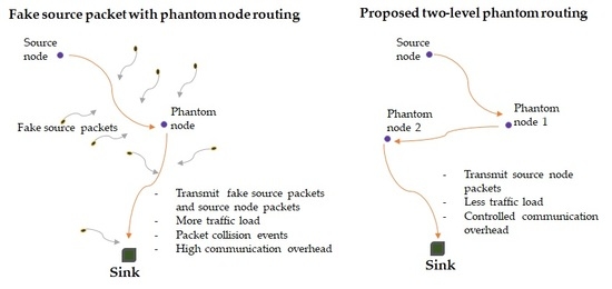
There exist several SLP routing protocols which integrate the phantom routing and fake packet routing strategies. Examples of the protocols include the tree-based diversionary routing (TreeR) [4] and the probabilistic source location privacy protection protocol (ProbR) [20]. The TreeR protocol achieves strong SLP protection by integrating many routing strategies. It employs phantom nodes which are located far away from the source node. It creates backbone routes which are directed to the network border with many diversionary routes. At the end of each diversionary route, fake packets are emitted periodically to obfuscate the adversary. The protocol incurs significant energy consumption, low PDR, and long EED due to the distribution of a large number of fake packets, some long routing paths, and long diversionary routes which diverge to the network border. The ProbR protocol considers transmission of two types of packets, fake packets and real packets as an efficient strategy to obfuscate an eavesdropping adversary. Real sources send packets to the sink node through phantom nodes. Concurrently, fake packets are transmitted to the sink node. The protocol achieves less effective SLP protection compared to the TreeR protocol. The TreeR and ProbR protocols have three main differences in their key features: (1) the TreeR employs fake source packets far away from the sink node, while ProbR employs fake source packets in the near-sink regions, (2) TreeR distributes a large amount of fake packets in the network while ProbR distributes only one fake packet at a time interval, and (3) TreeR distributes some fake packets near the phantom routes while ProbR locates the fake packet sources away from the phantom nodes. In this study, the performance of the TreeR and ProbR protocols were analyzed using five important performance metrics: safety period, attack success rate, energy consumption, PDR, and EED. Furthermore, two new phantom-based routing protocols, two-level phantom with a backbone route (PhaT), and two-level phantom with a pursue ring (PhaP) were proposed to address the limitations of TreeR and ProbR protocols, respectively. The proposed protocols introduced a new second level phantom node which was designed to provide a second level adversary confusion phase. A first level adversary confusion phase was provided by the first level phantom nodes which were adopted from the already existing phantom nodes in TreeR and ProbR. If an adversary embarked on back tracing the routing paths of the proposed protocols, it encountered two levels of adversary confusion phases. Consequently, the adversary made insignificant progress towards the source node and strong SLP protection was guaranteed.
The packet routing process of the proposed PhaP and PhaT protocols was done in three phases. Phase 1 involved the process of packet routing between the source node and the first level phantom node. The strategies for phase 1 in the PhaP and PhaT were adopted from the ProbR and TreeR protocols, respectively. Phase 2 involved the process of packet routing between the first level phantom node and the new second level phantom node. A new routing strategy was proposed for phase 2 to ensure second level phantom nodes were randomly and tactically positioned in the network. The random positions guaranteed that the routing paths were highly unpredictable to the adversaries, for strong SLP protection. Phase 2 may be considered as a replacement of the fake packet sources which exist in the TreeR and ProbR. Phase 3 involved the process of packet routing between the second level phantom node and the sink node. In PhaP, phase 3 was accomplished by utilizing a directed random-walk routing strategy. In PhaT, phase 3 was accomplished by utilizing a random backbone route which was generated between the sink node and a neighboring node of the second level phantom node. By removing the fake packets in the network, the proposed PhaP and PhaT protocols achieved controlled energy consumption, PDR, and EED. The PhaP protocol preserved stronger SLP protection than its contender ProbR protocol. The communication overhead in PhaT protocol was significantly improved as compared to its contender TreeR protocol. Furthermore, unlike the TreeR protocol, PhaT was more capable of controlling the communication overhead under varied network conditions such as varied source packet rate, varied network size, and varied source-sink distance. A summary of the performance features of the existing and proposed protocols is shown in Table 1.
The main contributions of this paper can be outlined as follows, (1) to propose two new routing protocols which employ a two-level phantom routing strategy with two adversary confusion phases, (2) to conduct a sequence of experiments to evaluate and compare the privacy performance of the proposed protocols with the existing TreeR and ProbR, (3) to demonstrate that the proposed protocols provide strong SLP protection with controlled communication overhead, and (4) to conduct a range of experiments to investigate the SLP protection, energy consumption, PDR, and EED performance of the protocols under varied network configurations.
The remainder of this paper is structured as follows: Section 2 provides a review of the literature on source location privacy routing protocols. Section 3 highlights the details of the network and adversary models. The proposed routing protocols are described in detail in Section 4. Performance analysis with the simulation results and discussions are presented in Section 5. In Section 6, the paper is concluded.
2. Related Work
The subject of SLP protection in WSNs has received widespread attention in the literature since it was first introduced in 2004 [2,11,21]. There exist many routing protocols for SLP protection [2,3,11]. In Reference [2], the SLP protection techniques were classified into the following categories, (1) phantom routing protocols, (2) fake packet injection protocols, (3) the multiple routing path protocols, (4) random walk routing, (5) hiding protocols, (6) ring routing protocols, (7) protocols based on the ring routing and the fake packet injection, (8) protocols based on the phantom routing and the fake packet injection, (9) data mule protocols, (10) cryptography and authentication protocols, (11) network encoding protocols, (12) directional communication protocols, and (13) the isolation protocols. In Reference [11], the routing protocols were classified into the following categories, (1) phantom node routing, (2) fake source routing, (3), intermediate node routing, (4) tree-based routing, and (5) the angle-based routing protocols. In Reference [21], the solutions for SLP protections were categorized into several strategies including (1) random walk routing, (2) fake source packet routing, (3) cyclic entrapment, and (4) geographic routing. In Reference [10], the solutions for providing the SLP protection were classified into eleven categories including (1) fake source packet routing, (2) random walk routing, (3) geographic routing, (4) cyclic entrapment, (5) separate path routing, (6) location anonymization, (7) cross-layer routing, (8) network coding, (9) delay, and (10) limiting the node detectability. In this study, we focus on phantom routing, fake source packet routing, and the protocols which adopt both phantom routing and fake source packet routing.
The phantom routing technique involves two main phases during the packet routing. In the first phase, packets are routed from the source node to a location where a phantom source is located through a random walk. At the phantom source, the packets are then forwarded to the sink node through flooding, single-path routing, or other strategies. The phantom routing strategy has been widely explored in the literature, and it has been adopted in many existing protocols. Examples of routing protocols which adopt phantom routing include the trace cost based source location privacy protection scheme [9], phantom walkabouts routing protocol [13], the phantom routing with locational angle [22], and the energy efficient privacy preserved routing algorithm [23]. Similarly, the phantom routing strategy is adopted in the multiple-phantom nodes routing scheme [24], the grid-based single phantom node and grid-based dual phantom node source location privacy protection schemes [25], the self-adjusting directed random walk approach [26], and the pseudo normal distribution-based phantom routing protocol [27]. The baseline phantom routing protocol offers low levels of SLP protection because it employs short and predictable routing paths. Adversaries can successfully perform back tracing attack on the short routing paths within a short time period. Furthermore, the phantom routing offers reduced levels of SLP protection when multiple source nodes exist in the network [28]. The fake source packet routing protocols involve the process of selecting a set of nodes in the WSN to act as fake sources and mimic the real sources. The fake sources and real sources send packets simultaneously to confuse the adversary. The fake source packet routing strategy has been adopted in many existing protocols including the dummy packet injection scheme [12], the dynamic fake sources-based algorithm [16], and the hybrid online dynamic single path routing algorithm [18]. Similarly, the fake source packet routing strategy is adopted in the forward random walk and bidirectional tree schemes [29], the fake network traffic-based scheme [30], the timed efficient source privacy preservation scheme [31], and the dummy uniform distribution, dummy adaptive distribution, and controlled dummy adaptive distribution protocols [32]. Often, the fake source packet routing protocols are criticized because of their high energy consumption, mainly because they rely on injecting a large number of fake packets to effectively protect the SLP. Furthermore, the protocols incur poor PDR and EED performance due to collisions between the packets.
There exist several protocol designs which adopt both the phantom routing and fake source packet routing strategies. The protocols include the tree-based diversionary routing [4], the enhanced source location privacy based on data dissemination protocol [7], the probabilistic source location privacy protection protocol [20], and the distributed protocol that combines fake source routing and phantom source routing [33]. The tree-based diversionary routing functions as follows; a phantom node is established and a backbone route is created based on the location of the phantom node. Then diversionary routes are created as branches of the backbone route. As many as possible diversionary routes are created to form tree-based routing paths. Fake packets are distributed at the end of each diversionary route to effectively obfuscate the adversary. During the back tracing attack, the adversary is tackled with two branch routes each time, thus the possibility of a successful back tracing attack is reduced to half. Thus, the protocol achieves strong SLP protection. The protocol incurs significant energy consumption as a result of the long routing paths and the distribution of a large number of fake packets in the network. Furthermore, the distribution of a large number of fake packets results in high probability of packet collision and packet loss events. Thus, the protocol incurs long end-to-end delay and low packet delivery ratio. The protocol may be unsuitable for delay sensitive applications or applications which require reliable packet delivery. In the probabilistic source location privacy protection protocol, phantom nodes are generated around the source node with the consideration of a visible area. A weight value is computed at each node to determine the next-hop candidates. Fake sources are generated around the sink node to send fake packets and confuse the adversary. The transmission involves two types of packets, the real packets from the source node and the fake packets from fake sources. To preserve the SLP, real packets from the source node are routed to a phantom node by utilizing directed random-walk routing strategy. One fake source transmits packets to the sink node at a fixed period of time. The protocol is less effective at protecting the SLP due to the fact that it utilizes only one fake packet source at a time period. A single fake packet source may not be very effective at confusing the adversary. Also, the fake source is isolated from the real packet source, and the real packet routes and fake packet routes are not exactly homogeneous, making it less difficult for the adversary to differentiate the two regions of fake source and real source. If the two regions are obvious to the adversary, the adversary can focus the tracing back attack on the real packet source region and increase the probability of a successful back tracing attack.
The enhanced source location privacy based on data dissemination protocol assumes a four quadrants square grid WSN with the sink node at the center of the grid. When a node wishes to send a packet to the sink node, the sink node generates a fake source and a phantom source depending on the location of the source node. A blast ring around the sink node contains nodes which are designed to flood packets inside the ring. When a blast node on the edge of the ring receives packets for forwarding, it starts flooding in a controlled manner. The protocol provides three levels of confusion to the adversary: fake node level, phantom node level, and the blast ring level. Limitations of the protocol includes high energy consumption when the size of the blast ring increases due to the widening of the area with flooding nodes. In the distributed protocol that combines fake source and phantom source routing, when a node wishes to transmit a packet to the sink node, it first floods a fake request packet into the network with a maximum hop count. Every node which receives the fake request packet checks their remaining energy levels and checks the number of times it has become a real source in the previous sessions. If a node has been a regular real source in the past, then it is disqualified from being a candidate fake source. If the energy level of the node is above a threshold value and it has not been a regular real source in recent sessions, then the node becomes a good candidate for fake source. The node computes a random number between 0 and 1. If the random number is greater than 0.5 then the node is selected as a fake source otherwise it ignores the request. When the node is selected as a fake source, it starts sending fake packets which are identical to real packets into the network. Subsequently, the source node selects a random node located at a distance away to act as a phantom node. After a phantom node is selected, the source node sends packets to the sink node through the selected phantom node. The main limitations of the protocol include high energy consumption due to the fake packet routing. Also, the protocol may incur long EED and low PDR due to packet collisions which may result from the simultaneous transmission of real packets and fake packets.
Although many routing strategies exist in the literature, a limited number of studies have addressed the limitations of the recently proposed fake packet routing protocols. Specifically, multilevel phantom node routing strategies have not been widely explored as an approach to address the limitations of fake packet routing protocols. In this study, we address the limitations of the fake packet routing protocols in References [4,20] by using two-level phantom routing protocols. In its baseline form, the phantom routing protocol is cost-effective. However, it offers low levels of SLP protection. We take advantage of the cost-effective phantom routing protocol. We propose two new two-level phantom routing protocols which offer high levels of SLP protection. The proposed protocols are PhaP and PhaT protocols. The PhaP protocol offers higher levels of SLP protection than the protocol in Reference [20]. Furthermore, the PhaP protocol achieves controlled energy consumption, PDR, and EED. In the near-sink region, the PhaP protocol achieves lower energy consumption than the protocol in Reference [20]. The PhaT protocol offers slightly lower levels of SLP protection than the protocol in Reference [4]. Nonetheless, the privacy protection of PhaT is effectively high. Comparing the communication overhead of the PhaT protocol and the protocol in Reference [4], the PhaT protocol achieves significantly lower energy consumption, significantly higher PDR, and lower EED.
3. Models
In this section, the design features of the proposed network model and adversary model are familiarized, and assumptions are presented.
3.1. Network Model
The network model assumed in this study is adopted from Reference [5]. The network model is a two-dimensional network domain which contains a set of sensor nodes and links. A wireless sensor node is a computing device enabled with a wireless interface, limited set of computational capabilities and has a unique identifier (ID). Three types of sensor nodes and sensor node capabilities exist in the network domain; sink node, source node and normal nodes. The sink node is a designated node for collecting data from the other nodes in the network. It also acts as an intermediate node between the WSN and the external world. The sink node has more capabilities than the other nodes. It has more memory capacity and more computational power. The main task of a source node is to sense an asset and forwarding the sensed data to the sink node by utilizing multi-hop communication. The functions of a normal node include relaying packets from source nodes to the sink node. All the sensor nodes in the network are stationary. Thus, the network topology does not change throughout the network lifetime. Communication from a node is modelled in a circular communication range which is centered at the node. All the sensor nodes are homogeneous and are designed to have the same communication range. The nodes which are in direct communication range with each other through 1-hop communication are assumed to be neighboring nodes and they can exchange data. Network is event-triggered, which means when a source node senses an asset, it can start sending packets to the sink node, periodically. When a node detects an asset within its monitoring area, it continues to sense the asset until the asset moves out of the area. When the asset moves to a new location, it activates another sensor node to become the new source node. When no asset is sensed, the nodes can follow a sleeping schedule. The packets which are transmitted between the sensor nodes are encrypted. Also, the packets contain source node ID but only the sink node can assume the ID as the asset location. The network functions in two phases. The first phase is the network configuration phase where network initialization and configurations are done. The second phase is the operational phase where packets are routed from the source node to the sink node by using the proposed routing protocols. During the network configuration phase, the network uses the network initialization process similar to References [3,8] as a technique for neighbor discovery and hop-count estimation of the nodes with respect to the sink node. The network uses the k-nearest neighbor tracking approach to track the assets.
Before the network initialization process, it is assumed that a network planner will have decided on the important network parameters such as the structure, size and configuration of the network regions. During the network initialization process, each sensor node is first loaded with a unique identifier (ID). Subsequently, the sink node acquires its location information through the use of a global positioning system (GPS). The sink node then broadcasts a beacon packet to all sensor nodes in the network and sets its hop counter to zero. The beacon packet contains information such as sink node ID, sink node position coordinates, and hop counter. Each node in the network receives the beacon packet, stores the hop counter value with a sender node ID, increments the hop counter by one, and rebroadcasts the beacon packet to its neighboring nodes. The hop counter number is used to indicate the hop distance between the sensor nodes and the sink node. The broadcasting of the beacon packet ensures each node acquires information and knowledge about its neighboring nodes and its location with regard to the sink node. If a sensor node receives multiple beacon packets, it stores the minimum hop count in its buffer and deletes other hop counter information. After that, each sensor node computes a list of its neighboring nodes. Each node notifies its hop distance to the sink node. At the same time, the network planner may identify the network regions and assign the role of the sensor nodes according to their location in the network. Since all the sensor nodes are assumed to be stationary, the location and neighborhood information of all nodes remain constant throughout the network lifetime.
3.2. Adversary Model
The adversary model assumed in this study is adopted from Reference [5]. It is assumed that the adversary is well equipped and it has adequate resources such as computation capabilities, memory and unlimited power. It is equipped with antenna and spectrum analyzers to enable it to monitor the communication between sensor nodes when it is within a certain detection range. It is capable of analyzing the traffic pattern. The adversary is mobile, it is initially located in the locality of the sink node to listen for arriving packets. The benefit of initial location at the sink node is to increase the probability that the adversary will overhear packets due to the large volume of packet traffic at the destination sink node. When a packet arrives at the sink node, the eavesdropping adversary will overhear and start the back tracing attack by moving 1 hop towards the source node until it locates the source node. According to Kerckhoff’s principle, the adversary is aware of the routing strategy which is used in the network and it assumes the transmission range similar to that of sensor nodes. When the adversary detects a packet, it can analyze the angle of arrival of the signal and the received signal strength to identify the immediate sender node. It then performs back tracing attack by moving to the immediate sender node location without delay. Once at the immediate sender node, the adversary continues to analyze the traffic pattern between the node and its neighboring nodes. It targets to capture information such as sender node ID, packet type, and sequence number. It continues to analyze the traffic pattern and back trace the packet routes until it arrives at the source node location to locate the asset. The adversary is capable of capturing all packets within its detection range and it never fails to detect a packet. It performs passive attacks and avoids interfering with the functioning of the nodes in network. To avoid getting noticed by the network administrators, adversary does not interfere with the packets transmission and does not destroy the sensor node equipment. The adversary is a cautious adversary. It uses its computational power to limit its waiting time at any immediate sender node. At an immediate sender node, it observes a waiting timer and if the timer expires, the adversary will roll back to its previous immediate sender node and resume the traffic analysis and packet detection process. In addition, the adversary stores the information of all the visited immediate sender nodes to evade revisiting the nodes. By doing do, it reduces the probability of getting trapped in a loop.
4. Proposed Routing Protocols
Two new routing protocols are proposed, namely, the two-level phantom with a pursue ring (PhaP) and two-level phantom with a backbone route (PhaT) protocols. The proposed PhaP and PhaT protocols can be considered as modified versions of the probabilistic source location privacy protection routing protocol (ProbR) [20] and the tree-based diversionary routing protocol (TreeR) [4], respectively. The two main goals of the proposed protocols are to: (1) provide strong SLP protection throughout the WSN domain, and (2) control the communication overhead by removing the fake packet traffic in the network. The PhaP and PhaT protocols introduce a two-level phantom routing strategy. In the strategy, packet routing is done in three phases. In phase 1, packets are routed from the source node to the first level phantom node. The routing strategy for phase 1 in the PhaP and PhaT are adopted from the ProbR and TreeR protocols, respectively. Phase 2 involves the process of packet routing from the first level phantom node to the new second level phantom node using two new routing strategies. The new routing strategies are explained in details in the next sub-sections. Phase 3 involves the process of packet routing from the second level phantom node to the sink node. In PhaP, phase 3 is accomplished by utilizing a directed random-walk strategy. In PhaT, phase 3 is accomplished by utilizing a random backbone route which is generated between the sink node and a neighboring node of the the second level phantom node. A new backbone routing strategy is proposed. The key differences between the routing strategies of the proposed and existing protocols are highlighted in Table 2. For both PhaP and PhaT protocols, the two-level phantom routing strategy is designed to provide two adversary confusion phases. The first level phantom node provides first level adversary confusion phase while the second level phantom node provides second level adversary confusion phase. If an adversary embarks on back tracing the routing paths, it encounters two levels of adversary confusion phases. Thus, strong SLP protection is guaranteed. The proposed PhaP and PhaT routing algorithms are summarized in Algorithms 1 and 2, respectively.
4.1. Proposed Two-Level Phantom with a Pursue Ring Protocol (PhaP)
To facilitate the discussions of the proposed PhaP protocol, Table 3 shows the notations used in the protocol description.
4.1.1. PHASE 0: Network Configuration
For proper functioning of the PhaP protocol, a pursue ring (Pring) is computed during the network configuration phase, after the network initialization process. The network initialization process is explained in Section 3 above. The Pring is computed during network configuration phase to minimize delay during packet routing. To begin the Pring computation process, an X-Y coordinate is generated at the sink node location and two distances are defined, the distance from sink node to the inner ring of the Pring (dPin) and the distance from sink node to the outer ring of the Pring (dPout). Distance between any two points in the network is calculated using the Euclidian distance equation. For example, the distance between point U at (xU, yU) and point V at (xV, yV) is calculated as: . A ring with dPin and dPout is generated. The configuration of the Pring regions in the WSN domain is shown in Figure 1. All sensor nodes which are located in the Pring are recoded in a list of candidate second level phantom nodes (PNsec). To diversify the routing paths, the Pring is divided into four parts: north-east region of Pring (PrNE), south-east region of Pring (PrSE), north-west region of Pring (PrNW), and south-west region of Pring (PrSW). The flowchart for the Pring computation process is shown in Figure 2. To specify the Pring regions, the inclination angle, θ, of all the sensor nodes in the Pring is computed. The θ is the angle formed between the X-axis and the imaginary line connecting the sink node and the node which is computing the θ as shown in Figure 3. The computation of θ is based on three parameters: the distance between the sensor node and the sink node, the distance between the sensor node and the meeting point on the X-axis, and the position coordinates of the sink node, the sensor node, and the meeting point on the X-axis. As an example in Figure 3, if node C which is located at (xC, yC) wants to compute the inclination angle θC, the line connecting node C and the X-axis meet at point L with coordinates (xL, yL). The sink node is at (x0, y0). Then the distance, dSL, between the sink node and point L is calculated as: . Similarly, the distance, dSC, between the sink node and node C is calculated as: . Then, the inclination angle θC is computed as . The sensor nodes with θ in the range 0° ≤ θ < π/2, π/2 ≤ θ <π, π ≤ θ < 3π/2, and 3π/2 ≤ θ < 2π are assigned in PrNE, PrNW, PrSW, and PrSE, respectively.
4.1.2. PHASE 1: Selection of a First Level Phantom Node (PNfst) and Packet Routing from Source Node to PNfst
After the Pring is configured, the network is ready for packet routing. The proposed PhaP routing algorithm is summarized in Algorithm 1. The packet routing process is done in three phases. Phase 1 routing is activated by the source node when the source node detects an asset. The source node selects a random first level phantom node (PNfst) using similar phantom node selection algorithm as in ProbR. After PNfst is selected, it sends packet to the PNfst using a directed random-walk routing strategy. The directed random-walk routing strategy involves a process of next-hop node selection at every packet forwarding instance. The forwarding node computes a set of neighboring nodes with a shorter hop distance to the destination node than the forwarding node itself. Then it randomly selects one neighboring node from the set as the next-hop node. The next-hop node becomes the forwarding node and forwards the packet. For easy of understanding, the group of neighboring nodes with shorter hop distance to the destination node is termed as SDRN, in Algorithms 1 and 2. Also, the selected next-hop node from the SDRN is termed as DRN and the destination nodes are termed as target node. At the source node, the destination node is the selected PNfst.
4.1.3. PHASE 2: Selection of PNsec and Packet Routing from PNfst to PNsec
After the PNfst receives a packet from PNfst, it sets a bias threshold value, TP. Then it generates a random number, RN, between [0, 1]. The RN and TP values are compared. Depending on the comparison results, PNfst selects a random PNsec according to Table 4. The PNsec selection process is highly dependent on the location of the PNfst with respect to the sink node. The PNfst may be located on the east or west side of the sink node according to the Y-axis. After the PNsec is selected, PNfst forwards the packet to the randomly selected PNsec using the directed random-walk routing strategy. To guarantee high path diversity for successive packets, new PNfst and PNsec are selected for each packet transmission.
4.1.4. PHASE 3: Packet Routing from PNsec to Sink Node
After packets arrive at the PNsec, they are forwarded to the sink node using the directed random-walk routing strategy. At the PNsec, the destination node is the sink node as shown in Algorithm 1.
| Algorithm 1. Proposed algorithm for PhaP protocol | |
| Phase 0: Network configuration | |
| 1: | sink_node_location = (0,0) |
| 2: | network initialization using same algorithm as in Reference [3] |
| 3: | generate X–Y coordinate centered at the sink_node |
| 4: | create Pring according to Figure 1 |
| 5: | compute θ according to Figure 3 |
| 6: | if (0° ≤ θ < π/2) |
| 7: | assign node into PrNE |
| 8: | else if (π/2 ≤ θ < π) |
| 9: | assign node into PrNW |
| 10: | else if (π ≤ θ < 3π/2) |
| 11: | assign node into PrSW |
| 12: | else if (3π/2 ≤ θ < 2π) |
| 13: | assign node into PrSE |
| 14: | end if |
| Phase 1: Selection of PNfst and packet routing from source node to PNfst | |
| 15: | sensor node detect asset, becomes source_node |
| 16: | source_node select PNfst using same algorithm as in Reference [20] |
| 17: | Packet routing (source_node, PNfst) // source node send packet to PNfst using directed random-walk routing |
| Phase 2: Selection of PNsec and packet routing from PNfst to PNsec | |
| 18: | bias_threshold = TP |
| 19: | PNfst generate RN between [0, 1] |
| 20: | if (X-coordinate_of_PNfst < X-coordinate_of_sink) |
| 21: | if (RN < TP) |
| 22: | select PNsec from PrNW |
| 23: | else |
| 24: | select PNsec from PrSE |
| 25: | end if |
| 26: | else if (X-coordinate_of_PNfst ≥ X-coordinate_of_sink) |
| 27: | if (RN < TP) |
| 28: | select PNsec from PrNE |
| 29: | else |
| 30: | select PNsec from PrSW |
| 31: | end if |
| 32: | end if |
| 33: | Packet routing (PNfst, PNsec) // PNfst send packet to PNsec using directed random-walk routing |
| Phase 3: Packet routing from PNsec to sink | |
| 34: | Packet routing (PNsec, sink) // PNsec send packet to sink using directed random-walk routing |
| 35: | function Packet routing (sender_node, target_node) // directed random-walk routing |
| 36: | sender_node generate SDRN |
| 37: | sender_node select DRN |
| 38: | while (DRN != target_node) |
| 39: | sender_node = DRN |
| 40: | sender_node generate SDRN |
| 41: | sender_node select DRN |
| 42: | end while |
| 43: | end function |
4.2. Proposed Two-Level Phantom with a Backbone Route Protocol (PhaT)
To facilitate the discussions of the proposed PhaT protocol, Table 5 shows the notations used in the protocol description.
4.2.1. PHASE 0: Network Configuration
In the PhaT protocol, it is assumed that the near network border region is defined during the network configuration phase. Distance between any two points in the network is computed using the Euclidian distance equation. As an example, the distance between point J at (xJ, yJ) and point B which is located on the network border at (xB, yB) is calculated as: . The outer boundary of the near network border region is the network border. The inner boundary of the near network border region is defined at distance dNB from the network border. Therefore, the near network border region is the region within distance dNB from the network border. All sensor nodes which are located within distance dNB from the network border are identified as nodes in the near network border regions (NNB). To compute a distance from location of a sensor node to the network border (dSB), the location coordinates of the sensor node (xS, yS) are used. For any sensor node, if dSB ≤ dNB, the sensor node is added in the list of NNB. All NNB may be selected as a first level phantom node (epN) during packet routing. The algorithm for PhaT protocol is summarized in Algorithm 2. The last task in the network configuration phase is the process where each NNB computes a list of candidate second level phantom nodes (npN). For each NNB, an npN is a sensor node which is located at hop distance, dP, away. For example, if node N20 is in the list of NNB, and dP is specified as 4 hops, then N20 will compute a list of all sensor nodes which are located 4 hops away. As an example, N20 may compute a list containing nodes N8, N30, N14, and N57. During packet routing, if N20 is selected as epN, then it may select N8, N30, N14, or N57 as the second level phantom node (npN). Figure 4 shows the configuration of sensor nodes in the proposed PhaT protocol.
The location configuration of the candidate npNs is guarded by a restricted region, RR, around the epN. RR is defined by radius of hop distance dH from epN. dH is used to ensure a safe distance between epN and npN. All the neighboring nodes of epN are located inside the RR. The distances dH and dP have a relationship which satisfy the equation . While dH specifies the sensor nodes which are restricted from becoming npN, dP is used to specify the sensor nodes which are good candidate for npNs. The npN are located outside the RR to ensure the epN and npN are not neighboring nodes. Longer dP increases the distance between the epN and npN, increases the complexity for the adversary back tracing attack, and improves the SLP protection. To guarantee routing paths with high path diversity, two unique regions of npNs are defined. The regions are north of epN (northR) and south of epN (southR). If a node is a candidate npN with Y-coordinate greater than the Y-coordinate of the epN, it is identified as a candidate npN in northR. Otherwise, if a node is a candidate npN with Y-coordinate less than or equal to the Y-coordinate of the epN, it is identified as a candidate npN in southR.
The protocol employs the phantom nodes in the near network border regions to ensure effectively long and diversified routing paths. To control the communication overhead of the protocol, the near network border regions must be configured according to the network topology to ensure the routing paths are not excessively long. If the network size is very large, the distance between phantom nodes and the sink node may be excessively long and the protocol may incur high communication overhead. To route packets, the protocol operates in three phases as shown in Algorithm 2.
| Algorithm 2. Proposed algorithm for the PhaT protocol | |
| Phase 0: Network configuration | |
| 1: | network initialization using the same algorithm as in Reference [3] |
| 2: | |
| 3: | |
| 4: | ifdSB ≤ dNB |
| 5: | add sensor node to list of epN |
| 6: | each epN generate a list of npN |
| 7: | if (Y-coordinate_of_npN > Y-coordinate_of_epN) |
| 8: | assign npN into northR |
| 9: | else |
| 10: | assign npN into southR |
| 11: | end if |
| 12: | end if |
| Phase 1: Selection of epN and packet routing from source node to epN | |
| 13: | sensor node detect asset, becomes source_node |
| 14: | source_node select epN from list of epN using the same algorithm as in Reference [4] |
| 15: | Packet routing (source_node, epN) // source node send packet to epN using directed random-walk routing |
| Phase 2: Selection of npN and packet routing from epN to npN | |
| 16: | bias_threshold = T |
| 17: | generate SF between [0, 1] |
| 18: | if (SF > T) |
| 19: | select npN from northR |
| 20: | else |
| 21: | select npN from southR |
| 22: | end if |
| 23: | Packet routing (epN, npN) // epN send packet to npN using directed random-walk routing |
| Phase 3: Selection of BN and packet routing from npN to sink node | |
| 24: | npN select BN |
| 25: | BN select NWSD |
| 26: | while (NWSD != sink) |
| 27: | FWN = NWSD |
| 28: | FWN select NWSD |
| 29: | end while |
| 30: | npN send packet to BN and BN forward packet to sink using shortest path routing |
| 31: | function PacketRouting (send_node, target_node) // directed random-walk routing strategy |
| 32: | send_node generate SDRN |
| 33: | send_node select DRN |
| 34: | while (DRN != target_node) |
| 35: | send_node = DRN |
| 36: | send_node generate SDRN |
| 37: | send_node select DRN |
| 38: | end while |
| 39: | end function |
4.2.2. PHASE 2: Selection of npN and Packet Routing from epN to npN
When the epN receives the packet from the source node, it activates the npN selection process to select one npN from the list of npN. A random selection factor (SF) is generated by the epN. The SF is distributed between [0, 1]. If SF > T, npN is randomly selected from the candidate npNs in northR. Otherwise, npN is selected from the candidate npNs in southR. After npN is selected, phase 2 routing is done. The epN forwards the packet to the npN using the directed random-walk routing strategy.
4.2.3. PHASE 3: Selection of BN and Packet Routing from npN to Sink Node
After the npN receives the packet, it activates the process to select an initial backbone route node (BN) which is used to create a backbone route to the sink node. The npN selects a neighboring node with the longest hop distance to the sink node as the BN. As an example, in Figure 4, if npN3 receives a packet from epN, BN9 may be selected as the BN. If multiple nodes have equal longest hop distance to the sink node, one of the nodes is randomly selected. After the BN is selected, phase 3 routing is done. The npN forwards the packet to the BN and the BN forwards the packet to the sink node through a backbone route. The backbone route employs the shortest path routing strategy. At each forwarding node (FWN), the node with the shortest hop distance to the sink node (NWSD) is selected as the next-hop node. When the NWSD is the sink node, the packet is delivered at the sink node. The shortest path routing strategy is employed to ensure controlled communication overhead. New epN, npN, SF, and backbone route are computed for each successive packet to guarantee high path diversity and strong SLP protection.
5. Performance Analysis
5.1. Simulation Environment
Performance analysis to evaluate the performance of the proposed protocols was done using MATLAB simulation environment. A WSN domain of size 2000 × 2000 m2 was simulated. For good coverage in the network, 2500 nodes were randomly distributed. Sink node was the destination for all the packet transmissions. The location of the sink node was assumed at the center of the network. The sensor node sensing range was set to 30 m to guarantee multi-hop communications between source nodes and sink node. The k-nearest neighbors tracking approach was employed to monitor the network domain. The network model is explained in details in Section 3 above. A total of five protocols were included in the analysis: the ProbR, PhaP, TreeR, PhaT, and the phantom single-path routing (Pha). The Pha protocol was included in the analysis as a representative protocol for the traditional SLP routing protocols, for comparative analysis. The network configuration for the PhaP protocol was done according to Figure 1. The network parameters were configured as follows: , , and . For PhaT protocol, , , , and . A cautious adversary was deployed with initial location around the sink node to ensure maximum probability of packet capture. Adversary detection range was set to 30 m similar to sensor node sensing range to guarantee that the adversary performs hop-by-hop back tracing attack. The waiting timer for the adversary was set to four source packets. The adversary model is explained in details in Section 3 above. Only real packets were transmitted in the PhaP and PhaT protocols. In the ProbR and TreeR, real packets and fake source packets were transmitted simultaneously. The simulation was run for 500 iterations and average values were considered. The network simulation parameters are summarized in Table 6. The performance metrics used in the analysis are explained in the next sub-section.
5.2. Performance Metrics
The following performance metrics were used for analysis:
- (1)
- Safety Period (SP): the same as in Reference [3], safety period can be defined in multiple ways: (i) the time required for an adversary to successfully back trace and capture the asset, (ii) the number of packets successfully delivered to the destination sink node before the adversary locates the source node, or, (iii) the maximum duration of time the monitored asset will be at a given location before it moves to a new location. The first definition is assumed in this study. Safety period is used to measure the privacy performance of the protocols. Longer safety periods provide stronger SLP protection. To evaluate the SLP performance, the following expression was assumed
- (2)
- Attack success rate (ASR): the measure of the rate of source node traceability when an eavesdropping adversary is back tracing against a SLP routing protocol. It is computed by counting the number of successful adversary attempts [8]. ASR has an inversely proportional relationship with the safety period. When a protocol achieves a long safety period and high privacy, the ASR is low. To evaluate the ASR of the adversary, the following expression was assumed
- (3)
- Energy consumption: the energy consumed by the sensor nodes for transmitting and receiving packets as shown in Equations (1,2). The energy consumption model was adopted from References [3,4,5,7]. To transmit an l-bit packet to a transmission distance d, transmission energy, Etrans, and receive energy, Erec, follow Equations (1,2), respectively. According to the model, energy consumption for packet transmission is an exponential function of d. Eloss represents the transmitting circuit loss. Two loss models are applied, the free space (d2 power loss) and the multi-path fading (d4 power loss) channel models. If the transmission distance between sensor nodes is less than the threshold d0, the power amplifier loss is based on free-space model. Otherwise if the transmission distance is equal or greater than the threshold d0, the multi-path attenuation model is used. The threshold distance, d0, is computed according to Equation (3). Efs and Eamp are the energy required by power amplification in the two power loss models. Table 7 shows the energy consumption model parameters as adopted from References [3,4,5,7].
- (4)
- Packet delivery ratio (PDR): the ratio between the total numbers of packets successfully delivered to the destination sink node and the number of packets transmitted by the source nodes. To evaluate the PDR performance, Equation (4) was adopted from References [34,35].where PRec is the total number of data packets successfully received by the destination sink node. PTrans is the number of packets transmitted by the source nodes. n is the number of source nodes.
- (5)
- End-to-end delay (EED): the time taken for a packet to be transmitted across the network from a source node to the destination sink node. To evaluate the EED, Equation (5) was assumed, as adopted from [34,35].where TRec is the time when data packet is received by the sink node. TTrans is the time when each data packet is transmitted by a source node. PRec is the total number of data packets received at the destination sink node.
5.3. Simulation Results and Discussions
Two experiment scenarios, experiment scenarios (a) and experiment scenarios (b), were done for performance analysis of safety period, energy consumption, packet delivery ratio, and end-to-end delay. In the scenarios (a), the performance was observed under fixed source packet rate of 1 packet/second against varied source-sink distance. The source-sink distance was varied between 10 and 70 hops. In scenarios (b), performance was observed under fixed source-sink distance against varied source packet generation rate. The source packet generation rate was varied from 1 to 7 packet/second. For the analysis of attack success rate, three experiment scenarios were done. In scenario (a), the attack success rate was observed against varied number of sensor nodes in the network. In scenario (b), the attack success rate was observed at varied network size. In scenario (c), the attack success rate was observed against varied adversary detection range.
Figure 5 shows the privacy performance of the protocols. The figure shows that the TreeR protocol achieves very strong SLP protection. The TreeR achieves longer safety period by integrating many routing techniques. It employs phantom nodes located far away from the source node. It also employs significantly long backbone routes with many diversionary routes. At the end of each diversionary route, fake packets are emitted periodically. As a result, the eavesdropping adversary is effectively obfuscated and long safety period is guaranteed. However, the use of long backbone routes, diversionary routing paths which diverge to the network border regions, and the distribution of fake packet traffic at the end of each diversionary route introduce very high communication overhead as shown in the next paragraphs. The figure also shows that the proposed PhaT protocol achieves relatively short safety period compared to the TreeR protocol. However, compared to the traditional Pha protocol, the PhaT protocol offers significantly longer safety period. For example, at 60 hops from the sink node, the safety period of the PhaT is approximately 4 times higher than Pha protocol. Since PhaT can achieve approximately 4 times higher safety period than the Pha protocol, we consider the level of SLP protection for PhaT to be effectively strong. Also shown in the Figure 5a, the proposed PhaP protocol achieves significantly longer safety period than the existing ProbR protocol. The ProbR protocol achieves a relatively short safety period because the fake packet source is located away from the real source node, on the opposite side of the real source node. Also, the real packet routes and fake packet routes are not exactly homogeneous due to the location of the fake packet sources being in the near-sink region. The fake packet routes are relatively short. As a result, it has a small effect on the privacy protection. After sometime of traffic analysis attack, adversary can predict the real packet routes and perform a more focused back tracing attack to improve its attack success rate. Furthermore, the ProbR protocol distributes only one fake packet at a time. As a result, the adversary is not effectively distracted from the real packet routes and short safety period is achieved by the ProbR protocol. The safety period of Pha protocol is significantly lower because the protocol employs a simple routing algorithm with short and fixed routes. The adversary is capable of successfully back tracing the routing paths of the Pha within a short time. For all the protocols, the privacy performance improves with the increase in source-sink distance because the adversary back tracing attack becomes more complicated with longer routing paths. Figure 5b shows the privacy performance of the protocols at a source-sink distance of 40 hops against varied source packet generation rate. The protocols offer lower safety period as the source packet rate increases. The main reason for the reduced safety period is that, as more packets are sent in the network, the probability that the cautious adversary will capture successive packets within the specified waiting timer is increased. At higher data rates, the cautious adversary is capable of capturing enough number of successive packets to allow it to make a successful back tracing attack and capture the asset. Therefore, the level of SLP protection is reduced.
Figure 6 shows the attack success rate (ASR) of the adversary against the analyzed protocols. In the analysis, the source packet generation rate was 1 packet/second, the adversary trace time was 900 source packets, and the source-sink distance was fixed at 50 hops. For the results in Figure 6a, the ASR was observed against varied number of sensor nodes in the network. The number of sensor nodes was varied between 2500 and 4000 nodes. The figure shows that the ASR of all the protocols tend to decrease with the increase in the number of sensor nodes in the network. However, for the proposed protocols, the ASR decreases at a slightly higher rate. This means that, the SLP protection in the proposed protocols increases at a higher rate that in the other protocols. The main reason for the increased SLP protection with the increase in node density is that, when the number of nodes in the network increases, the number of neighboring nodes and candidate phantom nodes also increase. As an example, in PhaP protocol, when the node density increases it also increases the probability of a greater number of nodes in the Pring. Therefore, the number of candidate PNsec for each successive packet also increases. As a result, there is a higher probability that a different PNsec is selected for each successive packet and the routing paths becomes less predictable to the eavesdropping adversary. Also, the number of random routing paths increases with the increase in number of neighboring nodes of the PNfst and PNsec. As an example, if a source node has w neighboring nodes with shorter hop distance to PNfst, the probability of the source node selecting a particular neighboring node as the next-hop node during the directed random-walk is 1/w. If PNfst has k neighboring nodes with shorter hop distance to PNsec, the probability of PNfst selecting a particular neighboring node as the next-hop node during the directed random-walk is 1/k. If PNsec has v neighboring nodes with shorter hop distance to sink, the probability of PNsec selecting a particular neighboring node as the next-hop node during the directed random-walk is 1/v. Overall, there can be up to random routes between the source node and the sink node. That is, . It is therefore evident that the SLP protection will increase with the increase in node density. As a result, ASR decreases with the increase in node density. This effect is similar in the PhaT protocol. The ProbR protocol employs only one phantom node and one fake packet source in the near-sink region. As a result, the increase in node density has a small effect on limiting the ASR. The TreeR depends highly on the fake packet routes to obfuscate the adversary. Since the number of diversionary routes remained the same, obfuscation of the adversary on the backbone route does not improve very much with the increase in node density. As a result, ASR decreases at a slow rate. The Pha protocol selects the shortest paths which may become fixed, as a result, the increase in node density has little effect on the ability of the protocol to limit the ASR.
Figure 6b shows the ASR of the adversary against varied network size. The network has a square structure. For analysis, we use the term “Length” which means the length or width of the network. In the experiments, the length was varied between 2000 and 3500 m. In the figure, it shows that the ASR against the Pha, ProbR, and PhaP protocols has insignificant change as the length increases. The main reason for the insignificant change is that the routing paths of the protocols are directed towards the sink node. Since the source-sink distance remained the same and the phantom node selection criteria did not change, the change in the network size had no significant impact on the performance of protocols. In the PhaT protocol, the ASR decreases significantly with the increase in length. The main reason for the improved privacy performance as length increases is that, since the location of the sink node is constant at the center of the network, then the distance between the sink node and phantom nodes increases with the increase in length. This is mainly because the phantom nodes are located in the near network border regions. Also, since the source-sink distance was fixed at 50 hops, the distance between the source node and phantom nodes increase with the increase in length. As a result, the routing paths become longer and the directed random-walk routing strategy becomes more obfuscating to the adversary. Consequently, the adversary takes longer time to back trace the packet routes, makes insignificant progress towards the source node, and the ASR is limited. However, for the proposed PhaT protocol, it is important to control the length. If the length is too long, it may lead to excessively long routing paths which incur high communication overhead. In the TreeR protocol, when the intermediate node is kept at a fixed location, it is possible to increase the length of the diversionary routes as the network size increase. As a result, the obfuscation ability of the protocol is increased. When the adversary is misled into back tracing the diversionary routes which become longer with the increase in length, the adversary may be misled into regions further away from the source node. Hence, the ASR is reduced.
Figure 6c shows the ASR of the adversary against adversary detection range. The adversary detection range was varied between 30 and 90 m. The sensor node sensing range was fixed at 30 m. The figure shows that the ASR increases with the increase in adversary detection range. This is mainly due to the fact that adversary becomes more powerful when it has a longer detection range. The traffic analysis attacks become less complex when the adversary can detect a packet sent from a sensor node which is more than 1 hop away. The figure shows that, when a source node is 50 hops away from the sink node, at a trace time of 900 source packets, an adversary with 60 m detection range can achieve up to 100% ASR against the Pha protocol. An adversary with 90 m detection range can achieve up to 90% ASR against the ProbR protocol and up to 65% ASR against the PhaP protocol. For PhaT and TreeR protocols, an adversary with 90 m detection range can achieve less than 55% ASR. These results establish that, amongst all the analyzed protocols, the PhaT and TreeR protocols have the strongest SLP protection and when the adversary has 30 m detection range, the protocols are capable of limiting the adversary ASR to less than 25%.
Figure 7 shows the energy consumption performance of the protocols. In the energy consumption analysis, 15 experiment scenarios were assumed, each scenario with a different source node location. Each scenario involved a transmission of 1000 packets from a source node to the sink node. After all the packets were received at the destination sink node, for each scenario, the average energy consumption per sensor node was computed according to Equations (1) and (2). For both TreeR and ProbR protocols, real packets and fake packets were transmitted simultaneously. Figure 7a shows the average total energy consumption per sensor node for sensor nodes at different locations. The figure shows the energy consumption of TreeR protocol is significantly high. The high energy consumption is due to the integration of many routing techniques. The backbone routes which divert to the network border cause the protocol to generate long routing paths. Also the multiple diversionary routes which act as branches for the backbone routes distribute a large amount of fake packets. Fake packets are also distributed along the phantom route. As a result, the sensor nodes incur exhaustive energy consumption. Furthermore, multiple fake packets are transmitted for each real packet transmission. As shown in Equations (1) and (2), each hop involves consumption of transmit and receive energy. As a result, more energy is consumed for each real packet transmission. Moreover, the distribution of fake packets in the network increases the probability of packet collision events which result in packet retransmission incidents. Hence, higher energy consumption is incurred by the TreeR protocol. The proposed PhaT has significantly lower energy consumption than the TreeR protocol mainly because while the PhaT protocol employs a single route for each packet transmission, the TreeR protocol employs multiple routes which include a route for real packet transmission and multiple diversionary routes for fake packets transmission. Both TreeR and PhaT protocols employ backbone route near the sink region to minimize the energy consumption in the region. The energy consumption of PhaT is higher than in the ProbR, PhaP, and Pha protocols. The main reason for the high energy consumption is that, PhaT locates the phantom nodes in the network border regions which results in longer and highly diversified routing paths.
In the near-sink region, ProbR protocol incurs higher energy consumption than the proposed PhaP because ProbR transmits multiple packets for each event packet. A fake source packet is transmitted with every real packet transmission. Sensor nodes in the near-sink region experience exhaustive energy consumption due to the big load of packet forwarding. The sensor nodes not only transmit their own packets to the sink node, they also forward packets originating from the sensor nodes in the away from sink regions. The PhaP protocol ensures the energy consumption of the sensor nodes in the near-sink region is minimized. In the away from the sink regions, PhaP and Prob incur same amount of energy consumption because the protocols employ a similar phantom node routing strategy in the away from the sink regions. The energy consumption of the Pha protocol is significantly lower because the protocol employs a simple routing algorithm with short and fixed routes. Figure 7b shows the energy consumption of sensor nodes at 600 m from the sink node, against varied source packet generation rate. The energy consumption of the sensor nodes increases with the increase in source packet generation rate. At higher packet rates, more packet traffic is generated in the network. Consequently, the sensor nodes consume more energy to transmit the packets. The energy consumption of TreeR protocol increases at a faster rate because more packet collision events occur due to the transmission of both, real packet and fake packets. More packet collision events result in packet loss and packet retransmission events. As a result, the energy consumption of the sensor nodes is increased.
Figure 8 shows the packet delivery ratio (PDR) performance of the protocols. Figure 8a shows the PDR performance of the protocols at a fixed source packet rate. The analysis included source nodes at different source-sink distances. 100 packets were transmitted from each source node to the sink node with a fixed source packet generation rate of 1 packet/second. Average values for PDR were found according to Equation (4). The figure shows that PDR of all the protocols decreases with the increase in source-sink distance. This is due to the fact that as the distance between the source node and sink node increases, more hops are included in the transmission and the probability of packet loss increases. Therefore, the PDR performance is affected. The figure shows that the TreeR protocol incurs low PDR. The low PDR performance of TreeR is due to the integration of many routing strategies. The use of phantom nodes, backbone routes, and diversionary routes result in routing paths which have high probability of packet loss events and low PDR. Furthermore, the distribution of fake packets in the network results in high probability of packet collision events and low PDR is achieved. The proposed PhaT protocol achieves higher PDR than the TreeR protocol because it incurs few packet collision and packet loss events due to the absence of fake packet distribution. The ProbR protocol achieves higher PDR than the TreeR protocol because it employs shorter routing paths with only one fake packet source at a time period. The ProbR and PhaP protocols have comparable PDR performance because they both employ phantom node routing with routing paths which are directed towards the sink node. The fake packet sources in the ProbR are located far away from the real sources. Consequently, the fake packets incur less significant effect on the PDR of the protocol. The PDR of the Pha protocol is significantly high because the protocol employs a simple routing algorithm with short and fixed routing paths. The short and fixed routing paths incur few events of packet loss and packet collision. Figure 8b shows the PDR performance of the protocols at a fixed source-sink distance of 40 hops. The experiment scenarios included multiple source nodes. 100 packets were sent from each source node to the sink node at varied source packet rate from 1 to 7 packet/second. The figure shows that PDR of all the protocols decreases with the increase in source packet rate. When more packets are generated per second, the probability of packet collision and packet loss is increased and PDR is affected. The TreeR protocol incurs the worst PDR performance at high source packet rates due to the increasing number of packet collision events between the real and fake packets.
Figure 9 shows the end-to-end (EED) performance of the protocols. Figure 9a shows the EED performance of the protocols at different source-sink distances. Investigations were done for multiple source nodes at different source-sink distances. 100 packets were sent from each source node to the sink node with a fixed source packet generation rate of 1 packet/second. Average values for EED were found according to Equation (5). The figure shows that the EED of the protocols tend to increase with the increase in the source-sink distance. This is due to the fact that as the distance between the source node and sink node increases, the number of packet forwarding events (hops) also increases. Each hop incurs some EED. Hence, the overall EDD is increased. Furthermore, longer routing paths have a higher probability of packet loss and packet retransmission events which have negative effect on the EED performance. The TreeR and PhaT protocols employ long routing paths. Consequently, the EED for the TreeR and PhaT protocols is long. The location of phantom nodes in the ProbR and PhaP protocols guarantee relatively short routing paths with better EED performance than the TreeR and PhaT protocols. The fake source packets in ProbR are located far away from the real source node. As a result, the fake packets have less significant effect on the EED performance of the protocol. The Pha protocol has significantly low EED because the protocol employs a simple routing algorithm with short and fixed routing paths. Figure 9a also shows the impact of adding a second level phantom node routing on the EED of the PhaP and PhaT protocols. The PhaP has a slightly longer EED than ProbR. The increase in EED is controlled by the strategic location of the Pring which guarantees that the directed random-walk routing is directed towards the sink node. The PhaT has considerably lower EED than the TreeR. However, the EED of PhaT is significantly high. The EED of PhaT can be up to 3 times the EED of the traditional Pha protocol which employs only one level of phantom node routing. The long EED is mainly due to the designated location of the phantom nodes which results in elongated routing paths. Packets are first routed to the near network border regions before they are routed to the sink node. These results demonstrate that the PhaP and PhaT protocols incur some tradeoffs between privacy protection and the EED performance. Figure 9b shows the EED performance of the protocols at a fixed source-sink distance of 40 hops. The experiment scenarios included multiple source nodes. 100 packets were sent from each source node to the sink node at varied source packet rate from 1 to 7 packet/second. The figure shows that EED of all the protocols increases with the increase in source packet rate. This is due to the fact that as more packets are generated per second, the probability of packet collision, packet loss, and packet retransmission events is increased. When packet retransmission events occur, the EED is significantly increased. The EED for the TreeR protocol increases at a higher rate due to the presence of a considerable amount of fake packets which increase the probability of packet collision events. The EED of ProbR protocol increases at a slower rate because the protocol distributes only one fake source packet at a time period. There is no fake source packet distribution in the PhaT and PhaP protocols. Consequently, the EED of the protocols increases at a slower rate.
In summary, the analysis results have demonstrated that factors such as the location of fake packet sources, location of phantom nodes, source packet generation rate, source-sink distance, and the amount of distributed fake packets can present significant impact on the SLP protection, energy consumption, PDR, and EED performance of the protocols. The TreeR protocol which positions the fake packet sources near the network border guarantees more obfuscating routing paths with strong SLP protection than the ProbR protocol which locates the fake packet sources near the sink node. The proposed PhaT protocol positions the phantom nodes in the near network border regions. Subsequently, it guarantees strong SLP protection than the PhaP protocol which positions the phantom nodes in the phantom ring located at some distance from the sink node. However, the TreeR and PhaT protocols incur relatively high energy consumption, low PDR and long EED. The TreeR protocol distributes a considerable amount of fake packets in the network. As a result, it achieves significantly higher SLP protection than the ProbR protocol which distributes only one fake packet at a time. All the analyzed protocols offer lower SLP protection when the source packet generation rate is increased. Longer source-sink distance increases the complexity of the adversary tracing back attack which results in higher degree of SLP protection for all the protocols. By eliminating the fake packet traffic in the network, the proposed PhaT and PhaP protocols achieve strong SLP protection with controlled energy consumption, PDR, and EED. The PhaT protocol preserves effective SLP protection with better communication overhead than its contender TreeR protocol. Similarly, the PhaP protocol preserves stronger SLP protection than its contender ProbR protocol with controlled communication overhead. An additional superior feature of the PhaP protocol is that, it achieves minimized energy consumption in the near-sink region where the sensor nodes experience exhaustive energy consumption. High energy consumption for the sensor nodes in the near-sink region greatly affects the network lifetime [3,4]. Thus, PhaP may be considered as a better candidate than ProbR when network lifetime maximization is an important requirement.
5.4. Discussion of the Protocols
The proposed protocols demonstrate more practical performance features than their contender ProbR and TreeR protocols. An important design issue of the proposed protocols is the additional computation load which is caused by the addition of the new second level phantom node. To reduce the computation load on the sensor node, one approach may be to introduce a new parameter called “Forward sessions”. The parameter may be used to allow one route to forward multiple successive packets before a new route is created. This approach may reduce the computation load. However, the privacy protection level may be jeopardized. The practicality of the approach will be investigated in our future work. To minimize the EED which may be caused by the addition of the new second level phantom node in the proposed protocols, the computation of candidate second level phantom nodes is done during the network configuration phase. In PhaP, the computation of the Pring is done during the network configuration phase and in PhaT the computation of NNB and candidate npN is done during the network configuration phase. Furthermore, the Pring is strategically positioned to ensure the packet routes are directed towards the sink node. Although the PhaT protocol incurs shorter EED than the TreeR, the EED is significantly high. One approach to improve the EED may be to introduce node offset angle routing technique during phantom node selection process. In Reference [3], it was shown that the use of node offset angle during route creation process can improve the latency of a protocol. The use of node offset angle during phantom node selection process will be investigated in our future work. Comparing the complexity of the proposed PhaT and the TreeR protocol, the complexity of the TreeR protocol is significantly high. The TreeR protocol incurs high complexity due to the computation of the diversionary routes which route fake packets. For every packet transmission from a source node, a single backbone route of the TreeR protocol may create about nine diversionary routes. Each node in a diversionary route is required to send request messages for fake packets, also to transmit and receive the fake packets. As a result, the protocol is complex. The complexity of the proposed PhaP protocol is slightly higher than the complexity of ProbR protocol mainly due to the selection of the random second level phantom node. The privacy protection of the proposed PhaT protocol improves with the increase in network size. This is mainly due to the fact that larger networks facilitate the creation of longer and highly diversified routing paths. However, the communication overhead of the PhaT protocol increases with the increase in network size. This is due to the fact that the routing paths are designed to first diverge to the near network border regions where the phantom nodes are located, from the phantom nodes the packets are routed towards the sink node. Therefore, the location of the phantom nodes must be configured according to the network size to ensure controlled communication overhead. Both PhaT and TreeR protocols work well in WSNs which locate the sink node at the center of the WSN domain.
6. Conclusions and Future Work
This study has investigated the performance of fake source packet routing and phantom node routing protocols. The protocols are used for source location privacy (SLP) protection in monitoring WSNs. Fake source packet routing protocols have demonstrated some limitations including exhaustive energy consumption, low packet delivery ratio (PDR) and long end-to-end delay (EED). To address the limitations, this study has proposed two new phantom-based routing protocols, the PhaP and PhaT protocols. Based on strategies of two existing fake source packet routing protocols, the proposed protocols introduce new two-level phantom routing techniques. The routing strategies in the PhaP and PhaT protocols ensure two adversary confusion phases. Packets are routed from the source node to the destination sink node through the first adversary confusion phase and then through the second adversary confusion phase. In the PhaP protocol, the second level adversary confusion phase is executed inside a pursue ring located at some distance away from the sink node and a directed random-walk routing strategy is employed. In the PhaT protocol, the second level adversary confusion phase is executed inside a region near the network border and a backbone route is employed. Analysis results show that the proposed PhaP and PhaT protocols are capable of achieving strong SLP protection. Furthermore, by eliminating the fake packet traffic in the network, the protocols demonstrate superior performance features compared to the fake source packet routing protocols. The PhaT protocol preserves strong SLP protection with improved communication overhead than its contender TreeR protocol. Equally, the PhaP protocol preserves stronger SLP protection than its contender ProbR protocol with controlled communication overhead. Moreover, the experimental analysis reveal that the proposed protocols show practical results under varied network configurations. The proposed protocols can be practical in monitoring systems which guarantee strong SLP protection with strict requirements on energy efficiency. As part of future work, approaches to reduce the complexity of the protocols and techniques to improve reliability will be explored. Furthermore, the influence of the routing protocols on the network lifetime performance will be investigated.
Author Contributions
Conceptualization, L.C.M.; formal analysis, L.C.M.; funding acquisition, S.S.; investigation, L.C.M. and S.S.; methodology, L.C.M.; supervision, S.S.; writing—original draft, L.C.M.; writing—review and editing, S.S. All authors have read and agreed to the published version of the manuscript.
Funding
This research was partly supported by the Basic Science Research Program through the National Research Foundation of Korea (NRF) funded by the Ministry of Education with Grant No. NRF-2018R1D1A1B07048338 and a part of the project titled “Development of Automatic Identification Monitoring System for Fishing Gears”, funded by the Ministry of Oceans and Fisheries, Korea with Grant No. 20170388.
Conflicts of Interest
The authors declare no conflict of interest.
References
- Bushnag, A.; Abuzneid, A.; Mahmood, A. Source anonymity against global adversary in wsns using dummy packet injections: A survey. Electronics 2018, 7, 250. [Google Scholar] [CrossRef] [Green Version]
- Jiang, J.; Han, G.; Wang, H.; Guizani, M. A survey on location privacy protection in wireless sensor networks. J. Netw. Comput. Appl. 2019, 125, 93–114. [Google Scholar] [CrossRef]
- Mutalemwa, L.C.; Shin, S. Regulating the packet transmission cost of source location privacy routing schemes in event monitoring wireless networks. IEEE Access 2019, 7, 140169–140181. [Google Scholar] [CrossRef]
- Long, J.; Dong, M.; Ota, K.; Liu, A. Achieving source location privacy and network lifetime maximization through tree-based diversionary routing in wireless sensor networks. IEEE Access 2014, 2, 633–651. [Google Scholar] [CrossRef]
- Mutalemwa, L.C.; Shin, S. Achieving source location privacy protection in monitoring wireless sensor networks through proxy node routing. Sensors 2019, 19, 1037. [Google Scholar] [CrossRef] [PubMed] [Green Version]
- Kirton, J.; Bradbury, M.S.; Jhumka, A. Source location privacy-aware data aggregation scheduling for wireless sensor networks. In Proceedings of the 37th IEEE International Conference on Distributed Computing Systems, Atlanta, GA, USA, 5–8 June 2017; pp. 2200–2205. [Google Scholar]
- Jan, N.; Al-Bayatti, A.H.; Alalwan, N.; Alzahrani, A.L. An enhanced source location privacy based on data dissemination in wireless sensor networks (delp). Sensors 2019, 19, 2050. [Google Scholar] [CrossRef] [PubMed] [Green Version]
- Mutalemwa, L.C.; Shin, S. Strategic location-based random routing for source location privacy in wireless sensor networks. Sensors 2018, 18, 2291. [Google Scholar] [CrossRef] [PubMed] [Green Version]
- Wang, H.; Han, G.; Zhu, C.; Chan, S.; Zhang, W. TCSLP: A trace cost based source location privacy protection scheme in wsns for smart cities. Future Gener. Comput. Syst. 2017. [Google Scholar] [CrossRef]
- Conti, M.; Willemsen, J.; Crispo, B. Providing source location privacy in wireless sensor networks: A survey. IEEE Commun. Surv. Tutor. 2013, 15, 1238–1280. [Google Scholar] [CrossRef]
- Mutalemwa, L.C.; Shin, S. Routing schemes for source location privacy in wireless sensor networks: A survey. J. Korean Inst. Commun. Inf. Sci. 2018, 43, 1429–1445. [Google Scholar] [CrossRef]
- Luo, X.; Ji, X.; Park, M. Location privacy against traffic analysis attacks in wireless sensor networks. In Proceedings of the International Conference on Information Science and Applications (ICISA’10), Seoul, Korea, 21–23 April 2010; pp. 1–6. [Google Scholar]
- Gu, C.; Bradbury, M.; Jhumka, A. Phantom walkabouts: A customisable source location privacy aware routing protocol for wireless sensor networks. Concurr. Comput. Pract. Exp. 2019, 31, e5304. [Google Scholar] [CrossRef]
- Jhumka, A.; Bradbury, M.; Leeke, M. Fake source-based source location privacy in wireless sensor networks. Concurr. Comput. Pract. Exp. 2015, 27, 2999–3020. [Google Scholar] [CrossRef] [Green Version]
- Jhumka, A.; Bradbury, M.; Leeke, M. Towards understanding source location privacy in wireless sensor networks through fake sources. In Proceedings of the 11th IEEE International Conference on Trust, Security, and Privacy in Computing and Communications, Liverpool, UK, 25–27 June 2012; pp. 760–768. [Google Scholar]
- Bradbury, M.; Leeke, M.; Jhumka, A. A dynamic fake source algorithm for source location privacy in wireless sensor networks. In Proceedings of the 14th IEEE International Conference on Trust Security and Privacy in Computing and Communications (TrustCom), Helsinki, Finland, 20–22 August 2015; pp. 531–538. [Google Scholar]
- Thomason, A.; Leeke, M.; Jhumka, A.; Bradbury, M. Evaluating the impact of broadcast rates and collisions on fake source protocols for source location privacy. In Proceedings of the 12th IEEE International Conference on Trust, Security and Privacy in Computing and Communications, Melbourne, Australia, 16–18 July 2013; pp. 667–674. [Google Scholar]
- Bradbury, M.; Jhumka, A.; Leeke, M. Hybrid online protocols for source location privacy in wireless sensor networks. J. Parallel Distrib. Comput. 2018, 115, 67–81. [Google Scholar] [CrossRef]
- Jhumka, A.; Leeke, M.; Shrestha, S. On the use of fake sources for source location privacy: Trade-offs between energy and privacy. Comput. J. 2011, 54, 860–874. [Google Scholar] [CrossRef] [Green Version]
- Wang, H.; Han, G.; Zhang, W.; Guizani, M.; Chan, S. A probabilistic source location privacy protection scheme in wireless sensor networks. IEEE Trans. Veh. Technol. 2019, 68, 5917–5927. [Google Scholar] [CrossRef]
- Gupta, S.; Prince, B. Preserving privacy of source location using random walk: A survey. In Proceedings of the 2016 IEEE International Conference on Recent Trends in Electronics, Information & Communication Technology (RTEICT), Bangalore, India, 20–21 May 2016; pp. 2047–2051. [Google Scholar]
- Wang, W.; Chen, L.; Wang, J. A source-location privacy protocol in wsn based on locational angle. In Proceedings of the 2008 IEEE International Conference on Communications, Beijing, China, 19–23 May 2008; pp. 1630–1634. [Google Scholar]
- Manjula, R.; Datta, R. An energy-efficient routing technique for privacy preservation of assets monitored with wsn. In Proceedings of the 2014 Students’ Technology Symposium (TechSym), Kharagpur, India, 28 February–2 March 2014; pp. 325–330. [Google Scholar]
- Kumar, P.; Singh, J.; Vishnoi, P.; Singh, M. Source location privacy using multiple-phantom nodes in wsn. In Proceedings of the TENCON 2015—2015 IEEE Region 10 Conference, Macao, China, 1–4 November 2015; pp. 1–6. [Google Scholar]
- Wang, Q.; Zhan, J.; Ouyang, X.; Ren, Y. SPS and DPS: Two new grid-based source location privacy protection schemes in wireless sensor networks. Sensors 2019, 19, 2074. [Google Scholar] [CrossRef] [PubMed] [Green Version]
- Zhang, L. A self-adjusting directed random walk approach for enhancing source-location privacy in sensor network routing. In Proceedings of the 2006 International Conference on Wireless communications and Mobile Computing, IWCMC’06, Vancouver, BC, Canada, 3–6 July 2006; pp. 33–38. [Google Scholar]
- Huang, J.; Sun, M.; Zhu, S.; Sun, Y.; Xing, C.-c.; Duan, Q. A source-location privacy protection strategy via pseudo normal distribution-based phantom routing in WSNs. In Proceedings of the 30th Annual ACM Symposium on Applied Computing, SAC’15, Salamanca, Spain, 13–17 April 2015; pp. 688–694. [Google Scholar]
- Gu, C.; Bradbury, M.; Jhumka, A.; Leeke, M. Assessing the performance of phantom routing on source location privacy in wireless sensor networks. In Proceedings of the 2015 IEEE 21st Pacific Rim International Symposium on Dependable Computing, (PRDC), Zhangjiajie, China, 18–20 November 2015; pp. 99–108. [Google Scholar]
- Chen, H.; Lou, W. From nowhere to somewhere: Protecting end-to-end location privacy in wireless sensor networks. In Proceedings of the International Performance Computing and Communications Conference, Albuquerque, NM, USA, 9–11 December 2010; pp. 1–8. [Google Scholar]
- Kokalj-Filipovic, S.; Fessant, F.L.; Spasojevic, P. The quality of source location protection in globally attacked sensor networks. In Proceedings of the 2011 IEEE International Conference on Pervasive Computing and Communications Workshops (PERCOM Workshops), Seattle, WA, USA, 21–25 March 2011; pp. 44–49. [Google Scholar]
- Lu, R.; Lin, X.; Zhu, H.; Shen, X. Tesp2: Timed efficient source privacy preservation scheme for wireless sensor networks. In Proceedings of the 2010 IEEE International Conference on Communications, Cape Town, South Africa, 23–27 May 2010; pp. 1–6. [Google Scholar]
- Bushnag, A.; Abuzneid, A.; Mahmood, A. Source anonymity in WSNs against global adversary utilizing low transmission rates with delay constraints. Sensors 2016, 16, 957. [Google Scholar] [CrossRef] [PubMed] [Green Version]
- Roy, P.K.; Singh, J.P.; Kumar, P.; Singh, M. Source location privacy using fake source and phantom routing (FSAPR) technique in wireless sensor networks. Procedia Comput. Sci. 2014, 57, 936–941. [Google Scholar] [CrossRef] [Green Version]
- Khan, M.F.; Felemban, E.A.; Qaisar, S.; Ali, S. Performance analysis on packet delivery ratio and end-to-end delay of different network topologies in wireless sensor networks (wsns). In Proceedings of the 2013 IEEE 9th International Conference on Mobile Ad-hoc and Sensor Networks, Dalian, China, 11–13 December 2013; pp. 324–329. [Google Scholar]
- Fotue, D.; Labiod, H.; Engel, T. Controlled data collection of mini-sinks for maximizing packet delivery ratio and throughput using multiple paths in wireless sensor networks. In Proceedings of the 2012 IEEE 23rd International Symposium on Personal, Indoor and Mobile Radio Communications (PIMRC), Sydney, Australia, 9–12 September 2012; pp. 758–764. [Google Scholar]
Figure 1.
Configuration of the pursue ring (Pring) regions in the proposed PhaP protocol.

Figure 2.
Flowchart of the Pring computation process in the proposed PhaP protocol.

Figure 3.
Computation of the inclination angle θ.

Figure 4.
Configuration of the sensor nodes in the proposed two-level phantom with a backbone (PhaT) protocol.
Figure 4.
Configuration of the sensor nodes in the proposed two-level phantom with a backbone (PhaT) protocol.

Figure 5.
Privacy performance of the protocols. (a) Safety period against source–sink distance. (b) Safety period against source packet generation rate.
Figure 5.
Privacy performance of the protocols. (a) Safety period against source–sink distance. (b) Safety period against source packet generation rate.

Figure 6.
Attack success rate (ASR) against the protocols. (a) ASR under varied number of nodes in network. (b) ASR under varied network size. (c) ASR under varied adversary detection range.
Figure 6.
Attack success rate (ASR) against the protocols. (a) ASR under varied number of nodes in network. (b) ASR under varied network size. (c) ASR under varied adversary detection range.

Figure 7.
Energy consumption of the protocols. (a) Energy consumption against varied source–sink distance. (b) Energy consumption against varied source packet generation rate.
Figure 7.
Energy consumption of the protocols. (a) Energy consumption against varied source–sink distance. (b) Energy consumption against varied source packet generation rate.

Figure 8.
Packet delivery ratio (PDR) of the protocols. (a) PDR against varied source–sink distance. (b) PDR against varied source packet rate.
Figure 8.
Packet delivery ratio (PDR) of the protocols. (a) PDR against varied source–sink distance. (b) PDR against varied source packet rate.

Figure 9.
End-to-end delay (EED) of the protocols. (a) EED against varied source–sink distance. (b) EED against varied source packet rate.
Figure 9.
End-to-end delay (EED) of the protocols. (a) EED against varied source–sink distance. (b) EED against varied source packet rate.


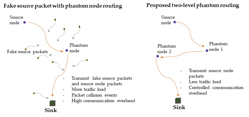
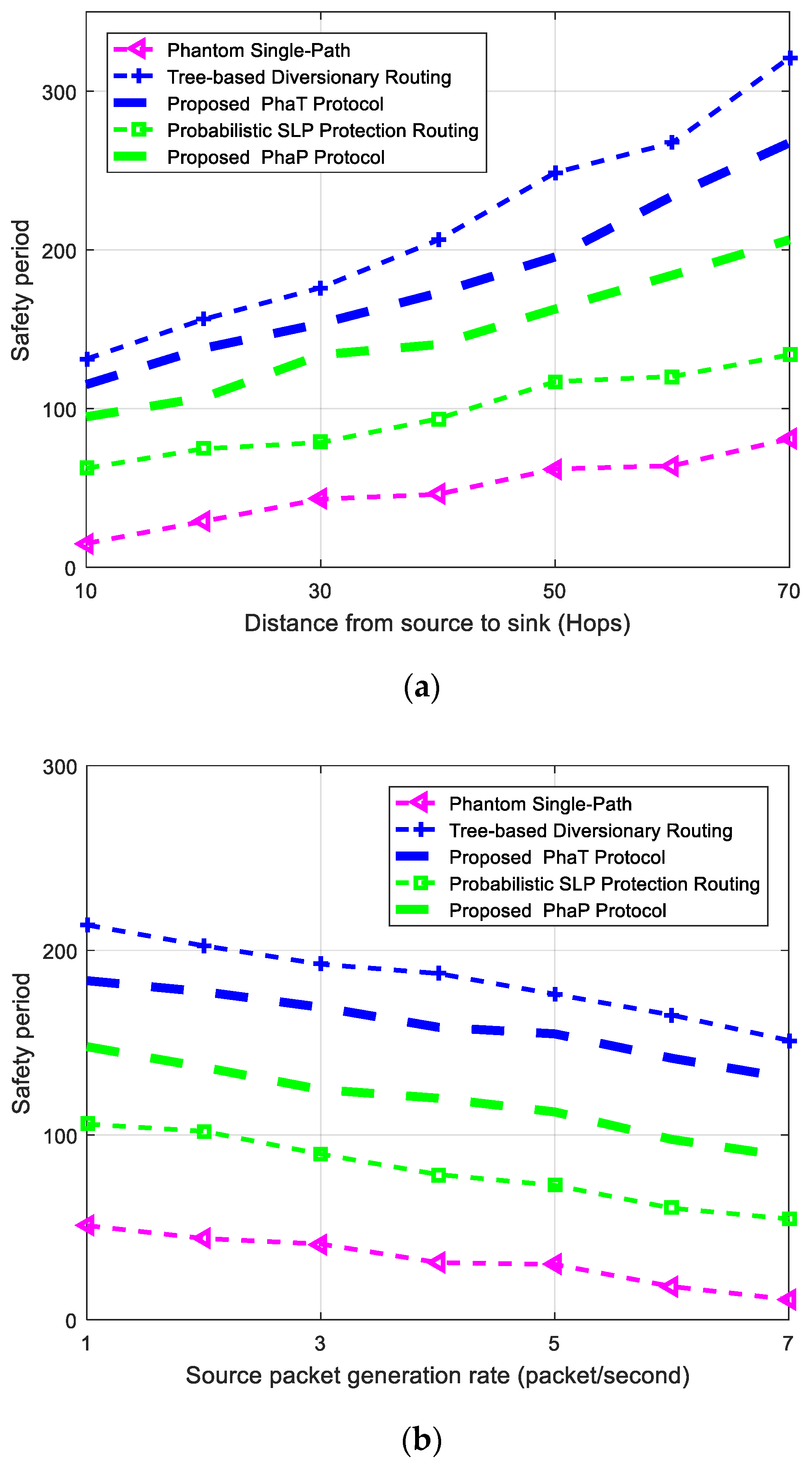
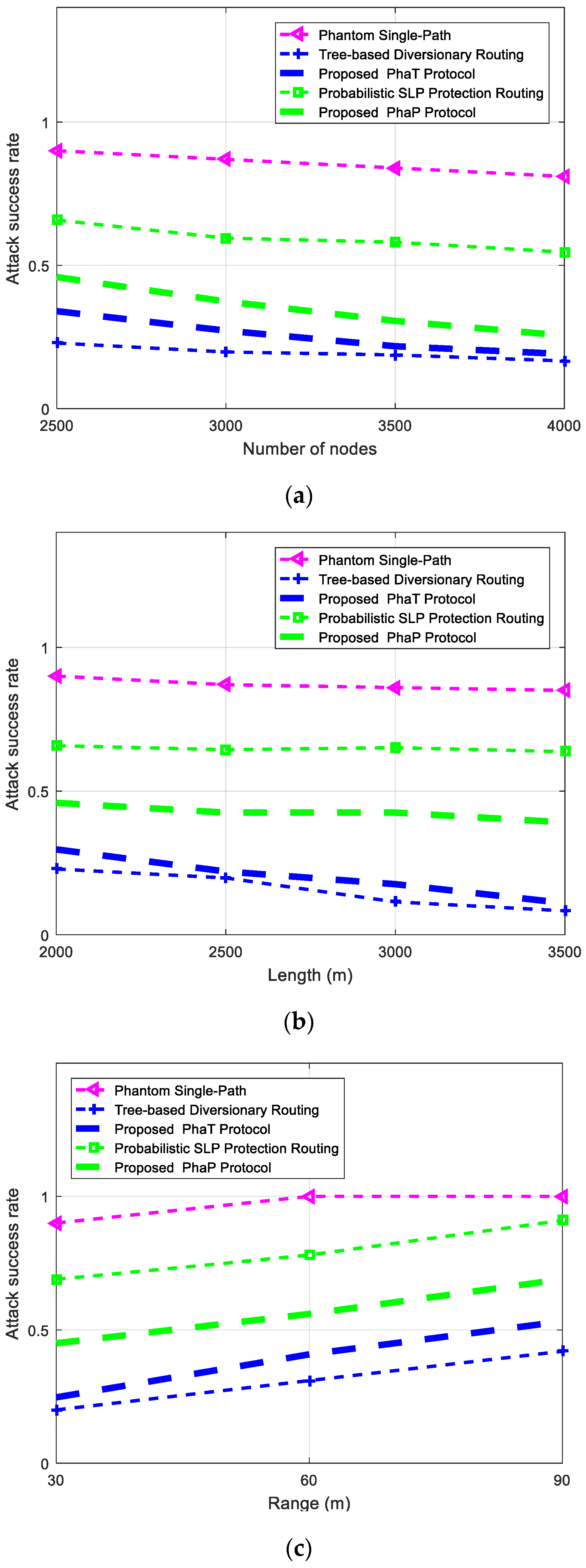
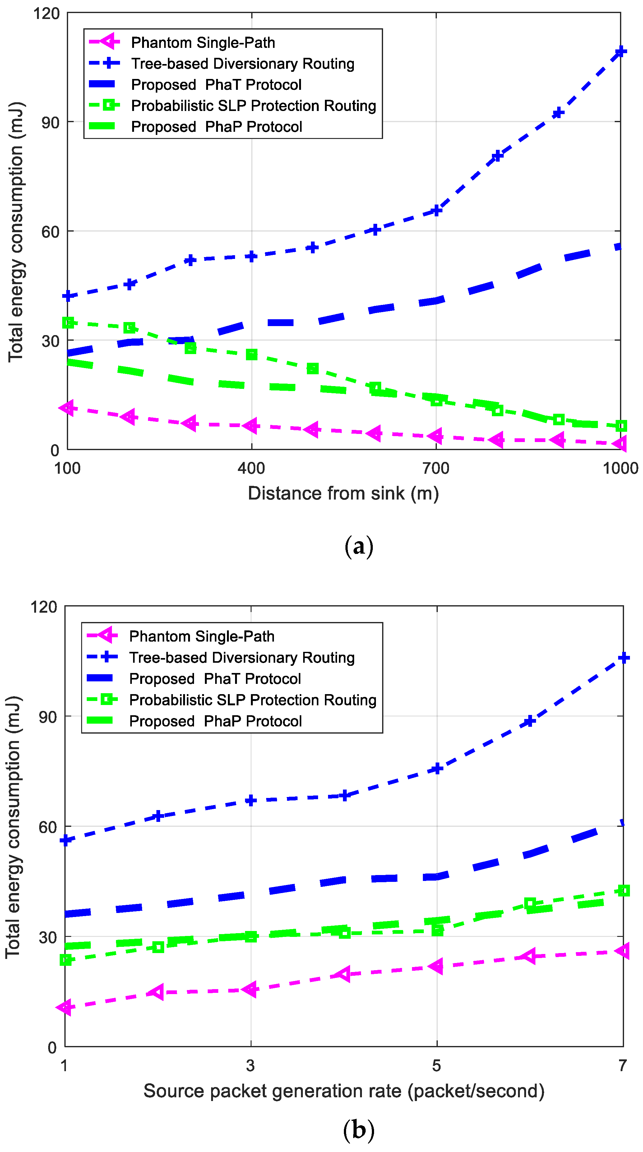
Table 1.
Summary of the performance features of the existing and proposed routing protocols.
| Protocol | Routing Strategy | Features | Influence |
|---|---|---|---|
| Tree-based diversionary routing (TreeR) [4]. | Integrates phantom routing and fake source packet routing. |
|
|
|
| ||
|
| ||
| Probabilistic source location privacy protection protocol (ProbR) [20]. | Integrates phantom routing and fake source packet routing. |
|
|
|
| ||
|
| ||
| Proposed two-level phantom with a backbone route (PhaT). | Replaces the fake source packets in TreeR with a second level phantom node. |
|
|
| Proposed two-level phantom with a pursue ring (PhaP). | Replaces the fake source packets in ProbR with a second level phantom node. |
|
|
Table 2.
Key differences between the routing strategies of the proposed and existing protocols.
| PhaP | ProbR |
|
|
|
|
| PhaT | TreeR |
|
|
|
|
Table 3.
Notations used in the proposed two-level phantom with a pursue ring (PhaP) protocol.
| Notation | Meaning |
|---|---|
| Pring | Pursue ring |
| dPin | Distance from the sink node to the inner ring of the Pring |
| dPout | Distance from the sink node to the outer ring of the Pring |
| PNfst | First level phantom node |
| PNsec | New second level phantom node |
| θ | Inclination angle between the X-axis and a line connecting the sink node and a node |
| TP | A bias threshold value |
| RN | A random number distributed between [0, 1] |
Table 4.
Selection of a second level phantom node (PNsec) according to the first level phantom node (PNfst) location and value of the random number (RN).
Table 4.
Selection of a second level phantom node (PNsec) according to the first level phantom node (PNfst) location and value of the random number (RN).
| Location of PNfst | Selection of PNsec | |
|---|---|---|
| RN < TP | RN ≥ TP | |
| East of the sink node (X-coordinate < 0) | PrNW | PrSE |
| West of the sink node (X-coordinate ≥ 0) | PrNE | PrSW |
Table 5.
Notations used in the proposed two-level phantom with a backbone route (PhaT) protocol.
| Notation | Meaning |
|---|---|
| epN | Existing first level phantom node adopted from TreeR |
| npN | New second level phantom node |
| dNB | Distance between the inner and outer boundaries of the near network border region |
| dSB | Distance from a sensor node to the network border |
| NNB | Nodes which are located in the near network border regions |
| RR | Restricted region around epN |
| dP | Hop distance between epN and npN |
| T | A bias threshold value |
| BN | Initial node of the backbone route, neighbor of npN |
| SF | A random selection factor distributed between [0, 1] |
Table 6.
Network simulation parameters.
| Parameter | Value |
|---|---|
| Network size (m2) | 2000 × 2000 |
| Number of nodes | 2500 |
| Number of sink nodes | 1 |
| dPin (m) | 400 |
| dPout (m) | 600 |
| TP | 0.5 |
| dH (hops) | 3 |
| dP (hops) | 4 |
| dNB (m) | 200 |
| T | 0.5 |
| Sensor node sensing range (m) | 30 |
| Adversary detection range (m) | 30 |
| Adversary waiting timer (source packets) | 4 |
| Adversary initial location | In the vicinity of the sink node |
| Source packet rate (packet/second) | Varied between 1 and 7 |
| Target monitoring scheme | k-nearest neighbors tracking |
Table 7.
Energy consumption model parameters.
| Parameter | Description | Value |
|---|---|---|
| Initial energy (J) | Initial energy of a sensor node | 0.5 |
| Eloss (nJ/bit) | Transmitting circuit energy loss | 50 |
| Eamp (pJ/bit/m4) | Energy for power amplification in the free-space model | 0.0013 |
| Efs (pJ/bit/m2) | Energy for power amplification in the multi-path attenuation model | 10 |
| do (m) | Threshold distance for the channel models | 87 |
| l (bit) | Size of the transmitted packet | 1024 |
© 2020 by the authors. Licensee MDPI, Basel, Switzerland. This article is an open access article distributed under the terms and conditions of the Creative Commons Attribution (CC BY) license (http://creativecommons.org/licenses/by/4.0/).
Share and Cite
MDPI and ACS Style
Mutalemwa, L.C.; Shin, S. Secure Routing Protocols for Source Node Privacy Protection in Multi-Hop Communication Wireless Networks. Energies 2020, 13, 292. https://doi.org/10.3390/en13020292
AMA Style
Mutalemwa LC, Shin S. Secure Routing Protocols for Source Node Privacy Protection in Multi-Hop Communication Wireless Networks. Energies. 2020; 13(2):292. https://doi.org/10.3390/en13020292
Chicago/Turabian StyleMutalemwa, Lilian C., and Seokjoo Shin. 2020. "Secure Routing Protocols for Source Node Privacy Protection in Multi-Hop Communication Wireless Networks" Energies 13, no. 2: 292. https://doi.org/10.3390/en13020292
Note that from the first issue of 2016, this journal uses article numbers instead of page numbers. See further details here.