An Iterative Scheme for the Power-Flow Analysis of Distribution Networks based on Decoupled Circuit Equivalents in the Phasor Domain

Abstract

This paper presents an alternative solution for the power-flow analysis of power systems with distributed generation provided by heterogeneous sources. The proposed simulation approach relies on a suitable interpretation of the power network in terms of a nonlinear circuit in the phasor domain. The above circuit interpretation can be solved directly in the frequency-domain via the combination of a standard tool for circuit analysis with an iterative numerical scheme, providing directly the steady-state solution of the power-flow of a generic distribution network. At each iteration, the resulting circuit turns out to be composed by two decoupled subnetworks, a large linear part and a set of smaller nonlinear pieces accounting for the load characteristics, with evident benefits in terms of the computational time. The feasibility and strength of the proposed simulation scheme have been verified on a large benchmark consisting of the IEEE 8500-node test feeder. Then it is applied to the statistical simulation of a power network accounting for the variability effects of renewable generators. According to the results, the proposed tool provides an effective alternative to the state-of-the-art approaches for power-flow analysis further highlighting the benefits of the application of well-established tools for circuit analysis to power-flow problems.

1. Introduction

From a very early time, the electrical power industry has faced many issues including generation-demand gap, reliability, planning, and operational back-offs and blackouts caused by weather and other external factors. In this framework, specific attention has been paid to the availability of modeling and simulation methods for both the transient and the steady-state assessment of the network state, also including a possibly large number of different heterogeneous distributed generator sources (DGs), nowadays spread into the power distribution networks. For the latter, several different analyses have been proposed in the literature including, power-flow, three phase-power flow, and harmonic analyses which have been proven to be mature tools successfully adopted in recent application problems [1,2,3,4]. Specifically, a probabilistic load flow with distributed wind generators is discussed in [1], a hybrid load flow involving multiple energy carriers is presented in [2], and the stochastic effects of the behavior of electric vehicles on the distribution networks is considered in [3].

Without loss of generality, efficient and reliable power-flow solution techniques have been developed and widely used for the assessment of power system operation [5,6,7,8]. Low resistive/reactive ratio for transmission lines (i.e., the so-called R/X factor) results in the decoupled real and reactive powers and thus few assumptions can be made to linearize the power-flow solution in terms of simple DC power-flow rather than AC power-flow [9,10,11,12]. However, it has repeatedly been shown that some conventional methods may become inefficient in the analysis of distribution networks. This becomes even more evident when the distributed generation units are integrated with a radial/meshed connected distribution system, and this integration is being increased day-by-day in form of renewable energy sources (wind, photo-voltaic, etc). Most of the methods available in the literature mainly focus on the power-flow analysis based on Newton–Raphson, Gauss–Seidel or backward/forward sweep algorithms for radial distribution networks [13,14,15,16,17,18,19]. Zhang in [13] modified the Newton–Raphson algorithm in which the Jacobian matrix is formed by backward/forward sweep, Teng [14] proposed a method based on mixing the so-called Z bus and traditional Guass–Siedal method to solve three-phase equations separately and obtains a closed-form solution, [15] implements backward/forward sweep for three-phase power flow and extend the method to find optimal feeding points for the reactive power compensation. For radial feeders only, Teng in [16] proposed a solution by forming a relation between bus injections and bus voltages directly through matrices based on backward/forward sweep algorithm. Eminoglu and Hocaoglu in [17] used polynomial equations to solve nodal voltages and backward propagation for branch currents. The above method, however, turns out to be slower compared to other sweep algorithms. In [18], algebraic recursive equations are used for power flow solution, and Garces in [19] proposed linear approximation on the complex plane to solve unbalanced power flow equations without taking into account the PV nodes for loads/DGs. It important to point out that the solution of weakly meshed networks requires in general custom adjustments in which the network is first converted into an equivalent radial network by breaking the looping branches, with detrimental impacts on accuracy, efficiency and simplicity of the solution. Recently, Bazrafshan et al. [20] proposed a new approach for the modeling of a three-phase distribution system based on the Z Bus method, which however does not explicitly exploit the radial and weakly meshed network structure of distribution systems and it requires the solution of a set of equations whose size is proportional to the number of buses (and/or looping branches). As a result, it converges for weakly meshed configuration only under some specific assumptions, as pointed out in [21]. A different formulation of the power-flow analysis for both power transmission and distribution networks by means of a circuital interpretation of the network and the application of classical tools for circuit analysis are instead presented in [22,23,24], offering a general solution with improved convergence for very large structures including weakly and heavily meshed structures.

This paper focuses on the latter class of approaches and discusses a different interpretation of the power distribution network in terms of a nonlinear circuit in the f-domain. The resulting circuit is then analyzed by combining the modified nodal analysis (MNA) [25] with an iterative scheme based on the waveform relaxation technique [26]. It allows decoupling the solution of the inherent nonlinear problem in the harmonic domain into the solution of a large linear network followed by a subsequent nonlinear computation related to some of the network components only (e.g., renewable sources). The approach is simple and general, and applies to any kind of network, including meshed structures. It is important to point out that the proposed contribution shares the idea of using a circuit based approach which has already been proven to be general and robust in terms of convergence [23]. The proposed method is a viable alternative that can be readily applied to the number of alternative applications, including the co-simulation of multi-energy networks, possibly including gas distribution systems [27]. This is possible since it uses the same philosophy of dealing with steady-state operation and a compact matrix formalism which is directly linked to the graph description of the network. An additional important feature of this approach relies on its flexibility allowing the application of alternative numerical schemes (such as Netwton–Rapson or fixed-point iteration, being the latter considered in this paper only) without changing the proposed circuital interpretation. It is also verified that at each iteration of the method, the resulting circuit can be alternatively solved by any simulation program with integrated circuit emphasis (SPICE) solver at a single frequency AC analysis.

This paper is organized as follows. Section 2 describes the proposed numerical simulation of distribution networks, including additional details on the definition of loads. Section 3 collects the validation of the method and its application to standard test cases. The three-phase IEEE 8500-node test feeder is considered as the initial state-of-the art benchmark example. A second validation involving a smaller test case with renewable generators is then included and solved by both our custom MATLAB implementation of the equations and SPICE. For the latter example, the statistical analysis of the distribution network aimed at assessing the inclusion of the variability effects of distributed generators concludes the application results. Final remarks and conclusions are given in Section 4.

Table 1. List of acronyms.

DGs	Distributed generator sources
MNA	Modified nodal analysis
SPICE	Simulation program with integrated circuit emphasis
PQ	Generator node with real and reactive power
PV	Generator node with real power and voltage magnitude
PQ(V)	Generator node with real power and voltage dependent reactive power
EPRI	Electric Power Research Institute
MV	Medium voltage
LV	Low voltage
OpenDSS	Open source distribution system simulator

lists all the acronyms used in the text.

2. Power-Flow Analysis and Numerical Simulation

This section presents the simulation technique proposed in this paper for the power-flow analysis of a generic distribution network with renewables. The proposed solution relies on a circuit interpretation of the network along with its distributed generators in terms of a nonlinear circuit in the phasor domain, which is then solved via the standard tools for the circuit analysis.

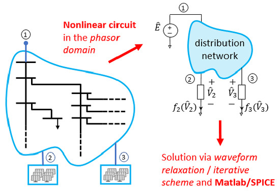
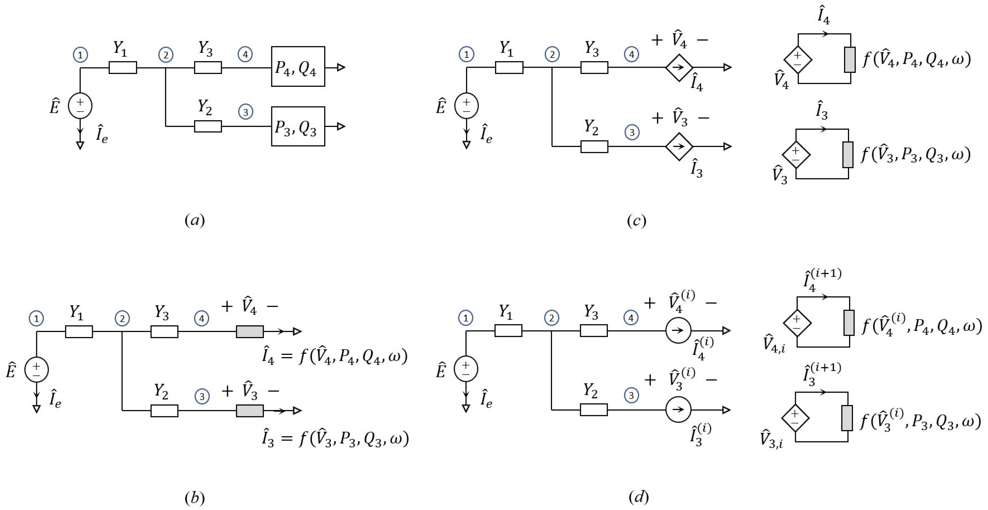
2.1. Circuital Equivalent of a Distributed Network in the Phasor Domain

For the sake of illustration, the following discussion focuses on the example network shown in Figure 1a. It consists of a simple radial power distribution network fed by an ideal sinusoidal voltage source with phasor $\widehat{E}(\omega )$, in which the transmission lines are described by lumped $RL$ equivalents represented by the gray blocks, whereas the circuital elements connected to the nodes 3 and 4 correspond to either an absorbing load or a renewable source providing a complex power $S_3=P_3+j{Q}_3$ and $S_4=P_4+j{Q}_4$, respectively. Further details on possible alternative characterization of the network loads are provided at the end of this section.

The above distribution network can be interpreted via the equivalent circuit in the phasor domain depicted in Figure 1b. It consists of a nonlinear circuit in frequency-domain which provides a nonlinear map in the complex domain between a given set of isofrequential excitations at frequency $\omega$ and the corresponding phasors of the voltage and current responses at each node of the network.

To this aim, the loads of the network connected at node 3 and 4, characterized in terms of their adsorbed or produced power, have been readily converted into the corresponding nonlinear voltage controlled current sources $f({\widehat{V}}_k)$ defined through the complex power $S_k={\widehat{V}}_k{\widehat{I}}_k^{*}$, yielding:

$${\widehat{I}}_k=f({\widehat{V}}_k;P_k,Q_k,\omega )={\left(\frac{P_k+j{Q}_k}{{\widehat{V}}_k}\right)}^{*},$$

(1)

where $P_k$ and $Q_k$ are the active and reactive power for a load at node k (e.g., $k=3$ and 4).

It is important to remark that the circuit schematic in Figure 1b can be easily described via the MNA [23,25], which represents one of the most established formulations for the solution of linear and nonlinear circuits, since it is currently used in a number of commercial simulation software such as SPICE. Specifically, according to the procedure in [25] the MNA allows analyzing the circuit in Figure 1b from topological inspection only, leading to the following matrix form:

$$\widehat{\mathbf{M}}\widehat{\mathbf{W}}={\widehat{\mathbf{A}}}_0+\widehat{\mathbf{A}}(\widehat{\mathbf{W}}),$$

(2)

where $\widehat{\mathbf{W}}\in {\mathbb{C}}^5$ is a complex vector collecting the nodal voltages and the currents flowing through current controlled elements, i.e., $\widehat{\mathbf{W}}={[{\widehat{V}}_1,{\widehat{V}}_2,{\widehat{V}}_3,{\widehat{V}}_4,{\widehat{I}}_e]}^T$, ${\widehat{\mathbf{A}}}_0\in {\mathbb{C}}^5$ is a complex vector collecting the independent sources of the circuit, i.e., ${\widehat{\mathbf{A}}}_0={[0,0,0,0,\widehat{E}]}^T$ and $\mathbf{M}$ is a complex matrix, readily derived from the topology of the circuit in Figure 1b by inspection, which writes:

$$\begin{array}{c}\hfill \widehat{\mathbf{M}}=\left[\begin{array}{ccccc}{Y}_1& -Y_1& 0& 0& 1\\ -Y_1& Y_1+Y_2+Y_3& -Y_2& -Y_3& 0\\ 0& -Y_2& Y_2& 0& 0\\ 0& -Y_3& 0& Y_3& 0\\ 1& 0& 0& 0& 0\end{array}\right].\end{array}$$

(3)

In the above equation $Y_i=1/(R_i+j\omega L_i)$ for $i=1,2$ and 3, where the dependency from the angular frequency $\omega$ is omitted for compactness. Furthermore, the complex vector $\widehat{\mathbf{A}}(\widehat{\mathbf{W}})$ accounts for the nonlinear I-V characteristic of the network load and renewable elements:

$$\begin{array}{c}\hfill \widehat{\mathbf{A}}(\widehat{\mathbf{W}})={\left[0,0,-f({\widehat{V}}_3;P_3,Q_3,\omega ),-f({\widehat{V}}_4;P_4,Q_4,\omega ),0\right]}^T.\end{array}$$

(4)

2.2. Fixed Point Iteration Via Circuital Interpretation

Unfortunately, a trivial closed-form solution of the transcendental equation given by the MNA in (2) is not available, therefore such an equation must be solved numerically. Without loss of generality, the numerical analysis proposed hereafter focuses on a fixed-point iteration scheme.

The discussion starts considering the nonlinear circuit in Figure 1c, in which the linear and nonlinear portions of the network have been split into two sub-networks coupled through current and voltage controlled sources, respectively. It is important to remark that the above circuit turns out to be equivalent to our original network in Figure 1b. However, the proposed interpretation is the first step toward the so-called relaxation of the nonlinear problem.

The new interpretation of the nonlinear circuit in the phasor domain can be relaxed by replacing the voltage controlled current source in the linear network with an independent current sources of value ${\widehat{I}}_3^{(i)}$ and ${\widehat{I}}_4^{(i)}$, as shown in Figure 1d. This means that we are decoupling the linear network form the nonlinear one. According to this, the nonlinear MNA equation in (2) can be approximated by the following iteration scheme [26]:

$$\begin{array}{c}\hfill \left\{\begin{array}{c}\widehat{\mathbf{M}}{\widehat{\mathbf{W}}}^{(i)}={\widehat{\mathbf{A}}}_0+{\widehat{\mathbf{A}}}^{(i)}\hfill \\ {\widehat{\mathbf{A}}}^{(i+1)}=\widehat{\mathbf{A}}({\widehat{\mathbf{W}}}^{(i)}),\hfill \end{array}\right.\end{array}$$

(5)

where ${\widehat{\mathbf{A}}}^{(i)}={[0,0,-{\widehat{I}}_3^{(i)},-{\widehat{I}}_4^{(i)},0]}^T$ is a vector collecting the amplitude at the i-th iteration of the independent current sources connected to the linear portion of the proposed network interpretation (see the left part of the schematic in Figure 1d) and ${\widehat{\mathbf{A}}}^{(i+1)}$ is a vector collecting the phasors of the currents flowing through the voltage controlled sources in the non-linear portion of the circuit (see the right part of the schematic in Figure 1d) defined by the voltages in ${\widehat{\mathbf{W}}}^{(i)}$ and (4) as follows:

$$\begin{array}{c}\hfill {\widehat{\mathbf{A}}}^{(i+1)}=[0,0,f({\widehat{V}}_3^{(i)};P_3,Q_3,\omega ),f({\widehat{V}}_4^{(i)};P_4,Q_4,\omega ),0].\end{array}$$

(6)

Iterating the above equation leads to the following update rule:

$$\begin{array}{c}\hfill {\widehat{\mathbf{W}}}^{(i+1)}={\widehat{\mathbf{M}}}^{-1}({\widehat{\mathbf{A}}}_0+\widehat{\mathbf{A}}({\widehat{\mathbf{W}}}^{(i)})).\end{array}$$

(7)

The above equation is iterated until a given convergence criterion is reached. A widely used idea is to use the $L_{\infty }$-norm error between the value of the unknown vector $\widehat{\mathbf{W}}$ at current i-th iteration and the new prediction $(i+1)$-th is less than a given threshold $\epsilon$:

$$\parallel {\widehat{\mathbf{W}}}^{(i+1)}-{\widehat{\mathbf{W}}}^{(i)}{\parallel }_{L_{\infty }}\le \epsilon .$$

(8)

The iterative rule in (7) derived from the relaxed circuit interpretation of the nonlinear MNA equation, turns out to be an alternative interpretation of the fixed-point iteration in the complex domain (see Appendix A for additional details).

The main advantages of the proposed formulation is that the linear portion of the system, which is usually large, needs to be solved only once during the iteration (i.e., the inverse matrix ${\widehat{\mathbf{M}}}^{-1}$ must be computed once since all the entries are known and do not vary). Also, different from the Newton–Rapshon iterative scheme usually used for the analysis of non-linear circuits in time-domain, the proposed technique does not require to compute the Jacobian matrix of the system, thus simplifying its implementation. The above simplification is motivated by the fact that, since we are working in the frequency-domain, the MNA equation turns out to be a static nonlinear equation in the complex domain (i.e., the equation does not contain any differential operator), thus leading to a simpler solution compared to more common dynamical cases. However, if it is needed, the iteration rules of the proposed approach based on the fixed-point scheme can be easily rearranged in order to cope with the more computationally expensive Netwon–Raphson method, being the latter a different interpretation of the proposed fixed-point technique. Moreover, the adopted circuital interpretation of a distribution network readily allows the circuit implementation in any SPICE solver (e.g., HSPICE, PSPICE, LTspice) with the solution in AC at a single frequency point. Additional details on the above feature will be provided in Section 3.2.

2.3. Source and Load Definition

Distributed generation sources (DGs) of the network can be described by small generators connected at various nodes in the distribution system to reduce the generation demand gap and improving both the reliability and voltage profiles across the network. They are connected in different configurations like power factor-controlled, voltage-controlled, or current-controlled modes. DGs can be traditional generators or renewable energy devices (photovoltaic, wind, fuel cells, etc.). (e.g., the blocks $P_3$, $Q_3$ and $P_4$, $Q_4$ in the schematic of Figure 1a). At any node, there are four parameters, real power (P), reactive power (Q), voltage magnitude (V) and voltage angle ($\theta$). During the analysis, any two variables are known and two unknowns, thus DGs are classified into the type of known variables as PQ, PQ(V), PV (or PI). Since this work focuses only on renewables, the DGs term used hereafter refers to renewable energy sources, only.

Based on the information provided for the definition of the various types of DGs, each generator can be readily converted into a current source as briefly done for the simple PQ case in Section 2. For the PQ(V) case, current injection is still done via (1) because DG’s real power and reactive power are specified, with the exception that the reactive power turns out to be defined as a function of the voltage magnitude. For the PV type, instead, the specified values of DG are the real power output and bus voltage magnitude. To calculate the equivalent current injections for this type, an iterative process is required. The mentioned procedure, further explained in [28,29], calculates the reactive power of the DG necessary to keep the bus voltage magnitude on the specified value. After the required power has been obtained, the equivalent current injection is computed as in (1) and integrated into (7) to calculate power-flow results.

3. Numerical Results

In this section, the effectiveness of the proposed approach for the power-flow analysis is investigated by considering two test cases. The first one consists of the benchmark IEEE 8500-node test feeder which represents a realistic full-size distribution system [30,31]. This first distribution network is aimed at validating the method and discussing its performance in terms of accuracy, efficiency, and convergence. Then, a second test case consisting of a single-phase network with 90 nodes is solved via the proposed approach for the power-flow analysis by considering both the MATLAB and its implementation in a commercial SPICE-based solver (i.e., LTspice from analog devices is used in this comparison). The obtained results are then validated via OpenDSS. The same network is then used for a practical application in which the DGs are spread along the network. For this second example, a statistical simulation for the systematic assessment of the possible effects of the variability of power rating of the DGs is carried out. For all the validations and applications, the tolerance $\epsilon$ in (8) is set to ${10}^{-4}$.

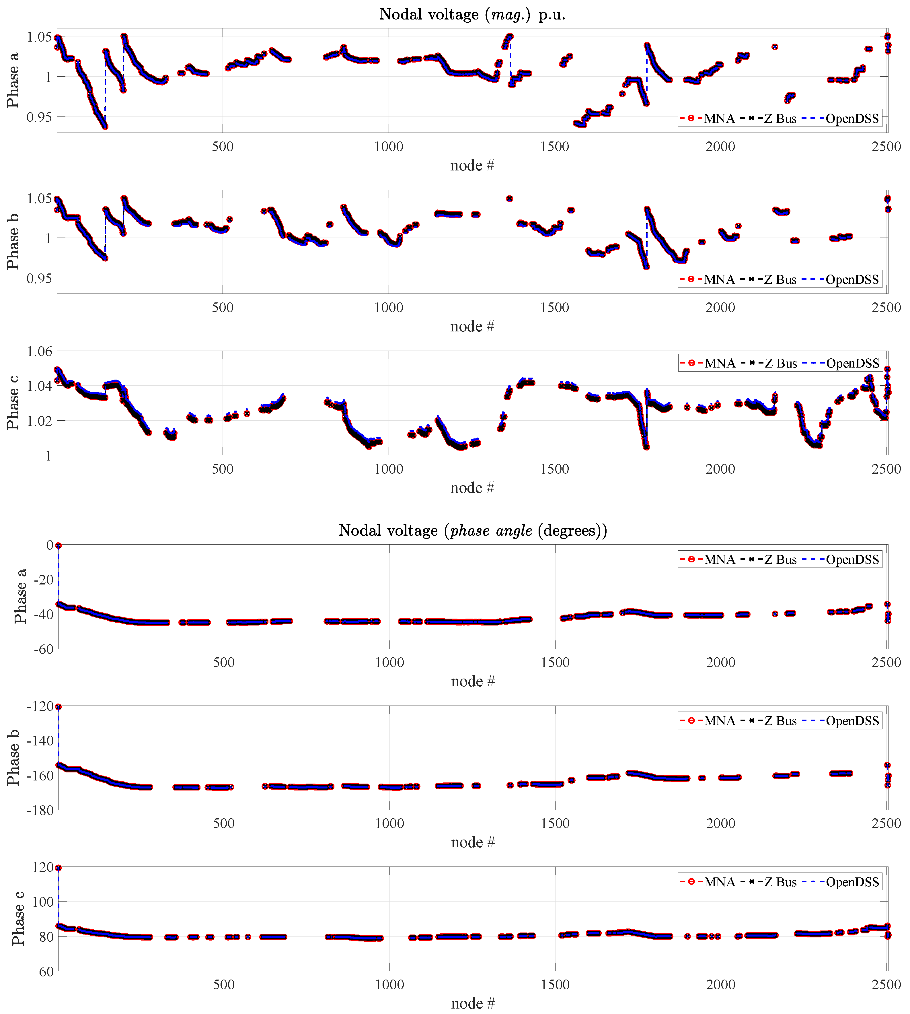
3.1. Validation: IEEE 8500-Node Test Feeder

The IEEE 8500 benchmark is considered for the performance assessment of the proposed simulation scheme. It is a large three-phase unbalanced radial network having both MV (medium voltage, primary distribution) and LV (low voltage, secondary distribution) levels and includes most of the components available in a typical North American medium voltage distribution feeder. The placement of the regulators and capacitors on the test feeder are shown in Figure 2. The three-phase network is analyzed through the proposed method detailed in Section 2, yielding to an unavoidable increase in the size of the involved matrices. Both the magnitude and the angle of the nodal voltages associated with the three lines, hereafter labeled as phases a,b and c, are computed. It is important to point out that transformers and regulators are modeled as in [20,32]. In addition, fixed regulator taps are considered as published in [24]. In order to provide a fair validation, the obtained results are compared with the ones obtained by means of the Z Bus method [20,33] and of the open source distribution system simulator (OpenDSS) [34], being the latter a reference tool released by the Electric Power Research Institute (EPRI).

The voltage magnitudes and angles computed by the three methods are shown in Figure 3, highlighting identical results. In addition,

Table 2. Performance of the different methods in terms of convergence for the IEEE 8500-node benchmark.

Method	Iterations	CPU Time (ms)
Proposed (MNA)	11	96.6
Z Bus	12	101.1
OpenDSS	10	53.4

proposes a compact summary of the performance of the differed methods in terms of simulation time and number of iterations. The above numbers are generated running the scripts on a PC equipped with a CPU Intel Core i7 (seventh generation) and 32 GB ram. In addition, for the proposed approach, Figure 4 shows the maximum voltage difference computed at each iteration, highlighting the typical decreasing staircase behavior of fixed-point convergence where the horizontal line shows the convergence tolerance set to ${10}^{-4}$. The above figures and table highlight that the proposed approach has been proven to provide accurate results without any simulation overhead in terms of simulation time. It offers the unavoidable benefit of being general and flexible, thus not requiring any custom solutions for any arbitrary network.

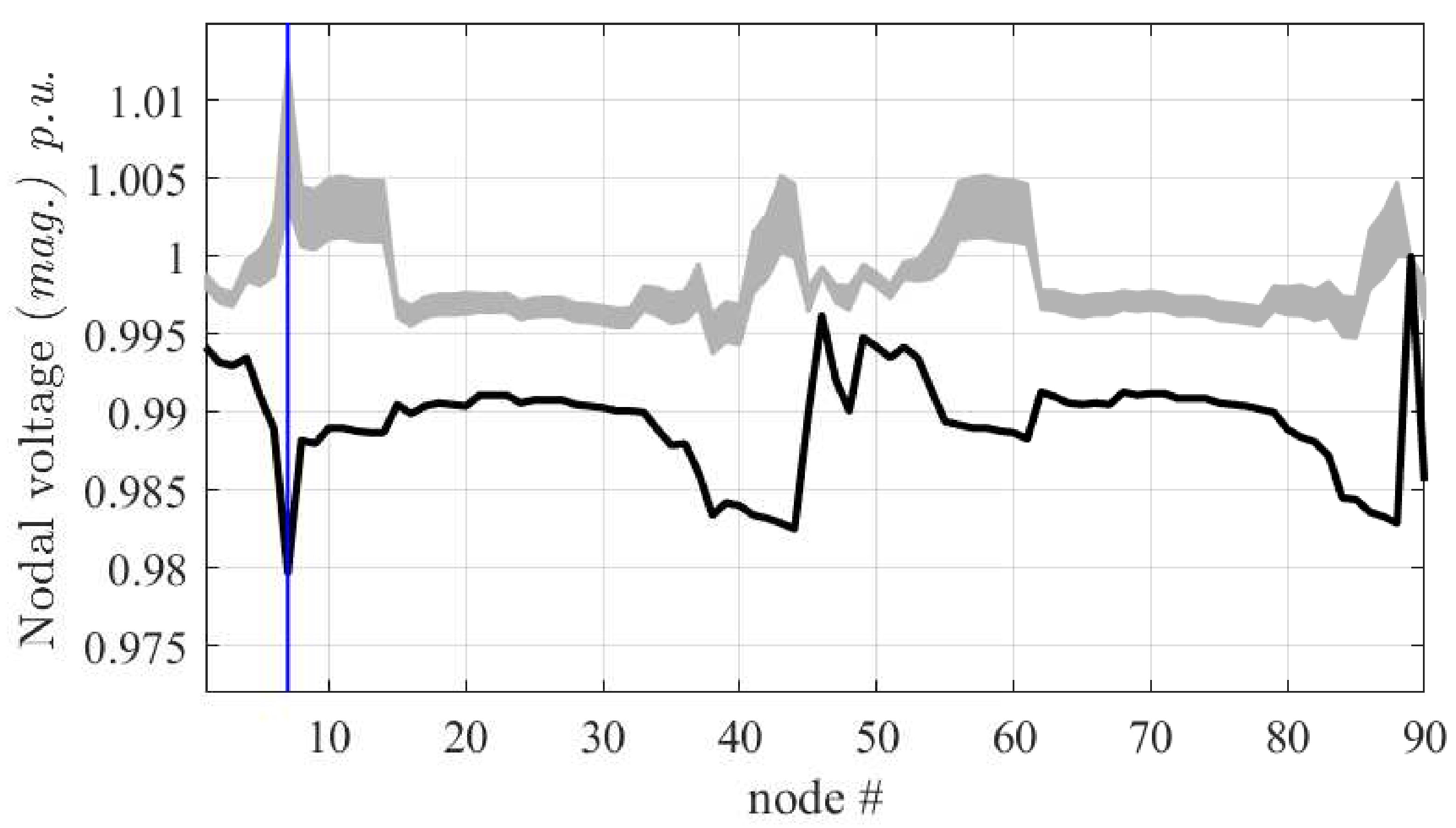
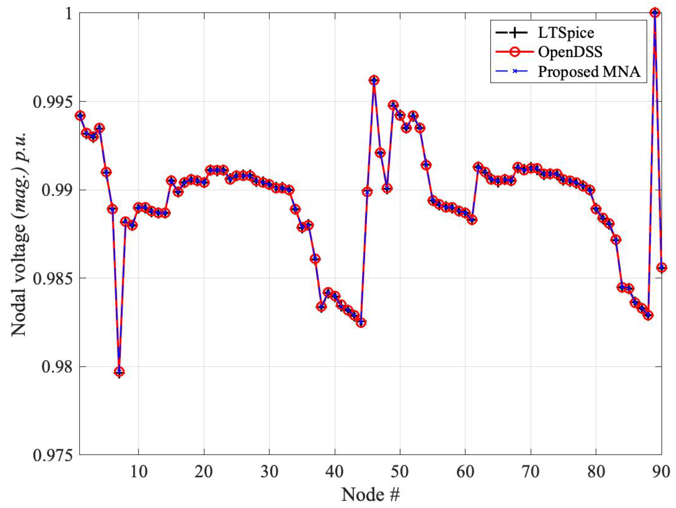
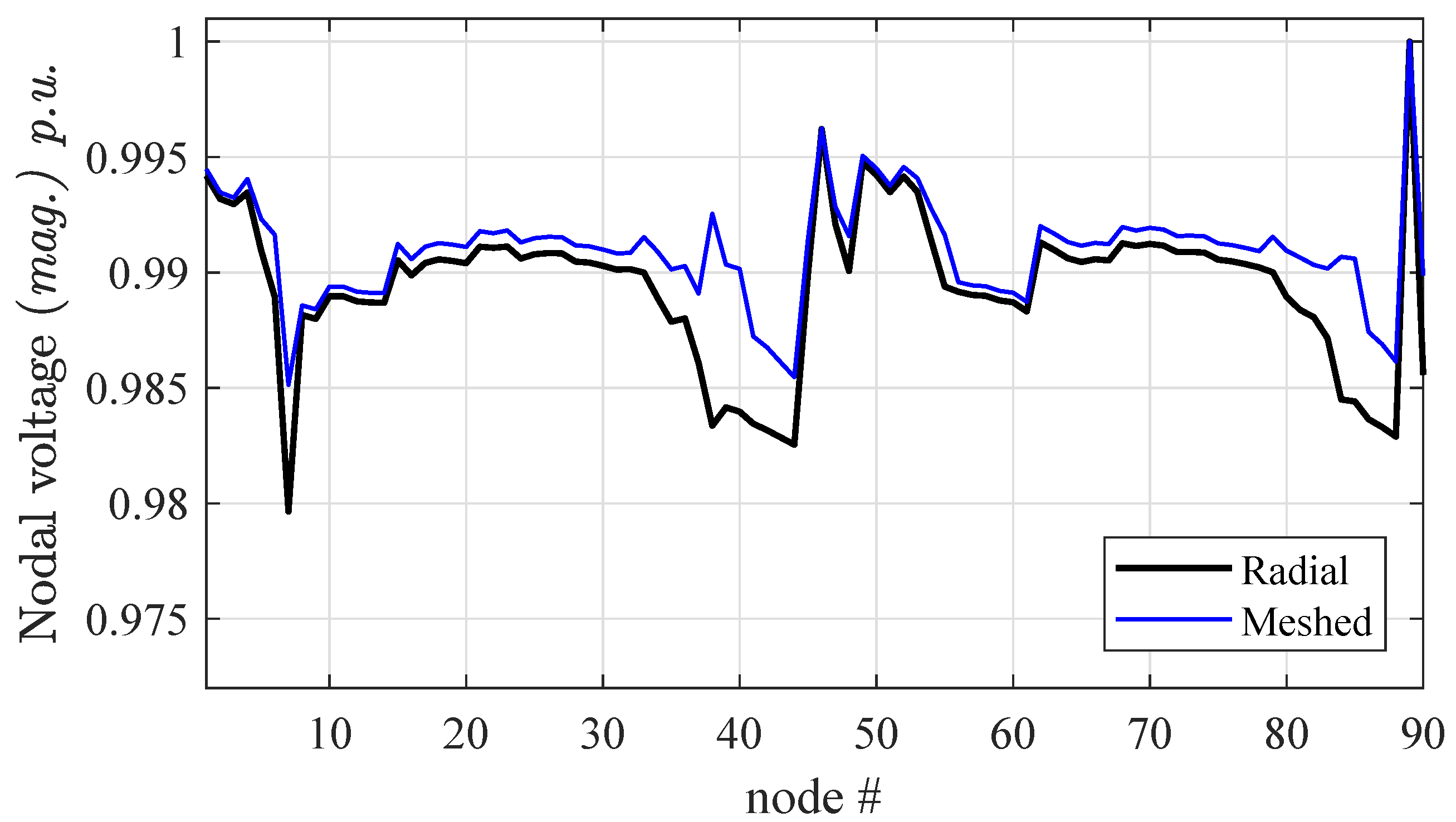
3.2. Validation: 90-Node Single Phase Network

The test case considered in this section is a $10$ kV single-phase radial distribution system with no transformers and regulators, hereafter termed as Test90. The topological structure of this test network is shown in Figure 5 and the parameters and data can be found in [35]. The network has been implemented within the simulation framework described in Section 2. For the validation, no DGs are connected and all the loads are PQ type and their corresponding current injections are calculated using Equation (1).

Figure 6 shows the voltage magnitude curve solved through the propsosed MNA method validated with OpenDSS program. The same network is also solved through LTspice by replacing the MNA solution with a SPICE-based solution, leading to overlapped responses. The above comparison also stresses the flexibility of the proposed approach in allowing either a custom MATLAB implementation of the equations or the direct use of any classical software for circuit analysis. The circuital simulation is carried out in AC at the single operating frequency. The netlist is automatically generated based on the topology of the network and on the load definitions at each step of the iterative procedure and is feeding the LTspice solver which produces the phasor responses of the nodal voltages.

As an additional analysis, the considered Test90 power distribution is suitably modified as a weakly meshed network by closing the connections between the three dashed lines that represent tie branches (see Figure 5). The results of this test are shown in Figure 7. It is worth noting that the convergence for radial and weakly meshed networks are on the same order of magnitude of the first example, leading in this case to few dozens of milliseconds of CPU time (e.g., $16.9$ ms for the radial configuration and $18.2$ ms for the weakly meshed one). What is more important, the branches with a loop are treated in the same way, stressing again the generality of the proposed approach.

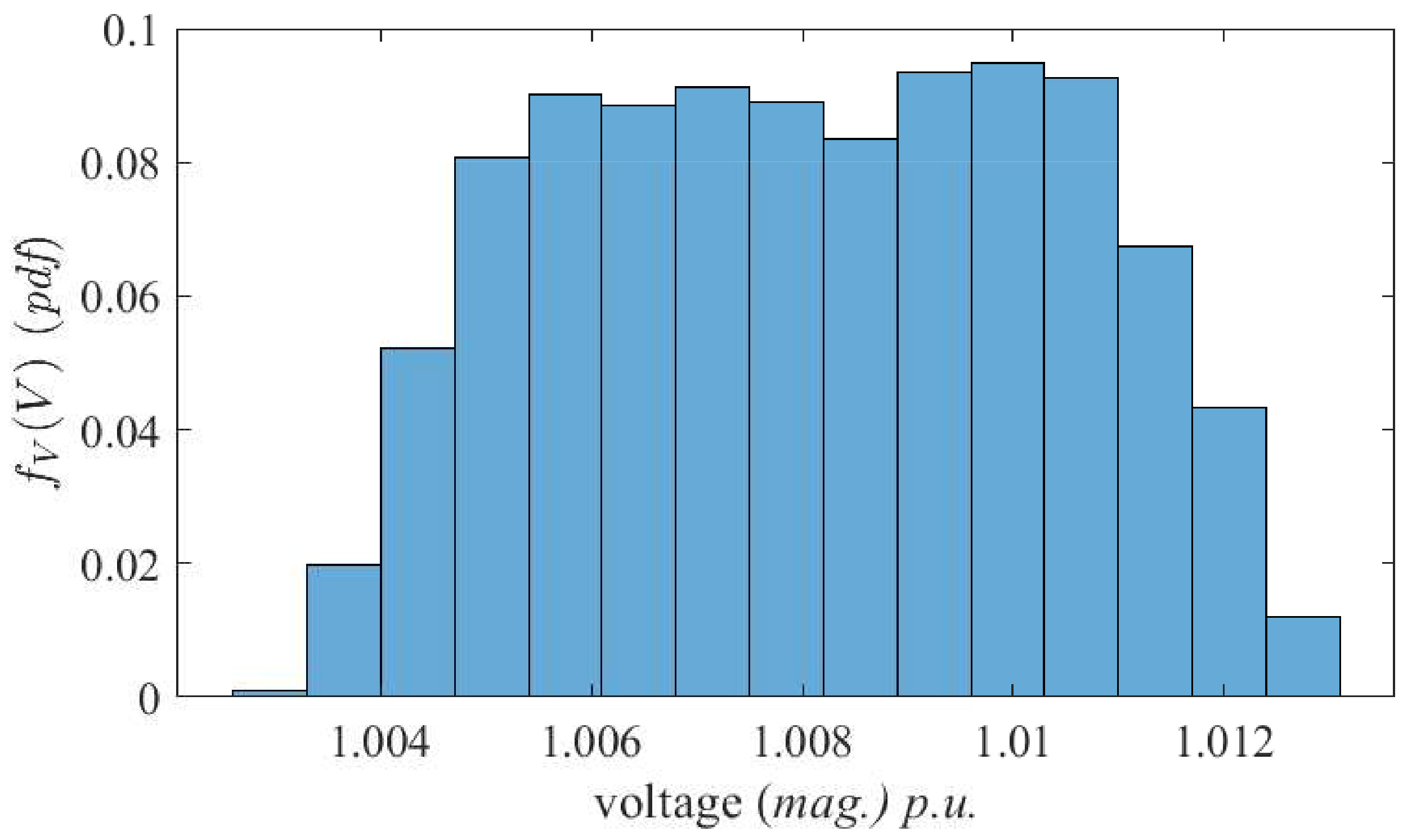
3.3. Application: DGs and Stochastic Analysis

In this section, a practical application is carried out for Test90 network where DGs are spread along the network. A statistical simulation aimed at assessing the effects of DGs (either in terms of location but specifically in terms of power generation).

Table 3. Description for different cases of Test90.

Case	DG Node(s)	Type	P (p.u.)	Q (p.u.)	V (p.u.)
Case I	No DGs	-	-	-	-
	7	PQ	0.3	0.3	-
	20	PQ	0.1	0.1	-
	37	PQ	0.234	0.234	-
	43	PQ	0.1	0.1	-
	44	PQ	0.05	0.05	-
	58	PQ	0.19	0.19	-
Case II	61	PQ	0.03	0.03	-
	63	PQ	0.18	0.18	-
	68	PQ	0.12	0.12	-
	81	PQ	0.05	0.05	-
	84	PQ	0.08	0.08	-
	88	PQ	0.3	0.3	-
	7	PV	0.3	-	1.00
	20	PQ	0.1	0.1	-
	37	PQ	0.234	0.234	-
	43	PV	0.1	-	1.00
	44	PQ	0.05	0.05	-
	58	PQ	0.19	0.19	-
Case III	61	PQ	0.03	0.03	-
	63	PQ	0.18	0.18	-
	68	PQ	0.12	0.12	-
	81	PQ	0.05	0.05	-
	84	PQ	0.08	0.08	-
	88	PV	0.3	-	1.00

provides additional details on the different configurations considered for this alternative application in which DGs are not included in the system (case I) or placed in different locations (cases II and III). The latter two cases include PQ and PV types of DGs, for which reactive power is corrected at each iteration according to [28,29] as stated in Section 2.3.

Figure 8 collects the results of the simulation of the network for the above-mentioned configurations, thus highlighting the deterministic impact of the DGs, along with their placements. As a second and more realistic application, the Test90 radial distribution network is analyzed for variability analysis of DGs power ratings, to simulate practical conditions when DGs are spread along the network. Specifically, the power of DGs is assumed not being constant but is varying throughout the day according to weather conditions, with the aim of observing the change in the voltage profile. Two tests are carried out, based on Monte Carlo simulations performed by varying DGs power in the range $[-20,20\%]$ around their nominal rated capacity (see Figure 9), and in the range $[0,100\%]$ (see Figure 10). The latter case corresponds to an extreme simulation stressing the wide range of effects arising from the possible unpredictable behavior of DGs. In addition, Figure 11 shows the probability density function of the voltage of node 7 (i.e., the node with the highest load). From Figure 10 the band in the voltage profile is observed and the behavior of the distribution network (which relies largely on DGs) can be predicted. This can help utility and stakeholders to understand the effects of renewables’ variability and unhealthiness of the network. It is to state that Monte Carlo simulation is used to observe the stochastic behavior of the network because we keep only two or three parameters of DGs as varying so simple Monte Carlo method holds, however, if the number of parameters is large, other methods are preferable for analyzing the uncertain behavior [36,37,38,39].

4. Summary and Conclusions

This paper addressed the compact modeling of a power distribution system using an alternative approach relying on a circuital interpretation of the network in terms of a nonlinear circuit in the phasor domain. A standard MNA formulation for circuit analysis is adopted and the resulting matrix equation is solved via a fixed-point iterative scheme, offering a simple solution in which the original network is split into a large linear part combined with and a sparse nonlinear portion. The validation and applications performed, which focused on two test cases, the so called Test90 network and the widely adopted benchmark IEEE 8500-node test feeder, proved that the approach offers good performance in terms of both simulation time and accuracy and turns out to be an excellent alternative candidate to be effectively used for large networks with multiple dispersed generators. A final application involving the statistical simulation of the Test90 network accounting for the uncertain effects of renewable generators is carried out.

It is important to point out that the fixed-point numerical scheme is chosen for demonstrating that even for realistic large networks, this choice offers a viable and efficient solution that does not require the computation of auxiliary matrices (such as the Jacobian matrix) at each step of the simulation procedure. The proposed method is, however, independent form the numerical scheme adopted and if needed, for problematic cases, other iteration schemes such as Newton–Rapson can be effectively adopted. In addition, the interpretation of the original network as the circuit of Figured possibly allows replacing the MATLAB MNA formulation of the network with a more intuitive circuital formulation which can be suitably implemented within any commercial SPICE-like solver. The above feature, which introduces additional user’s flexibility and also allowed cross-validating the proposed technique, has been applied to the Test90 case. As a final summary, the key highlights and outcomes of this paper are:

• Verify the feasibility of using the waveform relaxation technique [26] to the power-flow analysis of power networks. This allows decoupling the inherent nonlinear network into the combination of a large linear subpart and a nonlinear portion, unavoidably enabling any tool for speeding up the simulation of the linear part;
• Demonstrate that the load flow analysis can be effectively carried out via standard tools for circuit analysis such as the MNA [25] (as done in other papers in literature as [23]), but also possibly replacing the simulation of the decoupled network via any SPICE-based commercial tool;
• Offer a flexible iterative procedure, which is combined with the simplest possible numerical scheme such as the fixed-point iteration. The mentioned procedure can be readily modified to incorporate other schemes such as Newton–Rapson;
• Verify that without working on the fine optimization of the routines, the implementation of the MNA-based formulae in MATLAB still produces the same accuracy and computational efficiency of reference commercial tools (e.g., OpenDSS) and of other custom implementations of state-of-the art load flow analyses (e.g., [20]).

References

1. Oshnoei, A.; Khezri, R.; Hagh, M.T.; Techato, K.; Muyeen, S.M.; Sadeghian, O. Direct Probabilistic Load Flow in Radial Distribution Systems Including Wind Farms: An Approach Based on Data Clustering. Energies 2018, 11, 310. [Google Scholar] [CrossRef] [Green Version]
2. Bockl, B.; Greiml, M.; Leitner, L.; Pichler, P.; Kriechbaum, L.; Kienberger, T. HyFlow—A Hybrid Load Flow-Modelling Framework to Evaluate the Effects of Energy Storage and Sector Coupling on the Electrical Load Flows. Energies 2019, 12, 956. [Google Scholar] [CrossRef] [Green Version]
3. Yang, J.; Hao, W.; Chen, L.; Chen, J.; Jin, J.; Wang, F. Risk Assessment of Distribution Networks Considering the Charging-Discharging Behaviors of Electric Vehicles. Energies 2016, 9, 560. [Google Scholar] [CrossRef] [Green Version]
4. Corrêa, H.P.; Vieira, F.H.T. Load Flow Independent Method for Estimating Neutral Voltage in Three-Phase Power Systems. Energies 2019, 12, 3216. [Google Scholar]
5. Stevenson, W.D. Elements of Power System Analysis, 4th ed.; McGraw-Hill: New-York, NY, USA, 1982. [Google Scholar]
6. Tinney, W.F.; Hart, C.E. Power flow solutions by Netwon’s method. IEEE Trans. Power Appar. Syst. 1967, 86, 1449–1460. [Google Scholar] [CrossRef]
7. Stott, B.; Alsac, O. Fast decoupled load flow. IEEE Trans. Power Appar. Syst. 1974, 93, 859–869. [Google Scholar] [CrossRef]
8. Saadat, H. Power System Analysis, 3rd ed.; McGraw-Hill: New York, NY, USA, 1999. [Google Scholar]
9. Carreras, B.A.; Lynch, V.E.; Dobson, I.; Newman, D.E. Complex dynamics of blackouts in power transmission systems. Chaos 2004, 14, 643–652. [Google Scholar] [CrossRef] [Green Version]
10. Liao, H.; Apt, J.; Talukdar, S. Phase transitions in the probability of cascading failures. In Proceedings of the Electrical Transmission in Deregulated Markets Conference, Pittsburgh, PA, USA, 15 December 2004. [Google Scholar]
11. Hertem, D.V.; Verboomen, J.; Purchala, K.; Belmans, R.; Kling, W.L. Usefulness of DC Power flow for active power flow analysis with flow controlling devices. In Proceedings of the 8th IEE International Conference on AC and DC power Transmission, London, UK, 28 March 2006; pp. 58–68. [Google Scholar]
12. Yuan, J.; Tang, Y.; He, H.; Sun, Y. Cascading failure analysis with DC power flow model and TSA. IEEE Trans. Power Syst. 2015, 30, 285–297. [Google Scholar] [CrossRef]
13. Zhang, F.; Cheng, C.S. A modified newton method for radial distribution system power flow analysis. IEEE Trans. Power Syst. 1997, 12, 389–397. [Google Scholar] [CrossRef]
14. Teng, J.H. A modified guass-siedel algorithm of three phase power flow analysis in distribution networks. Elect. Power Energy Syst. 2002, 24, 97–102. [Google Scholar] [CrossRef]
15. Thukaram, D.; Banda, H.M.W.; Jerome, J. A robust three phase power flow algorithm for radial distribution systems. Elect. Power Syst. Res. 1999, 50, 227–236. [Google Scholar] [CrossRef]
16. Teng, J.H. A direct approach for distribution system load flow solutions. IEEE Trans. Power Deliv. 2003, 18, 882–887. [Google Scholar] [CrossRef]
17. Eminoglu, U.; Hocaoglu, M.H. A new power flow method for radial distribution systems including voltage dependent load models. Electr. Power Syst. Res. 2005, 76, 106–114. [Google Scholar] [CrossRef]
18. Satyanarayana, S.; Ramana, T.; Sivanagaraju, S.; Rao, G.K. An efficient load flow solution for radial distribution network including voltage dependent load models. Elect. Power Comp. Syst. 2007, 35, 539–551. [Google Scholar] [CrossRef]
19. Garces, A. A linear three phase load flow for power distribution systems. IEEE Trans. Power Syst. 2016, 31, 827–828. [Google Scholar] [CrossRef]
20. Bazrafshan, M.; Gatsis, N. Comprehensive modelling of three phase distribution systems via the bus admittance matrix. IEEE Trans. Power Syst. 2018, 33, 2015–2029. [Google Scholar] [CrossRef] [Green Version]
21. Zhang, G.; Wang, C.; Wang, H.; Xie, N. On the convergence of the implicit Z bus power flow method for distribution systems. Elect. Power Syst. Res. 2019, 171, 74–84. [Google Scholar] [CrossRef]
22. Pandey, A.; Jereminov, M.; Wagner, M.R.; Bromberg, D.M.; Hug, G.; Pileggi, L. Robust power flow and three phase power flow analyses. IEEE Trans. Power Syst. 2019, 34, 616–626. [Google Scholar] [CrossRef] [Green Version]
23. Kocar, I.; Mahseredjian, J.; Karaagac, U.; Soykan, G.; Saad, O. Multiphase Load-Flow Solution for Large-Scale Distribution Systems Using MANA. IEEE Trans. Power Deliv. 2014, 29, 908–915. [Google Scholar] [CrossRef]
24. Cetindag, B.; Kocar, I.; Gueye, A.; Karaagac, U. Modeling of Step Voltage Regulators in Multiphase Load Flow Solution of Distribution Systems Using Newton’s Method and Augmented Nodal Analysis. Elect. Power Comp. Syst. 2017, 45, 1667–1677. [Google Scholar] [CrossRef]
25. Ho, C.W.; Ruehli, A.E.; Brennan, P.A. The modified nodal approach to network analysis. IEEE Trans. Circuits Syst. 1975, 22, 504–509. [Google Scholar]
26. White, J.K.; Sangiovanni-Vincentelli, A. Waveform Relaxation. In Relaxation Techniques for the Simulation of VLSI Circuits; The Kluwer International Series in Engineering and Computer Science (VLSI, Computer Architecture and Digital Signal Processing); Springer: Boston, MA, USA, 1987; Volume 20. [Google Scholar]
27. Vaccariello, E.; Leone, P.; Stievano, I.S. Generation of synthetic models of gas distribution networks with spatial and multi-level features. Int. J. Elect. Power Energy Syst. 2020, 117, 105656. [Google Scholar] [CrossRef]
28. Cheng, C.; Gao, H.; An, Y.; Cheng, X.; Yang, J. Calculation method and analysis of power flow for distribution network with distributed generation. In Proceedings of the 5th International Conference on Electric Utility Deregulation and Restructing and Power Technologies (DRPT), Changsha, China, 26–29 November 2015; pp. 2020–2024. [Google Scholar]
29. Teng, J.H. Modelling distributed generations in three-phase distribution load flow. IET Gener. Transm. Distrib. 2008, 2, 330–340. [Google Scholar] [CrossRef]
30. Arritt, R.F.; Dugan, R.C. The IEEE 8500-node test feeder. In Proceedings of the IEEE PES T&D, New Orleans, LA, USA, 19–22 April 2010. [Google Scholar]
31. IEEE PES Distribution System Analysis Subcommittee’s Distribution Test Feeders. Available online: http://sites.ieee.org/pes-testfeeders/resources/ (accessed on 7 May 2019).
32. Sereeter, B.; Vuik, F.; Witteveen, C. Newton Power Flow Methods for Unbalanced Three-Phase Distribution Networks. Energies 2017, 10, 1658. [Google Scholar] [CrossRef]
33. Hafezbazrafshan/Three-Phase-Modeling. Available online: https://github.com/hafezbazrafshan/three-phase-modeling (accessed on 7 August 2019).
34. OpenDSS Program. Available online: http://sourceforge.net/projects/electricdss (accessed on 2 December 2019).
35. Goswami, S.K.; Basu, S.K. Direct solution of distribution systems. IEE Proc. C Gener. Transm. Distrib. 1991, 138, 78–88. [Google Scholar] [CrossRef]
36. Manfredi, P.; Ginste, D.V.; Stievano, I.S.; Zutter, D.D.; Canavero, F.G. Stochastic transmission line analysis via polynomial chaos methods: An overview. IEEE Electromagn. Compat. Mag. 2017, 6, 77–84. [Google Scholar] [CrossRef]
37. Trinchero, R.; Manfredi, P.; Stievano, I.S.; Canavero, F.G. Machine Learning for the Performance Assessment of High-Speed Links. IEEE Trans. Electromagn. Compat. 2018, 6, 1627–1634. [Google Scholar] [CrossRef]
38. Trinchero, M.; Larbi, M.; Torun, H.M.; Canavero, F.G.; Swaminathan, M. Machine Learning and Uncertainty Quantification for Surrogate Models of Integrated Devices With a Large Number of Parameters. IEEE Access 2019, 7, 4056–4066. [Google Scholar] [CrossRef]
39. Gruosso, G.; Gajani, G.S.; Zhang, Z.; Daniel, L.; Maffezzoni, P. Uncertainty-Aware Computational Tools for Power Distribution Networks Including Electrical Vehicle Charging and Load Profiles. IEEE Access 2019, 7, 9357–9367. [Google Scholar] [CrossRef]
Figure 1. Arbitrary power distribution network with two renewables connected at nodes 3 and 4. (a) Original power network; (b) interpretation of the network as a nonlinear circuit in the phasor domain. The gray boxes represent two-terminal elements defined by nonlinear current–voltage relations in the phasor domain which are equivalent to the renewables defined by the information on power (see text for details); (c) circuit equivalent with controlled circuits, splitting the original network into two parts, a large linear portion and a nonlinear section defined by the nonlinear elements only; (d) circuital interpretation of the proposed iterative solution scheme.
Energies 13 00386 g001
Figure 2. One line diagram of the IEEE-8500 node test Feeder [30].
Energies 13 00386 g002
Figure 3. Three-phase voltage profile of the IEEE-8500 test feeder computed by means of the proposed modified nodal analysis (MNA) method, the Z Bus approach and via the open source distribution system simulator (OpenDSS) tool. (top) Phase magnitudes (per unit), (bottom) phase angles (degrees).
Energies 13 00386 g003
Figure 4. Maximum voltage difference (in magnitude) at each iteration of the proposed method.
Energies 13 00386 g004
Figure 5. Topological structure considered for the Test90 test case.
Energies 13 00386 g005
Figure 6. Validation of the Test90 network carried out with the LTspice solver.
Energies 13 00386 g006
Figure 7. Voltage profile of the Test90 network; differences between radial and weakly meshed configuration.
Energies 13 00386 g007
Figure 8. Voltage profile of the Test90 radial network; impact of generator sources (DGs) types and placement.
Energies 13 00386 g008
Figure 9. Voltage profile of the Test90 radial network. Solid line: solution without DGs, gray curves: 1000 Monte Carlo simulations where the DGs are varied in the range between disconnection and maximum supply rating.
Energies 13 00386 g009
Figure 10. Voltage profile of the Test90 radial network. Solid line: solution without DGs, gray curves: 1000 Monte Carlo simulations where the DGs are varied in a 20 % range around their nominal supply rating.
Energies 13 00386 g010
Figure 11. Probability density function of the magnitude of voltage at node #7 for the validation of Figure 10 (see the vertical line).
Energies 13 00386 g011