A Methodology to Systematically Identify and Characterize Energy Flexibility Measures in Industrial Systems


1
Institute for Energy Efficiency in Production (EEP), University of Stuttgart, Nobelstr. 12, 70569 Stuttgart, Germany
2
Fraunhofer Institute for Manufacturing Engineering and Automation (IPA), Nobelstr. 12, 70569 Stuttgart, Germany
*
Author to whom correspondence should be addressed.
Energies 2020, 13(22), 5887; https://doi.org/10.3390/en13225887
Submission received: 13 September 2020
/
Revised: 3 November 2020
/
Accepted: 7 November 2020
/
Published: 11 November 2020
(This article belongs to the Special Issue Demand Response in Smart Grids)
Abstract
:Industrial energy flexibility enables companies to optimize their energy-associated production costs and support the energy transition towards renewable energy sources. The first step towards achieving energy flexible operation in a production facility is to identify and characterize the energy flexibility measures available in the industrial systems that comprise it. These industrial systems are both the manufacturing systems that directly execute the production tasks and the systems performing supporting tasks or tasks necessary for the operation of these manufacturing systems. Energy flexibility measures are conscious and quantifiable actions to carry out a defined change of operative state in an industrial system. This work proposes a methodology to identify and characterize the available energy flexibility measures in industrial systems regardless of the task they perform in the facility. This methodology is the basis of energy flexibility-oriented industrial energy audits, in juxtaposition with the current industrial energy audits that focus on energy efficiency. This audit will provide industrial enterprises with a qualitative and quantitative understanding of the capabilities of their industrial systems, and hence their production facilities, for energy flexible operation. The audit results facilitate a company’s decision making towards the implementation, evaluation and management of these capabilities.
1. Introduction
Energy systems worldwide are undergoing a radical transition to low-carbon energy sources. This transition is necessary for countries to achieve their nationally determined contributions (NDCs) as per the Paris Agreement of 2015. The International Renewable Energy Association (IRENA) global roadmap for energy transformation, ReMap, has quantified that, for countries to achieve their NDCs, renewable energy sources should account for two-thirds of the total primary energy supply worldwide by 2050 [1].
ReMap also calls for large-scale electrification of the energy demand. Currently, electricity accounts for 20% of the final energy demand worldwide, according to the roadmap this ought to be 49% by 2050. Therefore, to meet the intended NDCs, considerable electrification of the final energy demand and a tripling of the installed capacity of renewable electricity sources, when compared to its current levels, should occur simultaneously around the globe. Additionally, due to their extended availability and continuously reducing costs, variable renewable energy sources (VRE), particularly wind and solar energy, are expected to be the primary sources of 61% of the total electricity generated worldwide [2].
Under this scenario, electrical grids worldwide will be subject to extreme stress on two fronts, a vertiginous growth in demand, while primary energy sources are substituted by considerably volatile replacements. Consequently, for the energy transition to be successful, grid operators have to be equipped with new grid management opportunities. Hitherto, these operators have relied on a combination of base and peak load power plants that adapt their output to balance changes in demand. Nonetheless, in an electrical grid that relies on a high share of VREs, new forms of grid flexibility are essential. Grid flexibility allows the balance of both end sides of the electrical grid, supply and demand, hence ensuring grid stability.
Grid flexibility options in a VRE-centered electrical grid include supply-side energy flexibility (SSEF), storage at grid level, grid expansion and demand-side energy flexibility (DSEF) [3]. SSEF consists of the diversification of primary energy sources, increasing the share of dispatchable sources, which can adapt their electrical output to offset any unexpected output deviation of VREs. Energy storage consists of a series of facilities connected directly to the grid with the sole purpose of storing different energy forms that act as a buffer between electrical supply and demand. Grid expansion goes in tandem with energy storage and involves the expansion of high-performance electricity grids, which can transport and distribute the electricity over wide territorial spaces, aggregating VREs with different generation profiles. All of these options involve a considerable additional investment in infrastructure that increases electricity costs and in some cases, might even involve the reliance on non-renewable energy sources [4].
The final option, DSEF, comprises the capacity of the demand sectors within the electrical grid to adapt (increase, reduce or shift) their electrical consumption over a specific duration to balance variations in the electrical supply [4,5].
Among the sectors that constitute the electrical demand, DSEF of the industrial sector or industrial energy flexibility (IEF) is of particular interest. From the perspective of the grid operators, the share size of the industrial sector in the electrical demand, which in the EU-28 represented 37.4% of the electrical consumption in 2017, and as mentioned is expected to grow, makes it a prime candidate to add flexibility to the electrical grid [6]. From the companies perspective, the high relative electricity costs when compared to the cost of other energy carriers, i.e., natural gas, added to the increased control in their energy consumption makes IEF an attractive optimization opportunity [7,8]. In contrast to SSEF, storage at grid-level and grid expansion, DSEF, in general, and IEF, in particular, allow the techno-economic optimization of energy consumption, potentially reducing instead of increasing the overall energy, predominantly electricity, costs for the industrial sector [9].
The tracking report of the International Energy Agency (IEA) in the topic of Demand Response (DR), one of the applications of DSEF, shows that, despite the above-mentioned benefits, the industrial sector still plays a minor role in the current and expected DR potential [10]. As the results of the industRE and SynErgie projects show, this in part due to a lack of knowledge from companies of the energy flexibility capabilities of their production facilities and of the prospective benefits they can obtain by exploiting these capabilities [8,11]. Hence, there is a need for third-party industrial energy audits that support the industrial sector towards systematically identifying and quantifying the energy flexibility capabilities of their facilities and estimating the associated benefits of exploiting such capabilities.
This article proposes an answer to this problem through a systematic, industrial system-focused methodology. The methodology consists of delimiting and classifying the different industrial systems that constitute a production facility, establishing which systems are suitable for flexible operation and, identifying and characterizing the available energy flexibility measures in those systems deemed suitable. The characterization includes a calculation of the potential economic benefit from the usage of these measures. The proposed methodology combines the existing practices of industrial energy auditing with the state of research in the topic of industrial energy flexibility through an innovative approach that complements the current widespread focus in industrial energy efficiency.
The article is structured as follows. The understanding of production facilities from an energy perspective is described in Section 2. Section 3 defines the key concepts of DSEF and IEF. In Section 4, the proposed methodology to systematically identify and characterize energy flexibility measures is explained in detail. Section 5 illustrates the application of the methodology by summarizing its application in an existing industrial system, a chilled-water air conditioning system. Section 6 discusses the proposed methodology and the results of its initial application. The paper concludes with several final insights and an outlook of the prospective applications of the proposed method.
2. Production Facilities from an Energy Perspective
A production facility, i.e., a factory, is defined as the representation of a local concentration of the primary factors of production: personnel, equipment, buildings and materials, and the derived factors knowledge, skills and capital [12]. Morphologically, a production facility consists of a series of industrial systems that work together to execute the intended production processes. These processes are a series of production tasks that yield specific products [13]. The industrial systems are in turn made-up by different components which are interconnected among them and to other systems by material, energy and information flows [14].
According to the task they perform on the production processes, the industrial systems are grouped in technical units to facilitate their analysis. Four technical units make up the core structure of modern factories, Manufacturing, Auxiliary Systems, Technical Building Services and Energy and Media. An additional technical unit called Energy and Manufacturing Control binds the different industrial systems together by managing and coordinating, through information flows, their operation. A brief overview of the technical units in a modern factory and a description of the industrial systems that constitute them are presented in Figure 1.
Manufacturing (MA) is the central (value-adding) technical unit of the factory. It consists of all industrial systems that directly execute production tasks in the production processes, i.e., production equipment and human workforce that directly add value to the manufactured product. Although the industrial production systems that make up the MA technical unit differ in configuration, they all consist of an arrangement of two basic components, Production Machines (PM) and Workstations (WS). Groups of PMs and/or WSs that are commonly operated by a specific employee group are referred to as Manufacturing Cells. A series of Manufacturing Cells, that sequentially work together connected by a material-flow, constitute a Manufacturing Line. Based on their end goal, Manufacturing Lines can be in turn be grouped in Manufacturing Segments. Manufacturing Segments are self-contained groups of Manufacturing Lines limited by distinct boundaries from an organizational or management perspective. The segmentation of the MA technical unit is usually carried out by physically establishing separate areas, or even allocating different buildings to each segment [12].
The Auxiliary Systems (AS) technical unit consists of industrial systems that do not directly add value to the manufactured product but support the industrial production systems in the MA technical unit in the execution of their task. The industrial systems in the AS technical unit are further classified as centralized if they support a complete Manufacturing Segment or decentralized if they serve just a specific Manufacturing Line, Cell, PM or WS. Examples of industrial systems that belong to the AS technical unit include transport preparation systems like palletizing machines and logistic systems like conveyor belts and automated guided vehicles (AGVs).
The Technical Building Services (TBS) technical unit comprises industrial systems tasked with the generation, processing and/or storing of useful energy forms and media, demanded or emitted by the industrial systems within the MA and AS technical units. TBS include, for example, compressed air, process heating and cooling, and heating, ventilation and air-conditioning systems (HVAC). The industrial systems in the TBS technical unit can be further classified based on their operative function as generators, handlers or buffers [14].
The Energy/Media (EM) technical unit involves the industrial systems tasked with the buffering and conditioning of media and final energy forms supplied to, or any infrastructure intended for the generation of final energy forms directly at the factory. Final energy forms refer to all energy carriers that are in a form ready to be consumed. Examples include high-, medium-, and low-voltage electricity, natural gas, district heating, cogeneration and trigeneration systems and combustible fuels [15,16,17].
The boundary between the EM and the TBS technical units depends on the particularities of each facility, but generally, the EM technical unit will group industrial systems related to the generation, conditioning and storage of final energy forms and media at the factory-level. These final energy forms and media might be directly consumed or might then processed by the industrial systems in the TBS technical unit into useful energy forms or media for a specific application within the factory such as space and process heat, electricity, cooling media, mechanical energy (i.e., compressed air), light, etc.
Energy and media storage will take place throughout the MA, AS, TBS and, clearly, the EM technical units. If the storage serves a specific industrial system that belongs to the MA, AS or TBS technical units, the storage infrastructure belongs to this respective system. If, in turn, the storage supports multiple industrial systems across different technical units, the storage infrastructure is considered an industrial system by itself, which belongs to the EM technical unit.
The Energy and Manufacturing Control (EMC) technical unit englobes all the overarching data processing infrastructure that integrates the information flows to plan, monitor and control the operation of all the industrial systems across the other technical units and to coordinate the material and energy flows between them [12,15].
Finally, the factory boundaries delimit the factory’s physical extension, determining its energy and media inputs and outputs. The building shell surrounds the factory’s buildings, defining the impact of local climate on the factory and the emissions released by the factory into the surrounding environment.
The division of a production facility into its technical units and sub-units helps to delimit its constituting industrial systems. Nonetheless, the interdependences and interactions between these systems are explained by the material, energy and information flows connecting them. The material flows encompass the chain of production processes involving the handling, processing, storage and distribution of materials and goods within the factory. These flows usually start with raw materials and media entering the facility and end with products, by-products, emissions and waste, leaving it. In modern production facilities, the material flows are regulated via manufacturing orders, which are orders that stipulate the required manufacturing of a specific product on a specific volume and to a specific point in time [12].
Energy flows involve the energy transactions and conversions between the components of the industrial systems and between systems. As the factory space is essentially an open system, energy flows also include the interaction of the factory as an entity with its peripheries in the form of final energy forms entering and leaving its boundaries [14].
The information flows describe the information exchange relationships between the components in the different industrial systems in the factory and with actors in the periphery. The information flows are internal when they comprehend only the interaction among the industrial systems within the factory boundaries and external when they involve the communication of the factory as an entity with actors in the periphery [18].
In modern factories, where the different industrial systems are being progressively automated, information flows take place within a hierarchical automation infrastructure. The EMC technical unit is hence physically structured in the form of a communication and control pyramid, on which each level is defined by a specific set of hardware components, as presented in Figure 2 [19].
The base level is the field level where sensors measure the necessary parameters and actuators execute the necessary actions to manage the operations of all industrial systems across the facility. The second level is the control level constituted by programmable logic controllers (PLCs) and embedded control systems. In this level, control systems react in real-time to discrete inputs from the field level that result in specific operative commands to an industrial system or its components. The third level is the supervisory level consisting of the human–machine interfaces (HMI) and the supervisory control and data acquisition system (SCADA), which essentially combines the previous levels (field and control) to access data and control industrial systems and their components from a single location. The supervisory level is in charge of the control and coordination of multiple industrial systems. The fourth level is the planning level entailing the manufacturing execution system (MES) which has a direct link to process automation and allows prompt monitoring and control of all the production processes. The top-level is the management level, involving the enterprise resource planning system (ERP), which concisely maps all business practices of a company. The ERP’s main function is the strategic and tactical (long- and medium-term) planning and scheduling of the activities related to procurement, storage, production, accounting and finance across the factory [14,18,19].
3. Key Concepts of DSEF and IEF
IEF is understood as the ability of an industrial system to adapt quickly and cost-effectively to changes in the energy markets [20]. Usually, the concept of DSEF, and therefore IEF, and that of demand response (DR) are used as synonyms. Nonetheless, the Federal Energy Regulatory Commission of the United Stated defines DR as “Changes in electric usage by end-use customers from their normal consumption patterns in response to changes in the price of electricity over time, or to incentive payments designed to induce lower electricity use at times of high wholesale market prices or when system reliability is jeopardized” [21]. Meanwhile, the European Commission describes DR as “A series of programs sponsored by the electrical grid, the most common of which pays companies (commercial DR) or end-users (residential) to be on call to reduce electricity usage when the grid is stressed to capacity” [22]. As can be inferred from the definitions, DR describes the activity per se of adapting the electrical consumption to profit from financial incentives sponsored by grid operators. DSEF, on the other hand, describes the capability of an energy-consuming system, which in the case of IEF is an industrial system, to react to a triggering event and change its energy consumption. This capability enables the energy-consuming system to take part in DR schemes and programs; nonetheless, the possible applications of DSEF expand even further. In the case of IEF, potential outcomes or implementation objectives include [23]:
- An intelligent response to the volatility of energy prices: IEF, as mentioned before, have the capacity of optimizing the factory’s energy costs—in its simplest form, this means reducing energy costs via the reactive adjustment of consumption to price fluctuations in the electrical markets.
- Proactive marketing of the energy flexibility potentials in the grid service markets: the combination of IEF and production planning, can allow its proactive offering in the ancillary service markets of the electrical grid, thus obtaining a financial incentive from the grid operators.
- Maximize the usage of local energy sources/maximize the use of the renewable energy portfolio: through IEF, the energy consumption of an industrial system can be adapted to match the production profiles of local (within the factory boundaries) or nearby electricity generation plants. Hence, achieving balanced or real energy self-sufficiency in the production facility [24]. In the specific case of renewable electricity sources, IEF can reduce the carbon footprint of the factory, thus reducing potential Green House Gases-emissions related costs.
- Peak shaving and load management: peak shaving and load management are both benefits of IEF, eliminating the need for over-capacity to supply the peaks of highly variable loads and reducing time-of-use-related costs and stress on the energy distribution infrastructure.
- Improvement of the resilience of the proprietary energy infrastructure: IEF also can assist the energy infrastructure to recover quickly from energy supply disruptions or support self-sufficient operation. Thus, avoiding the considerable costs of production disruption. IEF can also serve to avoid or delay energy infrastructure expansions and their investment cost, by adapting the consumption patterns of different industrial systems to the capacity of the existing infrastructure.
3.1. Energy Flexibility Measures and their Energy Flexibility Potential
IEF acquires a usable form by its formulation in an energy flexibility measure (EFM). An EFM is a conscious and quantifiable action to carry out a defined change of an operative state in an industrial system [20]. In this definition, an operative state refers to the energy demand rate of an industrial system at a specific point in time. Therefore, a change of operative state refers to the variation of this rate of energy demand for a definite period. The energy flexibility potential (EFP) is the quantification of the change in operative state that the EFM will induce on the industrial system. The EFP is, therefore, quantitatively described by a power component, the flexible power, and a temporal component, the active duration [25].
The quantification of the EFP is dependent on the characteristics of the industrial system and the features of its context, considered for its calculation. Therefore, a reference framework needs to be established to quantify the EFP.
This reference framework can be progressively developed to introduce additional system characteristics or context features, hence making its quantification more complex but attaining a more accurate EFP value. When the EFP is calculated only taking into consideration the physical characteristics of the industrial system as a reference framework, it will be theoretical. The theoretical EFP usually only takes the power rating of the industrial system and its operation time into consideration. The technical EFP, on the other hand, is calculated by adding the system’s operative characteristics to the reference framework. The operative characteristics of the industrial system are attributes related to the patterns of operation that the industrial system follows to fulfil its task effectively. The practical EFP goes further and includes the relevant characteristics of the production facility of which the system is a part. These relevant characteristics relate to the production planning strategies prevailing in the factory. The economical EFP is the share of the practical EFP that is economically feasible, meaning when the revenues from making use of the EFM outperform its costs. These revenues are a function of pursued implementation objectives as defined in the last section. Finally, the viable EFP is the share of the economical EFP that also aligns with the company’s investment approach, i.e., payback periods and risk policies, and, that outperforms other relevant investments, for example, energy efficiency measures. The different types of EFPs according to the different reference framework are presented in Figure 3.
The different characteristics that constitute each reference framework, and hence each type of EFP, are described in Section 4. The division of the EFP in different types serves two purposes, first to be transparent on the scope of the quantification, and second, it allows estimating the influence each of the variations in the reference framework has on the EFP of the EFM.
3.2. Categorization of Energy Flexibility Measures
Based on their nature, EFMs can be classified as technical or organizational. Organizational EFMs involve actions that take advantage of the production strategy of the factory to modify the operative state of the industrial systems [26]. Usually, organizational EFMs do not alter the aggregated energy consumption of the respective industrial system. If this is the case, organizational EFMs will not influence the energy efficiency of the industrial system. Technical EFMs, on the other hand, influence the specific load profile of the industrial system by altering its operative pattern. They usually do alter the overall energy consumption and their influence must be carefully evaluated after the EFM has been characterized.
A list of general categories of EFMs in industrial systems was originally established in Reference [27] and further standardized in Reference [23]. Nonetheless, depending on the specific nature of the EFM, particularly if they are organizational or technical, specific EFMs only apply to industrial systems that belong to specific technical units. Table 1 lists and defines the established EFM general categories, classifies them as technical (T) or organizational (O), and pinpoints to which type of industrial system, as defined by the system’s technical unit, the specific EFM category applies. This last point is referred to as applicability.
The execution of an EFM has two parts. The virtual part takes place on the data processing systems of the EMC technical unit and consists of a targeted response to a triggering event, i.e., change in electrical price, activation request from the electrical grid operators, peak consumption, etc. Once a response is defined, the physical part of the EFM occurs in the form of an actual change of the operative state of the industrial system. The EFM is hence operatively a proportional response to a triggering event. The nature of the triggering event is determined by the intended implementation objective of the EFM. As mentioned before, the virtual part of an EFM is restricted to the EMC technical unit. The physical part, on the other hand, takes place on industrial systems belonging to the MA, AS, TBS or EM technical unit.
The presented structured understanding of the factory and its industrial systems, the definition of the available EFM categories and the considerations to calculate their EFP constitute the theoretical foundation on which the proposed the methodology was developed. The next section explains the proposed methodology in detail.
4. Methodology to Systematically Identify and Characterize Energy Flexibility Measures
The development of the proposed methodology started by establishing specific requirements that must be fulfilled. These requirements are:
- Systematicity: as is the case with current industrial energy audits [28,29], the methodology has to follow a structured procedure on which all industrial systems in a production facility and their characteristics are progressively analyzed and decisions regarding their energy flexibility capabilities respond to procedural considerations.
- Focus in electrical flexibility: although different energy carriers are considered, the EFMs resulting from the application of the methodology should aim to optimize the electrical consumption of production facilities and its costs.
- Applicable to a plethora of industrial systems and production facilities: the methodology has to apply to the heterogeneous nature of modern industrial systems and production facilities.
- Agile: the methodology needs to be more agile, hence providing results in a shorter time-lapse, than a more exhaustive approach to identify EFMs, i.e., industrial system modelling [15].
- Current operation-friendly: the methodology does not aim to redesign industrial systems for energy flexible operation but to identify EFMs based on their current operation patterns.
- Outcome relevant for industrial stakeholders: the outcomes of the methodology should be qualitatively and quantitatively sufficient to inform the decision-making process of companies regarding the implementation and usage of the energy flexibility capabilities of their production facilities.
Based on the previously defined requirements, the steps presented in Figure 4 constitute the proposed methodology to identify and characterize EFMs in industrial systems. Each step is detailed in the following subsections.
4.1. Delimitation of the Available Industrial Systems and Relevant Implementation Objectives
The starting point to identify and characterize energy flexibility measures is to delimit the available industrial systems in the analyzed production facility and the relevant implementation objectives for the analyzed production facility. For this purpose, the facility is conceptualized as the series of technical units described in Section 2. The different energy-consuming and -handling components in the facility are then assigned to these units according to the task they execute within the production processes. Components that work together towards completing a specific task are then grouped in systems. These groups of components will constitute the available industrial systems. The focus is therefore only on industrial systems, hence systems that collaborate directly or indirectly in the production processes of the facility. Other energy-consuming elements in the facility, for example, office spaces, although potentially relevant for energy flexibility, are not the purview of the presented methodology.
The relevant implementation objectives are the group of the implementation objectives described in Section 3, that when accomplished will techno-economically improve the analyzed facility’s energy consumption. The relevance of each implementation objective depends on the energy context (available energy markets, quality of energy supply, energy costs, energy supply contracts, etc.) on which the production facility operates. These objectives are ought to be decided by the production facility stakeholders.
4.2. Determination of the Physical Characteristics of the Available Industrial Systems
Once the available industrial systems and the relevant implementation objectives in the production facility have been defined, the way each system consumes energy needs to be understood. Hence, the system needs to be energy transparent. An initial understanding of the energy consumption of the industrial system is achieved through its physical characteristics. The physical characteristics from an energy transparency perspective are [14]:
- Technical Unit: Already defined in the previous step, the technical unit to which the industrial system belongs provides relevant insights on the task the system performs on the production facility and hence its energy consumption patterns.
- Industrial system layout: The arrangement of all, but particularly the energy-consuming, components in the industrial system help to understand the energy consumption chains, or how energy is distributed and used, across the system.
- Power rating and maximum system output: The power rating is the maximum allowable power input, meaning the aggregated maximum rate of energy transfer, of the energy-consuming components in the system. The maximum output of the industrial system is the maximum material or energy production provided by a system on each operative cycle.
- Operative Time: Aggregated utilization time of the components in the system, also understood as the duration of the task or tasks the system performs.
- Control Concept: The course of action through which the behavior of the industrial system is managed.
For appropriately defined industrial systems, the physical characteristics can be easily inferred from surveying the technical specifications of the system’s components. The physical characteristics provide an initial level of energy transparency and hence a very superficial overview of the available EFMs and, up to this point, theoretical EFP.
4.3. Inference of the Industrial Systems Suitable for Energy Flexible Operation
Once the available industrial systems and their physical characteristics have been settled, they need to be sorted based on their energy flexible operation suitability.
The suitability of an industrial system for energy flexible operation is assessed through three different criteria [26,30,31]:
- Controllability: indicating how restrictive is the control concept of an industrial system in terms of additional variations in its operative state.
- Criticality: specifying the grade on which a change of operative state in an industrial system might alter the quality of the manufactured product or the continuity of the production processes within the factory.
- Input/output interdependence: defined by the level of decoupling between the energy input and the output of the industrial system along its operative cycle. The operative cycle of an industrial system is understood as the series of sequential tasks the system performs to achieve a unit of output.
These three criteria are gradual. Therefore, they can be divided into different cases that help to quantify the system’s suitability for energy flexible operation.
Regarding the controllability of industrial systems, four different cases are discernible. These are referenced as levels with the abbreviation Co and progressive case numbers. The system can be process-controlled and hence have its operation fully defined in time and quantity, leaving virtually no possibility for energy flexible operation (Co0). The control concept of the industrial system might be dependent on state variables, i.e., temperature, hampering the system’s flexible operation ability (Co1). The system might only be controllable over its operative time, switching operative state over fixed intervals, allowing for a considerable degree of energy flexible operation (Co2). Finally, the control concept might allow the industrial system to execute its tasks continuously and unrestricted in time and quantity (Co3), completely freeing the system to operate in an energy flexible manner. The controllability criterion is directly determined by analyzing the control concept of the system, defined as a physical characteristic of the system in the last step.
For the second criterion, criticality, four different cases are also distinguishable. Similarly, the criticality cases are considered as suitability levels with the abbreviation Cr and progressive case numbers. A change of operative state in the industrial system might reduce the product quality or induce a continuity failure of the respective production processes exceeding the acceptable risk for energy flexible operation (Cr0). The change of operative state in the system could have a limited, not failure-inducing, but a significantly negative, influence on the continuity production processes (Cr1). The influence that a change of operative state in the industrial system might have on the continuity of the production processes might be limited and only marginally negative (Cr2). What constitutes a significantly or marginally negative influence is usually associated with an increase in the system’s operating costs. Therefore, it is case-specific and it needs to be discussed with relevant stakeholders in the production facility. Alternatively, the change of operative state might have a neutral or even positive influence in the production processes (Cr3). The influence that a change of operative state in the industrial system has on the production processes is usually extrapolated from the previously mentioned dialogue with the relevant stakeholders in the factory. Plus, an analysis of the system’s tasks in the facility. This last point is a combined evaluation of the system’s technical unit and its control concept.
The final criterion, the input/output interdependence, is also subdivided into four different cases. The interdependence cases are also referenced with the abbreviation In and the case number. The energy input might be completely coupled proportionally and instantly to the output of the industrial system without any type of decoupling capability and then leaving no tolerance for energy flexibility (In0). On the other hand, decoupling capabilities might exist between the energy input of the industrial system and the system’s output, i.e., through energy or media storage. These capabilities might be inherent, owing to the operative characteristics of the system (In1). Alternatively, specific components in the system might exist that provide decoupling capabilities. These capabilities are limited if, when aggregated, they are smaller in capacity than the required input to complete an operative cycle (In2). Conversely, these capabilities might be comprehensive, if the decoupling capabilities along the system, when aggregated, are larger in capacity than the necessary input to complete an operative cycle (In3). The input and output interdependence assessment is a result of the analysis of the system layout and its control concept.
The suitability of industrial systems is assessed graphically in a radar graph where each axis signifies each of the criteria and the levels are used as a scale. This is presented in Figure 5. Industrial systems with a level zero (0) on any of the criteria are unsuitable for energy flexible operation and should not be further examined. On the other hand, those systems with a level three (3) on all the criteria are highly suitable for energy flexible operation. Industrial systems with combined levels, between one (1) and (3) present risks when operating in an energy flexible manner. These risks need to be factored and evaluated after the EFMs have been identified and characterized.
The suitability can also be analyzed through the calculation of a suitability score by multiplying their level in each criterion. A score of zero (0) will render the system unsuitable for energy flexible operation. A score of one (1) will symbolize marginal suitability for energy flexible operation. A score between one (1) and eight (8) will denote moderate suitability for energy flexible operation, while a score over eight (8) will indicate high suitability. The suitability scores do not reflect the EFP or attractiveness of EFMs in the system. Therefore, they should not be used to prioritize the analysis of specific suitable systems. The suitability analysis is performed through a qualitative analysis of each available industrial system based on the known physical characteristics and in close cooperation with relevant facility stakeholders. Once the industrial systems suitable for energy flexible operation have been singled out, the next step is to determine their relevant operative characteristics.
4.4. Determination of the Relevant Operative Characteristics of the Suitable Industrial Systems
The physical characteristics serve to typify the industrial system and hence achieve an initial level of energy transparency. Nonetheless, they provide only reduced information about the dynamics of the industrial system’s operation. Therefore, the operative characteristics of the industrial system serve to better understand the energy consumption patterns of an industrial system and the factors that influence them. The relevant operative characteristics of industrial systems from the energy transparency perspective are [14,23,32]:
- Typical load profile: Typical pattern of energy consumption of the industrial system. A load profile consists of the curve of energy input versus time in the industrial system for a specific period. The typical load profile is usually a synthesis of the energy consumption record for a longer period, i.e., a year. There are several techniques to obtain the typical load profile, or profiles, of a system. The state-of-the-art consists on performing K-means clustering to the raw energy-consumption record of the system resulting in different clusters, or profiles, and calculating the median of the data samples in the cluster to obtain the typical curve profile. The optimal number of clusters is determined by using silhouette analysis and selecting the number of clusters that provide the maximum average silhouette scores. In practice, the clusters respond to the modes of operation of the industrial system under different operating conditions. The selected approach follows the recommendations of several research works that have dealt with the optimal approach to obtain the typical load profiles of electrical loads using machine learning algorithms, exalting the usage of silhouette scores and the k-means algorithm as the most fitting approach [33,34,35].
- Controlled Variable: Independent parameter(s) that determine the operating state of an industrial system. Their variation will induce a change in the operative state.
- Control horizon and latency: The control horizon is the minimum time interval between the variation of a control variable and the occurrence of the change in the operative state of the system. The control latency is the amount of time it takes signals to traverse the system or systems in the EMC Technical Unit.
- Operative continuity: Consistency of the operative cycles of the system. Three types can be discerned:
- ○
- Discontinuous, the operative cycle of the system, consists of multiple operative states that take place in irregular intervals throughout the operative time. The intervals are divided by irregular periods on which the system is idle.
- ○
- Part continuous, the operative cycle of the system involves a single operative state that occurs in regular intervals throughout the operative time. The intervals are divided by regular periods on which the system is idle.
- ○
- Continuous, the operative cycle of the system consists of a single operative state throughout the operative time. The system is never idle during its operative time.
- Operative Steps: Amount and type of successive steps that make up the operative cycle of the system.
- Output flexibility: The ability of a system to operate at a range of different output levels without incurring in major setup alterations.
- Bivalence or multivalence: The ability of a system to satisfy its energy demand with two or more energy carriers.
- Buffer Capability: Ability of an industrial system to store energy and/or media temporarily and locally. The storage capability might come from the system’s operative inertia (i.e., thermal or mechanical inertia) or dedicated storage components.
- Redundancy: The ability of more than one component within a system (system level), or more than one system within a technical unit (technical unit level) to perform a specific task.
- Operative Shiftability: The ability of a system to shift the totality or a part of their operation cycle to an earlier or later time point.
- Interruptible: The ability of a system to stop its operation cycle and continue at a later time point.
- Task Flexibility: The ability of a system to execute a variety of tasks for a production process, i.e., perform a range of operations or produce a variety of products, without incurring in any major setup variation.
- Routing Flexibility: The ability of a system to execute its tasks via alternative operative sequences.
The operative characteristics of the system are determined through a detailed surveyal and analysis of the energy consumption data of the system, its material, energy and information flows and its design specifications. The operative characteristics provide a deeper level of energy transparency and hence a more realistic overview of the available EFMs and their EFP, which will be considered technical at this point.
4.5. Determination of the Production Characteristics of the Production Facility
Besides the physical and operative characteristics of the industrial system, it is necessary to understand the production approach of the production facility on which the system finds itself. The production approach is defined by a series of production characteristics common to the facility as a whole. These characteristics allow allocating the energy-to-cause and hence to understand the variation of energy consumption throughout time and within the system’s modes of operation. The relevant production characteristics from an energy transparency perspective are [13,14,23,32]:
- Manufacturing principle: The manufacturing principle follows the expected volume and variety of the manufactured product by the market. Four different principles are discernible [36]:
- ○
- Make-to-Stock (MTS), the product is made in their final form and stocked as finished goods.
- ○
- Assemble-to-Order (ATO), the product is assembled to its final form based on the customer’s purchase order.
- ○
- Make-to-Order (MTO), the product is completely manufactured after a customer has issued a purchase order.
- ○
- Engineer-to-Order (ETO), the product is designed and manufactured after the customer’s purchase order.
- Production Method: The production method is the basic approach to production planning, they fall into four categories [37]:
- ○
- Job processing, the production focuses on a single item at a time and usually requires a specific set of skills depending on the manufactured product.
- ○
- Batch processing, the production takes place in specific groups of pieces or completed products in small pre-set batch sizes.
- ○
- Flow processing, production involves passing of sub-assemblies or individual parts from one production station to the next until the final product is completed.
- ○
- Continuous processing, similar to flow production but there is no possible stop between production stations.
- Working shift model: Amount and extension of the working shifts on which the factory conducts its production processes.
- Production planning horizon: Minimum time-lapse between the end of detailed production planning and the start of production.
- Change in manufacturing orders: The possibility to change manufacturing orders once they have been issued.
- Change horizon: Minimum time-lapse between a request for a change in a manufacturing order and the enactment of this change.
- Product-based divergences: The influence that the manufactured product has on the energy consumption of the involved industrial systems.
- Multiple energy carriers: The presence of different energy carriers on the facility that can supply the energy consumption of the industrial system.
- Labor flexibility: The ability of labor to execute a range of different tasks.
- Relevant costs: Energy, maintenance and labor costs in the facility.
The production characteristics can be determined through the surveyal of the production planning strategies established on the ERP. These characteristics give the final necessary perspective to achieve a level of energy transparency in the industrial system that allows the identification of the practically viable EFMs and their EFP which will be considered practical as it includes the physical and operative characteristics of the industrial system and the production characteristics of the production facility.
4.6. Identification of the Prospective Energy Flexibility Measures
The EFMs, present in an industrial system, are a function of the characteristics of this system and the production characteristics of the facility to which the system belongs. These characteristics have one of four different levels of influence on each specific EFM category. These levels of influence are:
- Crucial: A characteristic is crucial if it is decisive to the existence of an EFM belonging to a specific category. Meaning the way this characteristic manifests in the industrial system decides if the specific EFM-category is available in the industrial system.
- Influential: A characteristic is influential if it will delimit the EFP of the EFM belonging to the specific category.
- Relevant: A characteristic is relevant if it only serves to quantify additional characterization parameters, outside of the EFP, of the EFM.
- Irrelevant: the characteristic plays no role in the existence of a specific category of EFM or its characterization parameters.
Table 2 and Table 3 present the level of influence each of the characteristics examined in the last steps has on the previously defined organizational and technical EFM categories respectively.
The identification of EFMs is hence a cross-analysis of the manifestation of each crucial characteristic and the tested category of organizational or technical EFM. Crucial characteristics can either support the existence of the specific EFM-category and hence be positive. They can hinder the existence of a specific EFM-category, being negative, and excluding the availability of this category in the analyzed industrial system. Finally, they can be unclear on which additional analysis or information is needed to accept or discard the existence of the specific EFM-category in the system. This additional information usually involves further discussion with the relevant stakeholders in the production facility.
The partial consideration of the characteristics, in case the complete list is not known, will reduce the analysis reference framework and then the type of EFMs identified and their EFP, as described in Section 3.1.
All the EFM-categories on which all crucial characteristics are positive are considered the prospective EFMs. After validation with relevant stakeholders in the facility, the next step is their characterization, where the influential and relevant characteristics are considered.
4.7. Characterization of the Validated Energy Flexibility Measures
The characterization of an EFM intends to define its scope. For this purpose, several groups of parameters, referred to as dimensions, have been defined that constitute the EFM characterization framework. The goal of this framework is to standardize the description of EFMs, facilitating their evaluation, modelling, implementation and management.
The proposed characterization framework consists of four different dimensions: functional dimension, performance dimension, temporal dimension and economic dimension. The parameters that constitute each dimension are explained in the following sub-sections.
4.7.1. Functional Dimension
This dimension serves to contextualize the EFM on the industrial system and the respective factory. The parameters that constitute the functional dimension are:
- Industrial system description: definition of the industrial system on which the EFM takes place. The description should at least include a system’s layout including all energy-consuming components, their performance data and an outline of the energy and material flows through which the system interacts with the other systems in the factory.
- EFM category: category of the identified prospective EFM based on the general categories defined in Table 1.
- Operative concept: a description of how the identified EFM induces a change of state in the industrial system.
- Adjustment factor and adjustment relationship: the adjustment factor is the independently controlled variable(s) that induces the change of state in the industrial system. The adjustment relationship describes the correlation between the adjustment factor and the rate of energy demand. Usually, a mathematical function describes this relationship in the form of a correlation, i.e., linear, polynomial or step.
- Amount and type of the modes of operation (MO): the MOs describe the operative states the EFM might induce in the industrial system. The modes of operation might be holding if only one operative step is induced on the system per activation of the EFM or modulating if the EFM induces more than one operative state per activation. The amount and type of the MOs are determined, among other characteristics, by the typical load profile of the industrial system, particularly its operative clusters.
- Execution level: highest level across the control pyramid on which the virtual part of an EFM will take place. The execution level usually tends to be the level on which the system is controlled.
4.7.2. Temporal Dimension
This dimension groups the time-related parameters that characterize the EFM. The parameters that constitute the temporal dimension are:
- Active Duration, ∆tactive: temporal element of the EFP, it comprises the minimum and maximum period on which the EFM is active, meaning the duration on which the industrial system operates under the EFM-induced operative state(s).
- Planning Duration, ∆tplanning: minimum and maximum period necessary to plan the activation of an EFM. This parameter responds to the operative continuity of the industrial system. In the case of industrial systems belonging to the MA technical unit is also majorly influenced by the production planning horizon and change horizon, both are determined at the planning level of the EMC technical unit. The planning duration can take place before or after the occurrence of the triggering event of the EFM.
- Perception Duration, ∆tperception: minimum and maximum period between the occurrence of a triggering event and the perception of this event by the control architecture in the EMC technical unit. The value of this parameter depends on the nature of the triggering event and the control latency in relevant systems in the EMC technical unit. The nature of the triggering event relates to the implementation objective of energy flexible operation as defined in Section 3.
- Decision Duration, ∆tdecision: minimum and maximum period ranging from the perception of a triggering event, t0, to the decision on the activation of the EFM. The performance, particularly the latency, of the systems that constitute the supervisory level of the EMC technical unit determine this parameter.
- Shift Duration, ∆tshift: minimum and maximum period covering the change in the operative state. This parameter is usually a function of the latency in the control concept of the industrial system. Nonetheless, it might be influenced by its operative stages and operative continuity.
- Activation Duration, ∆tactivation: minimum and maximum period covering from the perception of a triggering event to the achievement of the EFM-induced operative state. It can be understood as the addition of the perception, decision, planning (if it is performed after the triggering event) and shift duration. Their calculation is relevant because it will quantify the overall interval between the triggering event and the fully active EFM. The calculation formula for the Activation Duration is presented in Equation (1).
- Deactivation Duration, ∆tdeactivation: minimum and maximum period between the end of the active duration of the EFM and the return of the industrial system to its original operative state. As it was the case for the shift duration, this parameter depends on the control concept of the industrial system and its control horizon.
- Regeneration Duration, ∆tregeneration: minimum and maximum period that must elapse before an EFM can be activated again after it has been deactivated. The regeneration duration can be understood as the necessary time to bring stability to the material and energy flows altered by the activation of an EFM.
- Validity, V: parameter outlining the fraction of the operative time of the industrial system on which the EFM will be available for activation. This parameter is defined by the type and amount of operative steps of the industrial system and therefore the validity should include a reference to the specific operative step on which the EFM is available [38].
- Activation Frequency, Nactivation,T: the activation frequency parameter quantifies the maximum number of times an EFM can be executed over a specific period, T, usually a calendar year. Although it might be affected by other externalities, it might be calculated using the ratio between the product of the validity and the period, T, and the complete duration of the execution of an EFM. Equation (2) describes its calculation. The activation frequency should be referenced to the active duration for which it was calculated.
Figure 6 shows a summary of the different durations in the temporal dimension of an EFM. In the figure, a representative consumption increase EFM is presented.
4.7.3. Performance Dimension
The performance dimension groups the characterization parameters of the EFM related to the change in the rate of energy demand. These parameters are:
- Flexibility Type: describes the direction on which the operative state will be changed by the activation of each of the MOs of the EFM. The possible flexibility types are:
- ○
- Load increase (↑): increase in the energy demand rate compared to the reference consumption profile. The increase can involve just an increase in the rate consumption or the complete switch-on of the industrial system. In a load increase, there is no consumption compensation requirement. Therefore, the activation of an EFM of this type will constitute an overall increase in energy consumption of the system.
- ○
- Load decrease (↓): reduction in the energy demand rate compared to the reference consumption profile. Similarly, like the increase, the renunciation can involve both a reduction of energy consumption and a complete switch-off of the influenced industrial system. In a load renunciation, consumption compensation is also not required. Therefore, the activation of this type of an EFM will constitute an overall decrease in energy consumption.
- ○
- Bidirectional (↑↓): the ability of the EFM to offer both a load increase and renunciation. Nonetheless, once activated in either direction this type of EFM will not require a compensation of the altered energy consumption.
- ○
- Consumption shift (↔): temporary rearrangement of the energy consumption, increase or decrease, with proportional compensation. The consumption shift is backwards when consumption is shifted to an earlier point in time. Inversely, it will be forward if it is postponed to a later point in time. A special case of load shift is “valley-filling” where the tasks that generate the consumption profile are broke down and rearranged at different points in time, thus reducing peak-consumption. In any of the consumption shift cases, the net energy consumption will stay constant despite activating the EFM. The different flexibility types are typified in Figure 7.
- Flexible Power, ∆Pflex: the power delta of the EFP, it describes the maximum difference of rate of energy demand between the reference operative state and the EFM-induced operative state. The unit for this parameter is usually kWflex.
- Flexible Energy Carrier: this parameter, defines the energy carrier or carriers influenced by the activation of the EFM. Usually, as previously introduced, the focus, due to its attractiveness, is on the electrical energy consumption. Nonetheless, at least, for the Bivalent Operation and Energy Carrier Exchange EFM-categories, another energy carrier is also influenced.
- Flexible Energy, Eflex,T: the average amount of energy that could be adapted through the activation of an EFM over a specific period, T, typically a year. The flexible energy consists of the product of the average flexible power, the active duration and the retrieval frequency for this active duration, as presented in Equation (3). The unit for this parameter is usually MWhflex and it must be referenced to the active duration for which it is calculated.
4.7.4. Economic Dimension
This dimension comprehends all the parameters related to the costs of the implementation and execution of an EFM. The parameters that constitute the economic dimension are:
- Investment Costs, Cinvestment: fixed, one-time expenses incurred to implement an EFM. Simply put the expenses necessary to bring the EFM to an operative status. The investment costs can be tangible including further development of component technology, further development of the IT-infrastructure and strengthening of the proprietary energy distribution infrastructure. These costs can also be intangible, like those associated with, the acquisition of software tools, hiring of third-party services or personnel training among others.
- Activation Costs, Cactivation: ongoing expenses related to the activation of the EFM. These expenses are only incurred when the EFM is executed and hence are a function of the activation frequency. Examples include increased material, energy or labor costs due to the adaptation of the operative cycle of the industrial system and potential opportunity costs due to the activation of the EFM.
- Maintenance Costs, Cmaintenance,T: ongoing expenses to keep the availability of the EFM over a specific time span, T, typically a calendar year. These costs are activation-independent. Therefore, they will stay unaffected by the activation frequency of the EFM. Examples include the hiring of third-party services to trade in energy markets and additional component wear and tear costs associated with energy flexible operation.
- Expected payback period, τpayback: the expected period, typically given in years, on which the EFM is expected to reach a break-even point or the point on which the revenues associated with the EFM offset its costs. The company’s management usually defines the expected payback period. Normally it obeys to their historical approach to factory-upgrade investments.
- EFM specific cost, cflex,T: cost summary indicator of the EFM, it represents the cost of the EFM by a unit of flexible energy over a specific period (T). It is calculated through the formula presented in Equation (4).
Once all the different parameters across the four dimensions have been determined, the EFM has been fully characterized and the economical EFP can be determined.
4.8. Calculation of the Economical and Viable EFP of the Characterized EFMs
As previously mentioned, during this step, the calculated flexible power and active duration constitute the practical EFP of the industrial system, assuming all the relevant characteristics of the industrial system and the production facility have been considered. To calculate the economical EFP, the expected gross revenues, as a function of the intended implementation objective of the EFM, have to be estimated. An exact formula for the calculation of the gross revenues depends on the targeted implementation objective, as defined in the first step of the presented methodology. Generally, the gross revenues constitute the monetary savings achieved by the activation of the EFM when compared to the reference operation of the industrial system. Once the gross revenues, Rflex, have been calculated, the EFM specific gross revenues, rflex,gross,T, constitute the ratio between the revenues for the specific period, T, and the flexible energy for the same period, as presented in Equation (5).
The difference between rflex,gross,T and cflex,T will provide the specific net revenues, rflex,net,T, of the EFM for the period T, as presented in Equation (6).
The rflex,net,T, will define the economic feasibility of the EFM on its current configuration. A negative or equal to zero rflex,net,T will indicate that the costs are too high. Therefore, the scope of the EFM needs to be optimized. This usually refers to reducing the activation costs by altering the flexible power, active duration or activation frequency of the EFM. If a cost-reduction is not possible, the EFM is deemed economically unfeasible and needs to be rejected. When the rflex,net,T is positive, the EFM will be economically feasible. Nonetheless, the scope of the EFM can be revisited to pursue the maximization of rflex,net,T.
The resulting EFP, once the rflex,net,T of the EFM is maximized, constitutes the economical EFP. The final step will be to evaluate the scope and financial benefits of the EFM and weight it against other comparable investments, i.e., energy efficiency measures or other EFMs, and then decide on its implementation. This decision might further delimit the scope of the EFM, hence constituting the viable EFP.
At this moment, the EFM is completely identified and characterized and it can be grouped with the other identified EFMs across the facility, thus establishing the EFM catalogue of the facility.
5. Application of the Proposed Methodology
In the last section, the different steps to identify and characterize EFMs in industrial systems were described in detail. In this section, a representative example of an EFM using the described methodology is presented. The example belongs to an EFM identification analysis performed on an existing production facility. The scope of the analysis was limited to the calculation of the practical EFP. Therefore, the final step of the methodology is not presented in this example.
5.1. Delimitation of the Available Industrial Systems
The analyzed facility is a machinery assembly facility. All five technical units, as depicted in Figure 1, are present in the facility. The analysis, nonetheless, focused on the MA, TBS and EM technical units, employing the data from EMC technical unit as energy consumption records were available for the industrial systems in these technical units. The MA technical unit consists of three manufacturing segments, a press shop, a paint shop and an assembly production line. The TBS technical unit includes three industrial systems a compressed air system, a chilled water air-conditioning system, and a gas-fired hot water system. The EM technical unit consists of natural gas and electricity supplied to the facility. The latter supported by a photovoltaic array and two gas-fired combined heat and power (CHP) engines. The main objective for the implementation of energy flexibility in the facility is the intelligent response to the volatility of energy prices.
All the industrial systems were analyzed first for suitability and then to identify and characterize their available EFMs. The analysis extended over a period of two working weeks, once all available inputs were collected. In the following subsections, the application of the proposed methodology for a specific available industrial system, the chilled water air-conditioning system, is described.
5.2. Determination of the Relevant Physical Characteristics of the Chilled Water Air-Conditioning System
The physical characteristics of the chilled water air-conditioning system are:
- Technical Unit: The system belongs to the TBS technical unit of the production facility.
- Industrial system layout: the chilled water air-conditioning system consists of a 7/12 °C chilled water (CHW) circuit that provides room cooling for a production hall and an on-site data center. The cooling output is provided by three water-cooled, screw-driven mechanical chillers (CHWDX) and two hot water, single-effect absorption chillers (CHWAB) plus a free cooling module (CHWFC). The heat abatement of these units is performed by a 32/37 °C cooling water (CW) circuit with three cooling towers and three pumps. The hot water for the CHWABs is usually fed from the two CHP engines on-site but through minor modifications might be sourced from the 95/60 °C hot water (HW) system onsite. The cooling is delivered through a series of air handling units to the production hall and a data center that supports the production activities. Due to their air-quality-specific operation pattern, the air-handling units were not considered in the analysis of this system. For analysis purposes, the hot water loop for the CHWABs is assumed as an energy carrier entering the system. Therefore, the HW generation sources were not analyzed. The layout of the chilled water system is depicted in Figure 8.
- Power rating and cooling output of the cooling units: The power rating and cooling output of the cooling generation units are summarized in Table 4.
- Power rating and output of the other energy-consuming components: The power rating and design output of the other relevant energy-consuming components, pumps and cooling towers, in the system, are presented in Table 5.
- Operative Time: The system operates 24/7 in stand-by mode, going into active operation when there is a cooling demand. Therefore, its maximum operative time is limited to the working shifts in the production facility.
- Control Concept: The cooling demand is a function of the ambient temperature on-site. The system is controlled at the supervisory level through a SCADA architecture that monitors the air return temperature in the air-handler units and the return water temperature in the chilled water circuit. The current control concept prioritizes the operation of the CHWDX units for cooling supply. These mechanical chiller units are activated sequentially, based on the return water temperature. Activation priority is given to CHWDX-3, due to its better performance at partial loads. The other mechanical chiller units, CHWDX-1 and CHWDX-2, are rotated to guarantee equalized running time among them. The absorption units, CHWAB-1 and CHWAB-2, are mostly activated in-junction with two combined heat and power (CHP) engines on site. The CHP engines are activated for peak-shaving purposes in the factory. The absorption chiller units are also used to provide redundancy to the mechanical chiller units. The free-cooling module, CHWFC-1 gains priority activation, when the ambient temperature drops below 10 °C.
5.3. Suitability of the Chilled Water System for Energy Flexible Operation
The results of the suitability analysis for energy flexible operation of the system are presented in Table 6. Regarding its controllability: as the system is used for air temperature conditioning, it is state variable, outdoor temperature-dependent and hence can be classified as a Co1. As there is high redundancy in the system and it belongs to the TBS technical unit, its criticality is estimated at a Cr3. This because a change of state in the system is neutral for process continuity as long as the demand is met. Finally, the interdependence is given as In1, as the system counts just the inherent thermal inertia across in the chilled-water-piping grid and the conditioned rooms.
5.4. Determination of the Relevant Operative Characteristics of the Chilled Water Air-Conditioning System
The relevant operative characteristics of the chilled water air-conditioned system are:
- Typical load and output profile: There is a three-year data record of the cooling consumption in the factory on a 15 min basis. The data record also includes the cooling output and the electrical consumption of the components in Table 4 and Table 5. Employing the silhouette analysis and the K-means algorithm, as previously described, on the data record, values were clustered and an average cooling output and electrical input profile per cluster were calculated. As the measurements followed a normal distribution, their spread for each 15 min period was calculated using the two standard deviations over (2σ) and below (−2σ) the mean. The results are presented in Figure 9, the average consumption profile is color-highlighted and the range (±2 standard deviations) is shown in grey.
- Control Variable: As mentioned the system operates continuously, ramping up and down the different cooling generation units as a function of the return water temperature.
- Control horizon and latency: The ramping up and down of the system to a new operative state lasts between 5 and 10 min. The control components present a latency under five milliseconds.
- Operative Continuity: the system presents a discontinuous operative continuity.
- Operative steps: Each of the cooling units ramp up and down in single steps depending on the number of cooling circuits they present. The CHWDXs present 2 circuits, hence 2 operative steps, and the CHWABs present a single one, as does the CHWFC.
- Output Flexibility: the aforementioned cooling circuits in each of the cooling generation units provide the output flexibility.
- Bivalence: Due to the different functioning principle of the CHWDX and CHWFC, the system can be considered as presenting bivalence.
- Redundancy: As previously mentioned, the CHWAB act as redundancy for the CHWDX units. The other components in the CW and HW circuits present 2N + 1 redundancy, while the pumps in the CHW circuit present 3N + 1 redundancy.
The system, as already mentioned, does not present any buffering capability, is not shiftable or interruptible and has no routing or task flexibility.
5.5. Determination of the Relevant Production Characteristics of the Production Facility
The relevant production characteristics of the production facility on which the system finds itself are:
- Manufacturing Principle: MTS
- Production Method: Flow Processing
- Working Shift Model: 3 shifts (8 h long), 5 days a week, 50 weeks per year
- Production planning horizon: Weekly
- Product-based divergence in energy consumption: None
- Multiple Energy Carriers on Site: Relevant to this system are natural gas and electricity.
The production characteristics not mentioned are irrelevant for this system, except for the relevant costs, which, as sensible information from the company, cannot be disclosed. Additional to provided information it is important to mention that the facility is located in Central Europe and, therefore, the outdoor temperature ranges from −14 to 42 °C.
5.6. Identification of Prospective EFMs in the Chilled Water Air-Conditioning System
The analysis of the different characteristics explains the existence of two operative clusters in the system as shown in Figure 9. Cluster I, the first operation profile, comprises working days and outdoor temperatures over 10 °C, where the cooling demand increases and no free-cooling option is available. Cluster II, the second operation profile covers working days below 10 °C, where the cooling demand is relatively reduced and a considerable part of the cooling demand is supplied by CHWFC-1. Additionally, Cluster II also covers non-working days, where there a base cooling demand, mainly for the data center. This was inferred from an analysis of the days in a calendar year on which each of the determined operative clusters will be active.
The analysis of the chilled water system using a cross-analysis matrix based on Table 2 and Table 3 and evaluating each crucial characteristic as either positive or negative showed the availability of two different EFMs in the analyzed system:
- Adaptation of resource allocation: The adaptation of resource allocation EFM focuses on the possibility of switching between the CHWDX chillers and the CHWAB chillers while supplying the cooling consumption of the facility. Due to the considerable difference in the power rating between chiller types and hence in their electrical EER, the rotation of the absorption and mechanical chiller units induce a change in the electrical input of the chilled water system.
- Dedicated Energy Storage: The installation of CHW storage to supply the totality or a share of the cooling demand, at specific periods.
The availability of both prospective EFM was validated with the energy managers in the facility. Due to expected high investment costs of the dedicated energy storage, this EFM was deemed unattractive.
5.7. Characterization of the Validated EFM in the Chilled Water Air-Conditioning System
The characterization framework defines the scope of the validated EFM. The following tables determine or quantify the different parameters and hence the different dimensions as described in Section 4.7. Table 7 describes the functional dimension of the EFM.
In Table 7, the system description, EFM category and operative concept come from the analysis performed in the previous steps. The adjustment factor responds to the control variable in the system, the ramping up and down of cooling generation units. Four different modes of operation (MO) have been defined for the EFM. The division is based on the number of clusters identified in the analysis of the typical load profile and the ability of the EFM to induce an increase (↑) or a decrease (↓) in the electrical consumption. All of these modes of operation are defined as holding because when activated, they only induce one operative state in the system. As the control of the system is performed via a SCADA system the execution level is set on the supervisory level. As expected, the functional dimension responds directly to the physical and operative characteristics of the analyzed industrial system. Table 8 presents the temporal dimension of the identified EFM.
The Active Duration minimum is restricted to avoid compressor short cycling (>5 cycles/h), which might cause the operative failure of the cooling generation units. The maximum Active Duration is limited to one working shift in the facility as an analysis of the typical profiles showed that MOs in the system can change form one shift to the other. The wide range in the Active Duration supports the intended implementation objective as the duration of price volatility can extend over several hours. The Planning Duration is set to zero as no planning is necessary, in both cases, the system can execute its task, provide cooling, without interruption. The Perception Duration depends on the specific market on which electricity is being purchased and hence ranges from 5 min for intra-day handling to 24 h for day-ahead handling. The Decision Duration is considered automatized and hence it is defined by the latency of the components in the EMS. The Shift Duration responds to the ramp-up and down duration of the different cooling generation units. The Activation Duration aggregates the ramping-up of the EFM and it is calculated using Equation (1). The major element deciding the Activation Duration is the Perception duration and hence the identified EFM presents a very high capability to quickly react to price volatility and hence achieved the intended implementation objective. The Deactivation Duration mirrors the Shift Duration and the Regeneration Duration corresponds to the short-cycling avoidance requirement in the cooling generation units. Both are also relatively short, allowing for the EFM to be used to respond to subsequent electricity price variations. The Validity responds to production characteristics of the facility and hence to the operatives clusters determined by the typical profile analysis. The Activation Frequency is calculated using Equation (2).
Table 9 presents the performance dimension of the identified EFM. The given load increase (↑), ∆Pflex, values quantify the maximum and average difference between the typical electrical input and the necessary electrical input if the typical cooling output is satisfied by only using the mechanical chillers. The load reduction (↓), ∆Pflex, on the other hand, quantify the maximum and average difference between this typical electrical input and the necessary electrical input if the typical cooling output is primarily supplied using the absorption chillers. In reality, the ∆Pflex is dynamic and hence a function of the state of operation of the system. The state of operation will depend on the instantaneous cooling demand, in turn, a function of both the outdoor temperature and the level of production in the facility. The given values are hence a static approximation to the dynamic ∆Pflex, value.
As previously hinted in the functional dimension, the EFM presents a bidirectional flexibility type without a need for later compensation. The different ∆Pflex responds to the different cooling demand of the typical profiles in the facility. A reduction in the cooling demand, MO-3 and MO-4, diminishes the flexible power. Moreover, the flexible power of a load increase is considerably lower than that of a load reduction as in the reference operation, the CHWDXs have operative priority, and hence are already supplying a portion of the cooling demand. The most attractive MO is MO-2, an electrical consumption reduction during production and with an ambient temperature over 10 °C. This MO can achieve, on average, a reduction of 88% of the electrical consumption of the system for a period of up to 8 h.
Regarding the additional characterization parameters, the flexible energy carriers respond to the operative principle of the cooling generation units in the system and the flexible energy is calculated using Equation (3). As the physical and operative characteristics of the chilled water system and, the production characteristics of the facility are considered to calculate the ∆Pflex and the ∆tActive, they represent the practical EFP.
Finally, in Table 10, the economical dimension of the EFM is presented and the calculation reasoning behind each parameter is described.
As can be inferred from the descriptions the implementation of the EFM will only represent investment and activation costs. The investment costs relate to additional infrastructure to have a constant supply of HW in the facility, and additional IT-infrastructure to allow the reaction to dynamic electrical prices. The maintenance costs relate, mainly to additional operative hours of the CHWABs which present relatively high maintenance costs, due to their operative principle. Although a relatively high payback period is given, it is clear that MO-3 and MO-4 are prohibitively expensive, based on the average price of electricity in the EU which is approximately 100 €/MWh [41].
5.8. Calculation of the Economical and Viable EFP of the Identified EFM
As mentioned before, the final step of the proposed methodology, the calculation of the economic and viable EFP, based on the net revenues of the EFM was not a part of the performed analysis. Nonetheless, as can be inferred, the gross revenues are dependent on the variability of the price paid for electricity and will be specific to each MO. For MO-1 and MO-3, load increase revenues are achieved if the electricity price is lower than the average price paid for the combination of electricity and hot water as energy inputs. This consideration will further limit the active duration and the activation frequency of these MOs, hence reducing flexible energy and increasing their specific costs. These considerations hint that these MOs might not be economically attractive for the company to activate. Nonetheless, they will be practically available if the EFM is implemented. On the other hand, for MO-2 and MO-4 load decrease, the revenues are reached if the price of generating HW is lower than that for electricity. This consideration will also reduce the active duration and the activation frequency of these MOs. Nonetheless, due to the considerable low specific cost of MO-2, and its high validity this might constitute a very attractive EFM overall for the company.
The economic EFP will hence constitute the flexible power and active duration in which the EFM generates revenues on each MO. The MOs that do not produce revenues should not be further considered. In the case of the viable EFP, the company has to make decisions on the active duration and activation frequency they intend for the EFM, weighing potential risks or negative consequences in the facility’s performance, i.e., in its energy efficiency, which was not a part of this analysis.
6. Discussion
The initial application of the methodology provided several insights that are discussed in this section. Under ideal conditions, the definition available industrial systems, Step 1, will only respond to the grouping energy consuming components in industrial systems and their categorization in technical units. Nonetheless, as detailed monitoring of all energy-consuming loads is not yet a standard in the industrial sector, a very relevant aspect in the decision of which industrial systems will be analyzed is the available data records of their energy consumption and their output. The selection of implementation objectives is relevant to provide an end goal to the analysis, however, it is frequent that once the EFMs are identified and characterized new implementation objectives become relevant.
The physical characteristics of the industrial systems, determined in Step 2, give a general view of the system and its operation and can lead to an initial understanding of the energy flexibility capabilities of the system. Nevertheless, excessive reliance on these characteristics might be misleading. During the application of the methodology, it was the case that initially thought available EFMs were deemed unavailable by the operative characteristics of the system or the production characteristics of the facility.
The suitability analysis, conducted in Step 3, allows sorting among the available industrial systems and reduce the duration of the analysis particularly when the production facility is very complex and hence constituted by a large number of industrial systems. Nonetheless, its qualitative nature demands caution as a wrong assessment of any of the three criteria might discard suitable industrial systems. In the cases where a determination was not clear, the consideration of operative characteristics of the industrial system, which normally occurs in the subsequent step, significantly helped the analysis.
In contrast to the physical characteristics, the operative characteristics of the industrial system and the production characteristics of the facility, determined in Steps 4 and 5, play a sorting role in either supporting or discarding the availability of each EFM-Category, as conducted in Step 6. Particularly in very wide encompassing EFMs categories, like dedicated energy storage, which initially seem to be available for all sorts of industrial systems.
The determination of the different parameters in the characterization framework in, Step 7, is intrinsically dependent of the nature of each industrial system and therefore is considerably difficult to standardize, here the experience of the person conducting the analysis, the thoroughness of the surveyed system and facility characteristics and, the input of relevant stakeholders from the production facility proved vital to obtain realistic values.
Similarly, the calculation of the economical and viable EFP, in Step 8, is very case-specific and only general guidelines can be given regarding how this step should be conducted.
In general, the application of the proposed methodology shows that it is not able to replace the accuracy of modelling the industrial system to simulate its operation under energy flexible operation, as described in References [15,38] among others. As explained, the methodology relies on typical profiles of energy consumption and patterns of operation. As these profiles and patterns are a simplification of the actual dynamic operation of an industrial system, the performance of EFMs once implemented will diverge from the provided characterization. Nonetheless, the methodology presents considerable value, as it pinpoints the industrial systems suitable for energy flexible operation, from the large list of available industrial systems in a typical production facility. Moreover, it systematically identifies and characterizes the specific actions that induce energy flexible operation in these systems in the form EFMs, which is not only novel but provides a key input for the modelling, evaluation, implementation and management of the energy flexibility capabilities of the industrial system. Subsequent modelling of the industrial system acts then as a supplement, focusing on improving the accuracy of the values of the characterization parameters and being used as a prognosis tool to plan the management of the EFMs.
Additionally; the initial results also show that the methodology is promising but can be improved by improving the tools to establish the typical operative patterns of industrial systems. The accuracy of the results is highly dependent on the approach used to establish these patterns. It is hence crucial to examine thoroughly the available machine learning algorithms on data mining and clustering to find the best fitting for the task. These algorithms provide extremely relevant insights towards understanding how energy consumption is affected, particularly by the operative characteristics of the system and the production characteristics of the facility. Therefore, the most fitting algorithms and their optimal usage will facilitate the identification of EFMs and provide more accurate quantification of their characterization parameters.
7. Conclusions and Outlook
The paper presents a methodology to identify and characterize energy flexibility measures in the industrial systems that constitute a production facility. The methodology is meant to be the basis of an industrial energy audit focusing on the topic of energy flexibility and hence providing vital information for enterprises to implement and exploit the energy flexibility capabilities of their production facilities. The proposed methodology follows a similar procedure than the current standards in industrial energy auditing aimed to improve industrial energy management and identify energy efficiency measures [28,29]. As those standards, and as previously stated in the requirements, the proposed methodology needed to be systematic, agile, current operation friendly, applicable to the plethora of industrial systems and its outcomes needed to be relevant for the industrial stakeholders. The methodology starts by establishing the available industrial systems in the facility. Allowing the definition of different system boundaries depending on the morphology of the analyzed production facility, and hence adapting to the heterogenous nature of industrial systems. The fact that the expected implementation objectives from energy flexible operation are incorporated in the methodology provides a clear end goal for the analyzed production facilities, and hence prioritizes outcomes to the specific company needs, providing relevancy to its outcomes. The suitability analysis allows focusing only on those relevant industrial systems, reducing the analysis duration contributing to its agility. This acts as a counterpart to the “big-consumers” approach usually used in energy efficiency auditing which might be misleading in the case of energy flexibility. The analysis of the physical and operative characteristics of the industrial system and the production characteristics of the facility allows considering the current operative nature of the analyzed industrial systems, guaranteeing its affinity with the current operation approach. Moreover, it provides a more agile approach to analyze the dynamic nature of industrial systems than building a dedicated system model. Overall, the methodology is systematic as it follows a linear approach where decisions are made following previously defined criteria and allowing a multi-level analysis of the industrial systems to identify the available EFMs. EFM-categories are analyzed and only discarded under specific techno-economic considerations, not on biased assumptions. The creation of the characterization framework, that consistently delimits the scope of each EFM, facilitates the subsequent evaluation, implementation and management.
The methodology is currently being implemented to identify and characterize EFMs in several production facilities within the framework of the second phase of Kopernikus-project “SynErgie”. The results are expected to be used to evaluate the benefit-based performance of each EFM to then prioritize and facilitate their implementation [42]. The characterization parameters of the EFMs will also be used as input in the simulation of the production facility under energy flexible operation using digital twinning modelling. Moreover, the outcomes of the proposed methodology will also be used to develop energy management and optimization strategies for the analyzed production facilities. Continuous improvement of the methods and tools described in this article is expected as more production facilities are audited.
Author Contributions
A.T. and F.H. worked on the conceptualization of the methodology. A.T. developed the general structure and wrote the first draft of the manuscript. F.H. supported the review and editing of the manuscript. A.T. and F.H. worked together in the validation of the methodology, visualization and the application in practical examples. A.S. provided the idea, supervised the work of A.T., helped to review the article and was instrumental in the funding of this work. All authors have read and agreed to the published version of the manuscript.
Funding
This research was funded by the German Federal Ministry of Education and Research (BMBF), Grant No. 03SFK3G1.
Acknowledgments
The authors gratefully acknowledge the financial support of the Kopernikus-project “SynErgie” by the Federal Ministry of Education and Research (BMBF), and the project supervision of the project management organization Projektträger Jülich (PtJ).
Conflicts of Interest
The funders had no role in the design of the study; in the collection, analyses, or interpretation of data; in the writing of the manuscript, or in the decision to publish the results.
Acronyms
The following acronyms were used in this publication:
| AS | Auxiliary Systems technical unit |
| AGV | Automated Guided Vehicles |
| ATO | Assembly to Order manufacturing principle |
| CHP | Combined Heat and Power |
| CHW | Chilled Water |
| CHWAB | Chilled Water Absorption Chiller |
| CHWDX | Chilled Water Mechanical Chiller |
| CHWFC | Chilled Water Free-Cooling Module |
| Co | Controllability |
| Cr | Criticality |
| In | Input/output Interdependence |
| CW | Cooling Water |
| DR | Demand Response |
| DSEF | Demand Side Energy Flexibility |
| EEP | Institute for Energy Efficiency in Production |
| EER | Energy efficiency ratio |
| EFM | Energy Flexibility Measure |
| EFP | Energy Flexibility Potential |
| EMC | Energy and Manufacturing Control technical unit |
| EM | Energy and Media technical unit |
| EMS | Energy Management System |
| ERP | Enterprise Resource Planning System |
| ETO | Engineering-to-Order manufacturing principle |
| GHG | Green House Gases |
| HMI | Human-Machine Interfaces |
| HVAC | Heating, Ventilation and Air-conditioning systems |
| HW | Hot Water |
| IEF | Industrial Energy Flexibility |
| IPA | Institute for Manufacturing Engineering and Automation |
| IRENA | International Renewable Energy Agency |
| MA | Manufacturing technical unit |
| MES | Manufacturing Execution System |
| MTO | Make-to-Order manufacturing principle |
| MTS | Make-to-Stock manufacturing principle |
| MO | Modes of Operation of the energy flexibility measure |
| NDC | Nationally Determined Contribution |
| PLC | Program Logic Controllers |
| PM | Production Machines |
| SCADA | Supervisory control and data acquisition system |
| SSEF | Supply Side Energy Flexibility |
| TBS | Technical Building Services technical unit |
| VRE | Variable Renewable Energy Sources |
| WBT | Wet-Bulb Temperature |
| WS | Workstations |
References
- International Renewable Energy Agency. Global Energy Transformation: A Roadmap to 2050 (2019 Edition); International Renewable Energy Agency: Abu Dhabi, UAE, 2019; ISBN 978-92-9260-121-8. [Google Scholar]
- International Renewable Energy Agency. Global Renewables Outlook: Energy Transformation 2050; International Renewable Energy Agency: Abu Dhabi, UAE, 2020; ISBN 978-92-9260-238-3. [Google Scholar]
- International Renewable Energy Agency. Power System Flexibility for the Energy Transition, Part 1: Overview for Policymakers; International Renewable Energy Agency: Abu Dhabi, UAE, 2018; ISBN 9789292600891. [Google Scholar]
- Cochran, J.; Miller, M.; Zinaman, O.; Milligan, M.; Arent, D.; Palmintier, B.; O’Malley, M.; Mueller, S.; Lannoye, E.; Tuchy, A. Flexibility in 21st Century Power Systems; National Renewable Energy Laboratory: Golden, CO, USA, 2014. [Google Scholar]
- Bradley, P.; Leach, M.; Torriti, J. A review of the costs and benefits of demand response for electricity in the UK. Energy Policy 2013, 52, 312–327. [Google Scholar] [CrossRef] [Green Version]
- Publications Office of the European Union. Energy Balance Sheets, 2019 ed.; Publications Office of the European Union: Luxembourg, 2019; ISBN 9276087141. [Google Scholar]
- EU-28: Breakdown of Industrial Energy Use 2015|Statista. Available online: https://www.statista.com/statistics/859496/renewable-energy-consumption-by-source-european-union-eu-28/ (accessed on 9 May 2020).
- Sauer, A.; Abele, E.; Buhl, H.U. (Eds.) Energieflexibilität in der Deutschen Industrie: Ergebnisse aus dem Kopernikus-Projekt—Synchronisierte und Energieadaptive Produktionstechnik zur Flexiblen Ausrichtung von Industrieprozessen auf eine Fluktuierende Energieversorgung (SynErgie); Fraunhofer Verlag: Stuttgart, UAE, 2019; ISBN 9783839614792. [Google Scholar]
- Strbac, G. Demand side management: Benefits and challenges. Energy Policy 2008, 36, 4419–4426. [Google Scholar] [CrossRef]
- Munuera, L. Demand Response (Tracking Report). 2020. Available online: https://www.iea.org/reports/demand-response (accessed on 3 August 2020).
- Virag, A.; Jezdinsky, T. Flexible Industrial Demand Assessment. Case Studies Summary; Public Version. 2018. Available online: http://www.industre.eu/downloads/ (accessed on 4 August 2020).
- Wiendahl, H.-P.; Reichardt, J.; Nyhuis, P. Handbook Factory Planning and Design; Springer: Heidelberg, Germany, 2015; ISBN 9783662463901. [Google Scholar]
- Kiran, D.R. Production Planning and Control. A Comprehensive Approach; Butterworth-Heinemann: Amsterdam, The Netherlands, 2019; ISBN 9780128183649. [Google Scholar]
- Posselt, G. Towards Energy Transparent Factories, 1st ed.; Springer: Berlin, Germany, 2016; ISBN 9783319208688. [Google Scholar]
- Beier, J. Simulation Approach towards Energy Flexible Manufacturing Systems; Springer: Cham, Switzerland, 2017; ISBN 978-3-319-46639-2. [Google Scholar]
- Cannistraro, G.; Cannistraro, M.; Cannistraro, A.; Galvagno, A.; Trovato, G. Evaluation on the convenience of a citizen service district heating for residential use: A new scenario introduced by high energy efficiency systems. IJHT 2015, 33, 167–172. [Google Scholar] [CrossRef]
- Cannistraro, G.; Cannistraro, M.; Cannistraro, A.; Galvagno, A.; Trovato, G. Technical and Economic Evaluations about the Integration of Cotrigeneration Systems in the Dairy Industry. IJHT 2016, 34, S332–S336. [Google Scholar] [CrossRef]
- Sauer, A.; Weckmann, S. Industrial Smart Grids–Ein Beitrag für ein Nachhaltiges Energiesystem. In CSR und Digitalisierung; Hildebrandt, A., Landhäußer, W., Eds.; Springer: Berlin, Germany, 2017; pp. 209–226. ISBN 978-3-662-53201-0. [Google Scholar]
- Schnell, G.; Wiedemann, B. (Eds.) Bussysteme in der Automatisierungs- und Prozesstechnik Grundlagen Systeme und Trends der Industriellen Kommunikation, 6th ed.; Vieweg + Teubner: Wiesbaden, Germany, 2006; ISBN 9783834891082. [Google Scholar]
- Reinhart, G.; Reinhardt, S.; Graßl, M. Energieflexible Produktionssysteme: Einführungen zur Bewertung der Energieeffizienz von Produktionssystemen. WT Werkstattstech. Online 2012, 102, 622–628. [Google Scholar]
- Federal Energy Regulatory Commission; U.S. Department of Energy. Implementation Proposal for the National Action Plan on Demand Response; U.S. Department of Energy: Washington, DC, USA, 2011.
- Zancanella, P.; Bertoldi, P.; Kiss, B. Demand Response Status in EU Member States; Publications Office of the European Union: Luxembourg, 2016. [Google Scholar]
- Verein Deutscher Ingenieure (Ed.) Energieflexible Fabrik Grundlagen; VDI 5207; Blatt 1; VDI-Gesellschaft Produktion und Logistik (GPL): Düsseldorf, Germany, 2019. [Google Scholar]
- Schulze, C.; Blume, S.; Siemon, L.; Herrmann, C.; Thiede, S. Towards energy flexible and energy self-sufficient manufacturing systems. Procedia CIRP 2019, 81, 683–688. [Google Scholar] [CrossRef]
- Dufter, C.; Guminski, A.; Orthofer, C.; von Roon, S.; Gruber, A. (Eds.) Lastflexibilisierung in der Industrie–Metastudienanalyse zur Identifikation relevanter Aspekte bei der Potenzialermittlung. In Proceedings of the IEEWT 2017—10. Internationale Energiewirtschaftstagung, Vienna, Austria, 16 February 2017. [Google Scholar]
- Popp, R.S.H.; Zaeh, M.F. Determination of the Technical Energy Flexibility of Production Systems. AMR 2014, 1018, 365–372. [Google Scholar] [CrossRef]
- Grassl, M. Bewertung der Energieflexibilität von Produktionssystemen//Bewertung der Energieflexibilität in der Produktion, Dissertation; Technical University Munich: Munich, Germany, 2015; ISBN 978-3-8316-4476-6. [Google Scholar]
- DIN Deutsches Institut für Normung e. V. Energy Audits. Part 3: Processes; DIN Deutsches Institut für Normung e. V.: Berlin, Germany, 2014; DIN EN 16247-3:2014-08. [Google Scholar]
- ISO International Standards Organization. Energy Audits. Requirements with Guidance for Use; ISO International Standards Organization: Geneva, Switzerland, 2014; ISO 50002:2014. [Google Scholar]
- Abele, E.; Schraml, P.; Moog, D. Electric Load Management on Machine Tools. Procedia CIRP 2016, 55, 164–169. [Google Scholar] [CrossRef] [Green Version]
- Abele, E.; Schraml, P.; Beck, M.; Flum, D.; Eisele, C. Two Practical Approaches to Assess the Energy Demand of Production Machines. In Eco-Factories of the Future; Thiede, S., Herrmann, C., Eds.; Springer International Publishing: Cham, Switzerland, 2019; pp. 127–146. ISBN 978-3-319-93729-8. [Google Scholar]
- DIN Deutsches Institut für Normung e. V. Referenzmodell zur Charakterisierung der Energieflexibilität von Industrieunternehmen; DIN Deutsches Institut für Normung e. V.: Berlin, Germany, 2018; DIN SPEC 91366:2018-04. [Google Scholar]
- Wang, Y.; Chen, Q.; Kang, C.; Xia, Q. Clustering of Electricity Consumption Behavior Dynamics, Toward Big Data Applications. IEEE Trans. Smart Grid 2016, 7, 2437–2447. [Google Scholar] [CrossRef]
- Richard, M.-A.; Fortin, H.; Poulin, A.; Leduc, M.-A.; Fournier, M. Daily load profiles clustering: A powerful tool for demand-side management in medium-sized industries. In Proceedings of the ACEEE Summer Study on Energy Efficiency in Industry, Denver, CO, USA, 15–18 August 2017; pp. 160–171. [Google Scholar]
- Yilmaz, S.; Chambers, J.; Patel, M.K. Comparison of clustering approaches for domestic electricity load profile characterisation—Implications for demand-side management. Energy 2019, 180, 665–677. [Google Scholar] [CrossRef]
- Chapman, S.N. The Fundamentals of Production Planning and Control; Pearson/Prentice Hall: Upper Saddle River, NJ, USA, 2006; ISBN 9780130176158. [Google Scholar]
- Westkämper, E. Einführung in die Organisation der Produktion; Springer: Berlin/Heidelberg, Germany, 2006; ISBN 978-3-540-30764-8. [Google Scholar]
- Schott, P.; Sedlmeir, J.; Strobel, N.; Weber, T.; Fridgen, G.; Abele, E. A Generic Data Model for Describing Flexibility in Power Markets. Energies 2019, 12, 1893. [Google Scholar] [CrossRef] [Green Version]
- Grunewald, P.; Diakonova, M. Flexibility, dynamism and diversity in energy supply and demand: A critical review. Energy Res. Soc. Sci. 2018, 38, 58–66. [Google Scholar] [CrossRef]
- Lund, P.D.; Lindgren, J.; Mikkola, J.; Salpakari, J. Review of energy system flexibility measures to enable high levels of variable renewable electricity. Renew. Sustain. Energy Rev. 2015, 45, 785–807. [Google Scholar] [CrossRef] [Green Version]
- Industrial Electricity Prices across Europe 2018|Statista. Available online: https://www.statista.com/statistics/267068/industrial-electricity-prices-in-europe/ (accessed on 9 May 2020).
- Tristan, A.; Emde, A.; Reisinger, M.; Stauch, M.; Sauer, A. Energieflexibilität im Industrial Smart Grid. wt Werkstattstechnik Online 2019, 109, 301–306. [Google Scholar]
Figure 1.
Technical units and sub-units of a factory (Adapted from References [12,14,15], own illustration).


Figure 3.
Types of energy flexibility potential based on different quantification reference frameworks. (Adapted from Reference [25], own illustration).
Figure 3.
Types of energy flexibility potential based on different quantification reference frameworks. (Adapted from Reference [25], own illustration).

Figure 4.
Steps to identify and characterize EFMs.

Figure 5.
Radar chart to assess the suitability of industrial systems for energy flexible operation.
Figure 5.
Radar chart to assess the suitability of industrial systems for energy flexible operation.

Figure 6.
Duration parameters describing the comp lete execution of an EFM (Adapted from Reference [23], own illustration).
Figure 6.
Duration parameters describing the comp lete execution of an EFM (Adapted from Reference [23], own illustration).


Figure 8.
Schematic of the chilled water system.

Figure 9.
Typical cooling output and electrical input profiles for the chilled water system,(a) Operative cluster I, Cooling Output, (b) Operative Cluster I, Electrical Input, (c) Operative Cluster II, Cooling Output, (d) Operative Cluster II, Electrical Input.
Figure 9.
Typical cooling output and electrical input profiles for the chilled water system,(a) Operative cluster I, Cooling Output, (b) Operative Cluster I, Electrical Input, (c) Operative Cluster II, Cooling Output, (d) Operative Cluster II, Electrical Input.


Table 1.
Energy Flexibility Measure categories, classification and their applicability. Data from References [23,27].
| Name | Classification 1 | Description | Applicability 2 |
|---|---|---|---|
| Adaptation of staff free time | O | Aligning the staff break times to fit different energy consumption profiles. | MA |
| Adaptation of working shifts | O | Aligning the work shift times to different energy consumption profiles. | MA |
| Adaptation of order execution sequence | O | Changing the chronological execution sequence of manufacturing orders to different energy demand patterns. | MA |
| Capacity planning adjustment | O | Changing the assignment of a product to a production resource (Production Machine/Work Station, Manufacturing Cell or Line) to alter the energy consumption profile. | MA |
| Defer of production start | O | Premature or delayed start of production (all manufacturing orders) within different periods to fit different energy consumption profiles. | MA |
| Manufacturing order interruption | O | Interruption of a manufacturing order and restart of the same order at a later time point. Duration might expand through minutes, hours or even full shifts. | MA |
| Adaptation of order production sequence | O | Changing the chronological production sequence of a specific manufacturing order to adjust to a different energy consumption profile. | MA |
| Adaptation of resource allocation | O | Targeted selection of specific components in an industrial system based on their energy consumption patterns. | MA TBS AS |
| Adaptation of operation parameters | T | Adaptation of the control variables of an industrial system to fit different energy consumption profiles. | MA TBS AS |
| Operation interruption | T | Temporary suspension of the operation, and hence of the energy consumption, of an industrial system. | MA TBS AS |
| Adjustment of the operational sequence | T | Changing the operative sequence of an industrial system to adjust to different energy consumption profiles. | MA TBS AS |
| Inherent energy storage | T | Use the operative inertia of an industrial system as energy storage. | MA TBS AS EM |
| Bivalent operation | T | Switch between different energy carriers to supply the energy consumption of a specific industrial system. | MA TBS AS |
| Dedicated energy storage | T | Storage of energy in a suitable storage medium. The storage can take place within a system (system-level), or serve multiple industrial systems (factory-level). | MA TBS AS EM |
| Energy carrier exchange | T | Use of different energy carriers to supply the energetic demand of multiple industrial systems across the factory. | EM |
1 Refers to O: Organizational Energy Flexibility Measures, T: Technical Energy Flexibility Measures. 2 Refers to MA: Manufacturing technical unit, AS: Auxiliary Systems technical unit, TBS: Technical Building Services technical unit, EM: Energy and Media technical unit.
Table 2.
Level of influence of the physical, operative and production characteristics in the existence of organizational EFMs 1.
Table 2.
Level of influence of the physical, operative and production characteristics in the existence of organizational EFMs 1.
| Characteristic Name | Organizational EFM-Categories | |||||||
|---|---|---|---|---|---|---|---|---|
| Adaptation of Staff Free Time | Adaptation of Working Shifts | Adaptation of Order Execution Sequence | Capacity Planning Adjustment | Defer of Production Start | Manufacturing Order Interruption | Adaptation of Order Production Sequence | Adaptation of Resource Allocation | |
| Technical unit | ●●● | ●●● | ●●● | ●●● | ●●● | ●●● | ●●● | ●●● |
| Industrial system layout | ○○○ | ○○○ | ○○○ | ●●● | ○○○ | ○○○ | ●●● | ●●● |
| Power rating | ●●○ | ●●○ | ●●○ | ●●○ | ●●○ | ●●○ | ●●○ | ●●○ |
| Operative time | ●●○ | ●●○ | ●●○ | ●●○ | ●●○ | ●●○ | ●●○ | ●●○ |
| Control concept | ●●● | ●●● | ●●● | ●●● | ●●● | ●●● | ●●● | ●●● |
| Typical load profile | ●●● | ●●● | ●●● | ●●● | ●●● | ●●● | ●●● | ●●● |
| Control variable | ●●● | ●●● | ●●● | ●●● | ●●● | ●●● | ●●● | ●●● |
| Control horizon and latency | ●○○ | ●○○ | ●○○ | ●○○ | ●○○ | ●○○ | ●○○ | ●○○ |
| Operative continuity | ●●● | ●●● | ●●● | ●●● | ●●● | ●●● | ●●● | ●●● |
| Operative steps | ●●○ | ●●○ | ●●○ | ●●○ | ●●○ | ●●○ | ●●● | ●●○ |
| Output flexibility | ○○○ | ○○○ | ●●● | ●●● | ○○○ | ○○○ | ●●● | ●●● |
| Bivalence | ○○○ | ○○○ | ○○○ | ○○○ | ○○○ | ○○○ | ○○○ | ○○○ |
| Buffer capability | ●●● | ●●● | ●●● | ○○○ | ●●● | ●●● | ○○○ | ○○○ |
| Redundancy | ○○○ | ○○○ | ○○○ | ●●● | ○○○ | ○○○ | ●●● | ●●● |
| Operative Shiftability | ●●● | ●●● | ○○○ | ●●● | ●●● | ●●● | ○○○ | ○○○ |
| Interruptible | ●●● | ○○○ | ○○○ | ○○○ | ○○○ | ●●● | ○○○ | ○○○ |
| Task flexibility | ○○○ | ●●● | ●●● | ●●● | ○○○ | ●●● | ●●● | ○○○ |
| Routing flexibility | ○○○ | ○○○ | ○○○ | ●●● | ○○○ | ○○○ | ●●● | ○○○ |
| Manufacturing principle | ●●○ | ●●○ | ●●● | ●●○ | ●●● | ●●● | ●●○ | ●●○ |
| Production method | ●●● | ●●● | ●●● | ●●● | ●●● | ●●● | ●●● | ●●○ |
| Working shift model | ●●● | ●●● | ●●○ | ●●○ | ●●● | ●●○ | ●●○ | ●●○ |
| Production planning horizon | ●○○ | ●○○ | ●○○ | ●○○ | ●○○ | ●○○ | ●○○ | ●○○ |
| Change of manufacturing orders | ●○○ | ●○○ | ●●● | ●○○ | ●○○ | ●○○ | ●○○ | ●○○ |
| Change horizon | ●○○ | ●○○ | ●○○ | ●○○ | ●○○ | ●○○ | ●○○ | ●○○ |
| Product-based divergences | ●●○ | ●●○ | ●●● | ●●● | ●●○ | ●●○ | ●●● | ●●○ |
| Multiple energy carriers | ○○○ | ○○○ | ○○○ | ○○○ | ○○○ | ○○○ | ○○○ | ○○○ |
| Labor flexibility | ●○○ | ●○○ | ●●● | ●●● | ●○○ | ●○○ | ●●● | ○○○ |
| Relevant Costs | ●○○ | ●○○ | ●○○ | ●○○ | ●○○ | ●○○ | ●○○ | ●○○ |
1 Role legend: ○○○ Irrelevant, ●○○ Relevant, ●●○ Influential, ●●● Crucial.
Table 3.
Level of influence of the physical, operative and production characteristics in the existence of technical EFMs 1.
Table 3.
Level of influence of the physical, operative and production characteristics in the existence of technical EFMs 1.
| Characteristic Name | Technical EFM Categories | ||||||
|---|---|---|---|---|---|---|---|
| Adaptation of Operation Parameters | Operation Interruption | Adjustment of the Operational Sequence | Inherent Energy Storage | Bivalent Operation | Dedicated Energy Storage | Energy Carrier Exchange | |
| Technical unit | ●●● | ●●● | ●●● | ●●● | ●●● | ●●● | ●●● |
| Industrial system layout | ●●● | ●●● | ●●● | ●●● | ●●● | ●●● | ●●● |
| Power rating | ●●○ | ●●○ | ●●○ | ●●○ | ●●○ | ●●○ | ●●○ |
| Operative time | ●●○ | ●●○ | ●●○ | ●●○ | ●●○ | ●●○ | ●●○ |
| Control concept | ●●● | ●●● | ●●● | ●●● | ●●● | ●●● | ●●● |
| Typical load profile | ●●● | ●●● | ●●● | ●●● | ●●● | ●●● | ●●● |
| Control variable | ●●● | ●●● | ●●● | ●●● | ●●● | ●●● | ●●● |
| Control horizon and latency | ●○○ | ●○○ | ●○○ | ●○○ | ●○○ | ●○○ | ●○○ |
| Operative continuity | ●●○ | ●●● | ●●○ | ●●○ | ●●○ | ●●○ | ●●○ |
| Operative steps | ●●○ | ●●○ | ●●● | ●●○ | ●●○ | ●●○ | ●●○ |
| Output flexibility | ●●● | ○○○ | ●●● | ●●● | ○○○ | ●●● | ○○○ |
| Bivalence | ○○○ | ○○○ | ○○○ | ○○○ | ●●● | ○○○ | ●●● |
| Buffer capability | ○○○ | ●●● | ○○○ | ●●● | ○○○ | ●●● | ○○○ |
| Redundancy | ○○○ | ○○○ | ○○○ | ○○○ | ●●● | ○○○ | ○○○ |
| Operative Shiftability | ○○○ | ●●● | ●●● | ●●● | ○○○ | ○○○ | ○○○ |
| Interruptible | ○○○ | ●●● | ○○○ | ○○○ | ○○○ | ○○○ | ○○○ |
| Task flexibility | ○○○ | ○○○ | ○○○ | ○○○ | ○○○ | ○○○ | ○○○ |
| Routing flexibility | ○○○ | ○○○ | ○○○ | ○○○ | ○○○ | ○○○ | ○○○ |
| Manufacturing principle | ●●○ | ●●○ | ●●○ | ●●○ | ●●○ | ●●○ | ●●○ |
| Production method | ●●○ | ●●○ | ●●○ | ●●○ | ●●○ | ●●○ | ●●○ |
| Working shift model | ●●○ | ●●○ | ●●○ | ●●○ | ●●○ | ●●○ | ●●○ |
| Production planning horizon | ●○○ | ●○○ | ●○○ | ●○○ | ●○○ | ●○○ | ●○○ |
| Change of manufacturing orders | ○○○ | ○○○ | ○○○ | ○○○ | ○○○ | ○○○ | ○○○ |
| Change horizon | ○○○ | ○○○ | ○○○ | ○○○ | ○○○ | ○○○ | ○○○ |
| Product-based divergences | ●●○ | ●●○ | ●●○ | ●●○ | ●●○ | ●●○ | ●●○ |
| Multiple energy carriers | ○○○ | ○○○ | ○○○ | ○○○ | ●●● | ○○○ | ●●● |
| Labor flexibility | ○○○ | ●●● | ●●● | ○○○ | ○○○ | ○○○ | ○○○ |
| Relevant Costs | ●○○ | ●○○ | ●○○ | ●○○ | ●○○ | ●○○ | ●○○ |
1 Role legend: ○○○ Irrelevant, ●○○ Relevant, ●●○ Influential, ●●● Crucial.
Table 4.
Technical specifications of the generation units in the Chilled Water System.
| Designation 1 | Type | Cooling Output | Power Rating |
|---|---|---|---|
| CHWDX-1 | Mechanical Chiller | 2814 kWTh | 484 kWElec |
| CHWDX-2 | Mechanical Chiller | 2814 kWTh | 484 kWElec |
| CHWDX-3 | Mechanical Chiller | 2575 kWTh | 479 kWElec |
| CHWAB-1 | Absorption Chiller | 1653 kWTh | 6.9 kWElec |
| CHWAB-2 | Absorption Chiller | 1653 kWTh | 6.9 kWElec |
| CHWFC-1 | Free-cooling Module | 1250 kWTh | 0 kWElec |
1 Designation used in Figure 8.
Table 5.
Technical specification of other components in the chilled water system.
| Designation 1 | Output | Power Rating (kWElec) |
|---|---|---|
| Cooling towers | Flow: 43–260 L/s Range: 40/25 °C (WBT: 21 °C) | 30 |
| CW Pumps | Flow: 250 L/s Head: 90 kPa | 37.3 |
| HW Pumps | Flow: 65 L/s Head: 50 kPa | 5.6 |
| CHW Pumps | Flow: 90 L/s Head: 100 kPa | 15 |
1 Designation used in Figure 8.
Table 6.
Suitability analysis of the chilled water system (left: score, right: radar graph).
| Criteria | Level | 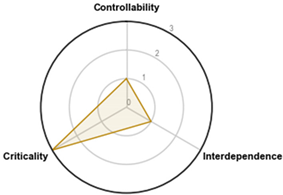 |
| Controllability: State variable dependent | 1 | |
| Criticality: Neutral influence | 3 | |
| Interdependence: Inherent decoupling capabilities | 1 | |
| Overall Score: Moderate suitability | 3 |
Table 7.
Functional Dimension of the identified EFM 1.
| Parameter | Description | |||||
|---|---|---|---|---|---|---|
| System Description | CHW air-conditioning system to supply space cooling. | |||||
| EFM Category | Adaptation of resource allocation | |||||
| Operative Concept | Switching between types of cooling generation units to either increase (↑), by prioritizing the usage of mechanical chillers, or decrease (↓), by prioritizing the usage of the absorption chillers, the electrical demand of the system | |||||
| Adjustment Factor | Ramp-Up and Down of the specific chiller units. | Adjustment Relationship | Step (On/Off) | |||
| MO Amount | MO-1 | Cluster I, ↑ | MO-3 | Cluster II, ↑ | MO Types | Holding |
| MO-2 | Cluster I, ↓ | MO-4 | Cluster II, ↓ | |||
| Execution Level | Supervisory Level | |||||
1 MO: Mode of Operation.
Table 8.
Temporal Dimension of the identified EFM 1.
| Parameter | Value (Min-Max) | Remarks 2 | |||
|---|---|---|---|---|---|
| Active Duration, ∆tActive | 12 min–8 h | Valid for all four MOs | |||
| Planning Duration, ∆tPlanning | 0 | Valid for all four MOs | |||
| Perception Duration, ∆tPerception | 15 min–24 h | Valid for all four MOs | |||
| Decision Duration, ∆tDecision | <1 min | Valid for all four MOs | |||
| Shift Duration, ∆tShift | 5–10 min | Valid for all four MOs | |||
| Activation Duration, ∆tActivation | 10.5 min–24.2 h | Valid for all four MOs | |||
| Deactivation Duration, ∆tDeactivation | 5–10 min | Valid for all four MOs | |||
| Regeneration Duration, ∆tRegeneration | 12 min | Valid for all four MOs | |||
| Validity, V | MO-1 | 69% | MO-3 | 31% | |
| MO-2 | 69% | MO-4 | 31% | ||
| Activation Frequency, NActivation,T | MO-1 | 7092 | MO-3 | 3232 | |
| MO-2 | 7092 | MO-4 | 3232 | ||
1 MO: Mode of Operation. 2 Calculated for Active Duration, ∆tActive, equal to 8 h.
Table 9.
Performance Dimension of the identified EFM.
| Parameter | Value | |||
|---|---|---|---|---|
| Flexibility Type | Bidirectional (↑↓) | |||
| Maximum and Average Flexible Power, ∆Pflex,max (∆Pflex,avg) (kWFlex) | MO-1 | 145.2 (117.2) | MO-3 | 42.9 (25.7) |
| MO-2 | 498.9 (440.3) | MO-4 | 145.2 (117.2) | |
| Flexible Energy Carrier(s) | Electricity/Hot Water (<95 °C) | |||
| Average Flexible Energy 1 Eflex,avg,year (MWhFlex) | MO-1 | 665.1 | MO-3 | 66.5 |
| MO-2 | 2498.7 | MO-4 | 303.3 | |
1 Calculated for Active Duration, ∆tActive, equal to 8 h.
Table 10.
Economic Dimension of the identified EFM.
| Parameter | Value | Description | |||
|---|---|---|---|---|---|
| Investment Costs, Cinvestment | 33,599.25 € | Minor modifications in the system piping and acquisition of new components for the EMS. | |||
| Activation Costs, Cactivation | 0.00 € | No activation costs are considered for the EFM. The costs of each energy carrier are excluded as activation costs as they are used in the net revenue analysis. | |||
| Maintenance Costs, Cmaintenance,T | 53,019.56 € | Due to the added rotation, additional maintenance costs have to be accounted for the chiller units. | |||
| Expected payback period, τpayback | 3 years | Defined by the company based on industry standards for these investments. | |||
| EFM specific cost 1 cflex,T (€/MWhFlex) | MO-1 | 96.6 | MO-3 | 965.6 | Calculated using Equation (4). |
| MO-2 | 25.7 | MO-4 | 211.8 | ||
1 Calculated for Active Duration, ∆tActive, equal to 8 h.
Publisher’s Note: MDPI stays neutral with regard to jurisdictional claims in published maps and institutional affiliations. |
© 2020 by the authors. Licensee MDPI, Basel, Switzerland. This article is an open access article distributed under the terms and conditions of the Creative Commons Attribution (CC BY) license (http://creativecommons.org/licenses/by/4.0/).
Share and Cite
MDPI and ACS Style
Tristán, A.; Heuberger, F.; Sauer, A. A Methodology to Systematically Identify and Characterize Energy Flexibility Measures in Industrial Systems. Energies 2020, 13, 5887. https://doi.org/10.3390/en13225887
AMA Style
Tristán A, Heuberger F, Sauer A. A Methodology to Systematically Identify and Characterize Energy Flexibility Measures in Industrial Systems. Energies. 2020; 13(22):5887. https://doi.org/10.3390/en13225887
Chicago/Turabian StyleTristán, Alejandro, Flurina Heuberger, and Alexander Sauer. 2020. "A Methodology to Systematically Identify and Characterize Energy Flexibility Measures in Industrial Systems" Energies 13, no. 22: 5887. https://doi.org/10.3390/en13225887
Note that from the first issue of 2016, this journal uses article numbers instead of page numbers. See further details here.