A Fuzzy Control Strategy Using the Load Forecast for Air Conditioning System


Tianjin Key Lab of Indoor Air Environmental Quality Control, School of Environmental Science and Engineering, Tianjin University, Tianjin 300072, China
*
Author to whom correspondence should be addressed.
Energies 2020, 13(3), 530; https://doi.org/10.3390/en13030530
Submission received: 9 December 2019
/
Revised: 19 January 2020
/
Accepted: 19 January 2020
/
Published: 21 January 2020
(This article belongs to the Special Issue Evaluation of Energy Efficiency and Flexibility in Smart Buildings)
Abstract
:The energy consumption of air-conditioning systems is a major part of energy consumption in buildings. Optimal control strategies have been increasingly developed in building heating, ventilation, and air-conditioning (HVAC) systems. In this paper, a load forecast fuzzy (LFF) control strategy was proposed. The predictive load based on the SVM method was used as the input parameter of the fuzzy controller to perform feedforward fuzzy control on the HVAC system. This control method was considered as an effective way to reduce energy consumption while ensuring indoor comfort, which can solve the problem of hysteresis and inaccuracy in building HVAC systems by controlling the HVAC system in advance. The case study was conducted on a ground source heat pump system in Tianjin University to validate the proposed control strategy. In addition, the advantages of the LFF control strategy were verified by comparing with two feedback control strategies, which are the supply water temperature (SWT) control strategy and the room temperature fuzzy (RTF) control strategy. Results show that the proposed LFF control strategy is capable not only to ensure the minimum indoor temperature fluctuations but also decrease the total energy consumption.
1. Introduction
Buildings energy systems account for about one-third of the global energy consumption [1]. In China, the total energy consumption of HVAC systems is expected to account for 65% of residential buildings by 2020 [2]. Optimal control strategies have been increasingly developed in building HVAC systems [3]. The energy consumption of building energy systems can be greatly reduced by developing effective control strategies for building HVAC systems [4].
Some scholars have focused on the air-conditioning control strategies. Yordanova et al. [5] designed a fuzzy controller for temperature and humidity control. This method uses fuzzy control to ensure indoor comfort and reduce energy consumption. Wang et al. [6] proposed a direct load control strategy to optimize the distribution of set values for local and global refrigerators by setting adaptive effect functions, which saves energy while ensuring indoor comfort. Krstic [7] proposed a method based on feedback control to compensate for the input delay of any length in a nonlinear control system. Mossolly et al. [8] proposed control strategies based on energy cost and thermal space transient model constraints and they used genetic algorithms to solve problems. This optimization plan/model is suitable for building floor case studies in Beirut. Powell et al. [9] modeled the characteristics of the complexity of large-scale energy systems and used recursive neural networks to accurately predict the hourly load capacity of regional energy systems 24 h in advance. Other researchers have studied the operation and simulation of central air-conditioning systems. Wei et al. [10] obtained the operating power consumption curve based on the mathematical.
Model of the established air conditioning system equipment to determine the optimal operating plan. Chan [11] proposed a solar heating and cooling (SHC) absorption chiller of central air-conditioning system design based on the TRNSYS simulation model for a hotel building. Different control strategies are loaded into the TRNSYS simulation model to evaluate the superiority of different control strategies. Li et al. [12] proposed a central air-conditioning solar heating and cooling (SHC) absorption chiller system based on TRNSYS and proposed three control schemes for the solar collector circuit to determine the preferred design strategy for these systems. Xue et al. [13] proposed a fast power demand response control strategy to investigate the performance of operational dynamics and energy systems in response to strategically controlled demand response events. From the analysis of research status at home and abroad, the current research on control strategies of central air-conditioning systems focuses on the combination of intelligent algorithms and hybrid models. However, the model has insufficient accuracy, inaccurate control, problems such as control errors and overshoot, and overly complex control models are not suitable for actual engineering control.
Judging from the progress of theoretical research at present, although there are many types of research on advanced HVAC system control technology [14,15], the control modes of building HVAC systems presently have a great limitation both in control methods and controlled parameters. From the control method point of view, PID control [16,17,18] is a kind of negative feedback control system, which is widely used in the control of HVAC systems of public buildings by using the proportional integral and differential method to calculate the control amount according to the system deviation. For controlled objects with inherent nonlinearity and hysteresis characteristics [19] such as the HVAC system, it is difficult to obtain an ideal PID control effect due to the uncertainty and time-varying nature of external environmental disturbances. From the controlled parameters point of view, constant pressure control [20] and constant temperature control [21,22] are widely applied. However, there are significant drawbacks to the constant pressure difference and constant temperature difference control of the air conditioning system. On one hand, for constant pressure difference control, there is no direct relationship between the load and pressure difference of the HVAC system. It is not possible to use the differential pressure as a controlled variable to ensure that the chilled water flow changes accurately following the load change [23]. Moreover, the return temperature of the chilled water is inconsistent with the water supply temperature due to the transmission delay of the HVAC system. It is unscientific to adjust the chilled water flow rate according to the temperature difference between the supply and return water detected at the same time as the controlled parameter. Therefore, the control mode based on water supply temperature commonly used for HVAC systems is only applicable to controlled objects or processes without time delay [24,25]. New control techniques and methods need to be adapted to meet the actual needs of the stability and rapid response of the central air conditioning system.
Aiming at the problems existing in HVAC system control technologies, a load forecast fuzzy control strategy was proposed. The predicted load obtained by the SVM method training is used as an input parameter to the controller in advance for feedforward fuzzy control, which can regulate the HVAC system in advance based on the forecast cooling load demand and overcome the shortcomings of controlled parameters. In this study, a simulation platform was established for the heat pump system in Tianjin University based on TRNSYS and MATLAB to confirm the advantages of the proposed LFF control strategy.
2. Case Description
The proposed strategy was validated by an air-conditioning system in Tianjin University Laboratory. The laboratory has two floors and a height of 9 m (see Figure 1). Temperature, humidity sensors, and wind sensors were used for testing. The room temperature measuring point is installed 1 m from the ground level. The central air conditioning system has an automatic platform for monitoring and recording the operating parameters of the air conditioning system. In this case, there are two heat units with a rated cooling capacity of 42 kW and two variable frequency water pumps with a rated power of 3 kW.
The actual operation strategy of the chilled water system is the supply water temperature control strategy, as shown in Figure 2. When the water supply temperature is below the minimum temperature (9 °C), units will be turned on one by one until the temperature rises to the maximum temperature (11 °C). Conversely, when the water temperature is higher than the maximum temperature, units will be turned off one by one until the water temperature is lowered to the minimum temperature. In addition, the unit is equipped with a supercooling protection device, which will shut down all units when the water supply temperature is lower than the minimum temperature for more than one minute. However, in the SWT control strategy, the pump is not controlled.
Another common control strategy is the room temperature fuzzy control strategy. As a feedback control strategy, the control strategy blurs the indoor temperature and the time change rate of the indoor temperature to solve the operation of the control equipment to ensure that the room temperature is controlled at the set value [26]. The control logic diagram of RTF is shown in Figure 3.
3. LFF Control Strategy
Control errors caused by system delay effects may cause adjustment effects to not be reflected in time, resulting in greater overshoot and oscillation. This is a detrimental effect on the air conditioning system control. The objective of the optimal control strategy is to solve the problem of time delay in control, which provides the HVAC system with the capability to operate at relatively high efficiency and save energy at various possible conditions in operation. The proposed LFF control strategy has the following characteristics. The predicted load was obtained based on the SVM [27] method and the predicted load was used as the input parameter of the feed-forward controller. The feed-forward controller can control the HVAC system in advance to eliminate the impact of system time delay on the control of the air conditioning system, and this advanced control time is the time delay of the chilled water transmission of the HVAC system. The predicted load and the time of the advance input are used as input parameters for fuzzy control to obtain control signals for the operation of the water pump and the unit. It is worth mentioning that compared with the SWT control strategy, the LFF control strategy controls the unit while controlling the operation mode of the pump. Compared with the feedback control strategy, the LFF control strategy is load-based feedforward control, which ensures the directness and accuracy of the control.
The control logic diagram of the LFF control strategy is shown in Figure 4. As shown in Figure 4, the cooling load was generated by the weather parameters acting on the building model. Based on the SVM method, the cooling load was trained to obtain the predicted cooling load. The predicted cooling load was applied to the fuzzy controller output control signal u to control the operation of the energy system equipment in advance T.
4. The Method of Control Optimizations
4.1. The Load Forecast Model Based on SVM
Key to the LFF control technology is the accurate input of the cooling load, which determines the effect and quality of control. This paper firstly performs the load simulation calculation on the building model based on TRNSYS, and then the load is predicted by using the support vector machines (SVM) method for the calculated load. SVM is the technique to solve the classification and regression problems [28]. Support vector regression (SVR) is a machine learning method based on statistical learning theory [29].
Support vector machines have strong generalization ability and can effectively solve practical problems such as nonlinearity and small samples. It mainly includes ε-SVR and υ-SVR models [30]. The ε-SVR method maps the input space from a low-dimensional feature space to a high-dimensional feature space based on a nonlinear mapping function φ(x), and then uses Equation (1) to fit a linear function.
In the SVM method, the parameters ω and b are determined using the minimum structural risk. The insensitive loss function parameter ε is introduced to obtain optimization Equations (2)–(5) [31].
The constraints are as follows:
The SVM includes two parameters: the penalty parameter “C” as the intrinsic parameter of SVM and the parameter γ in the kernel function. The penalty parameter “C” and the kernel function γ affect the correlation between the complexity, stability, and vector of the model, respectively. A Gaussian kernel function was introduced to represent the complex non-linear relationship between input and output [32]. The Gaussian kernel function is as follows:
The load of the building was simulated from 15th June to 15th September which is the actual operation period in summer. The meteorological data used in this paper are those of a typical meteorological year.
The flow chart of the SVM method is shown in Figure 5.
The specific steps of load prediction based on the SVM method are as follows.
- The objective function of the support vector machine is established from the training samples. The load calculated by the simulation and the corresponding dry bulb temperature (T, , , ) and wet bulb temperature (W, ) of the typical meteorological year are used as training samples to establish the support vector machine objective function, where , and represent the dry bulb temperatures of 1 h, 2 h, and 3 h in advance and represents the wet bulb temperature 1 h earlier.
- The optimal combination of key parameters of the SVM is determined via MATLAB program calculations. The best combination of key parameters of the SVM is Best c = 14.4149, g = 0.7136.
- The optimal combination parameters are substituted into the SVM model to obtain its decision regression model to obtain the predicted load. The annual (8760 h) maximum instantaneous cooling load obtained by the SVM method is 68.6 kW.
4.2. The Calculation of Time Delay
The time delay of the system includes the heat transfer delay caused by the terminal equipment of the air conditioning system and the time delay caused by the fluid flow of the air conditioning water system. The air conditioning system, in this case, is a fan coil system, and the heat transfer from the terminal to the air is accomplished by convection, which has a small time delay compared to the water system flow and can be ignored [33]. Therefore, only the time delay caused by the flow of the air conditioning water system is considered here.
The time delay of fluid flow, which is the time required for chilled water to flow from the outlet of the air conditioning system to the most unfavorable terminal, can be calculated from the hydraulics of the pipeline. Equation (7) is the ratio of branch pipe flow to total system flow under the assumption that the flow rates at the respective terminal are the same.
The system is assumed to have a total of n branches. The flow rate of each section of the main pipe can be calculated by Equation (8).
The time delay of each main pipe is calculated according to the ratio of the length of the main pipe to the flow rate, which can be computed by Equation (9).
The sum of the time delay of the main sections is the time delay from the outlet of the chilled water to the most unfavorable terminal. The total time delay is calculated as Equation (10). The calculation results are shown in Table 1.
4.3. Fuzzy Control Scheme
A two-dimensional fuzzy controller is established based on the fuzzy logic theory [34] and applied to the HVAC automatic control system. The signal obtained by the sensor is compared with the set value to obtain the deviation e and the deviation change rate ec, and then the deviation e and deviation change rate ec are taken as two inputs of the fuzzy controller. The fuzzy quantization process is performed to obtain the fuzzy variables E and EC. According to fuzzy rules, the fuzzy decision is made to obtain a fuzzy control quantity U. Finally, the actual control output is obtained through the defuzzification and the proportional transformation. For the LFF control strategy, the input of fuzzy control is the cooling load demand. The difference between the input load and the set load is the deviation e. The change rate of the load versus time is the deviation change rate ec. e and ec are the double inputs of the fuzzy control system and the output value u is the pump speed control value.
The sub-fuzzy system was selected to represent the control level. As shown in Equations (11)–(13).
E(e)∈{NB, NM, NS, ZO, PS, PM, PB}
EC(ec)∈{NB, NM, NS, ZO, PS, PM, PB}
U(u)∈{NB, NM, NS, ZO, PS, PM, PB}
E: The universe of E is {−6, −5, −4, −3, −2, −1, 0, 1, 2, 3, 4, 5, 6}. The minimum value of the load is 0 kW and the maximum value is 68.6 kW. In order to convert e into the domain of E, we need to multiply the coefficient ke. The value of ke is determined to be 0.175.
EC: The universe of EC is {−6, −5, −4, −3, −2, −1, 0, 1, 2, 3, 4, 5, 6}. The minimum value of load change rate is −27.2 and the maximum value is 27.2. The universe [−6,6] that converts ec to EC needs to be multiplied by the coefficient kec, the value of kec is determined to be 0.221.
U: The universe of u and U are both [0,1].
Fuzzy sets: Each input parameter is represented by a fuzzy set Ak with a membership function μ, see Equations (14) and (15). The most commonly used triangular membership function was used in this study [35].
Ak = {(i, μ(i)}
μ(i)∈[0,1]
4.4. Optimization of Pumps and Units Control
The control strategy of the pump is as follows: when the required flow of the system is less than or equal to half of the maximum flow, one pump is individually frequency-controlled and the other is not operated. If the required flow is greater than half of the maximum flow, one pump provides half the flow at full load and the other pump provides the remaining flow by frequency conversion. Specific control strategies for pumps is shown in Table 2. The fuzzy control output value u is between 0 and 1. The pump operates at a frequency and the operating frequency is proportional to the control signal.
In order to ensure the normal operation of the system, one unit is always running and the other unit is controlled by the set start-stop time. The start and stop time means that the unit is turned on within the set time, while the unit is turned off outside the set time. For example, a start-stop time of 0.5 means that the unit’s on-time and off-time are each half of the total operating time. The specific operation control strategy of the unit is shown in Table 3.
5. TRNSYS Simulation Platform
5.1. Establishment of the Simulation Platform
The construction of the test platform based on TRNSYS is shown in Figure 6. In this case, the simulation time is from 15th June to 15th September of the typical meteorological year, for a total of 2231 h. The building is simulated by a single area building module (Type 12) in TRNSYS. A water-water heat pump system is used in this case. Type 668 was selected as the water-water heat pump unit module. The cooling transmission in the system is achieved by the variable speed pump module Type 110. In order to advance the predicted load in advance and consider the delay caused by the flow of the central air conditioning chilled water system, the delay module (Type 93) is added to the test platform. The model is closer to the actual system and lays the foundation for subsequent feedforward control. In the test platform, the switch differential controller Type 2 and the Type 155 read the chilled water supply temperature of the heat pump unit and collectively control the heat pump unit operation to make it the same as the actual operation logic.
5.2. Verification of Simulation Platform
5.2.1. Indoor Temperature Validation Test
Based on the actual monitoring data, the weather data measured from 6th August to 11th August, 2017 were selected to verify the system simulation model. In order to reduce the influence of the initial conditions on the simulation, the actual indoor temperature on 8th August when the system is on stable operation is compared with the indoor simulated temperature with and without considering the delay effect of the system respectively. The temperature comparison results are shown in Figure 7. It can be seen from Figure 7 that the indoor temperature curve obtained by the simulation platform with delay effect is basically consistent with the actual temperature curve during the period from 9 am to 8 pm. The maximum temperature difference at a single point is 0.8 °C, and the average relative temperature difference is 0.4 °C. However, there is a large deviation between the actual room temperature and the indoor simulation temperature without considering the system delay effect. The maximum single point temperature difference is 1.9 °C, and the average relative temperature difference is 1.1 °C. As a result of this, in the simulation of the room temperature, the model considering the delay effect of the system is more in line with the actual situation. In the period from 1 am to 9 am, the reason for the error in the simulation result of the model considering the system delay effect is that the unit was set to be completely closed when the chilled water outlet temperature is lower than 8 °C in the simulation model in order to reduce the frequent oscillation of the system parameters during the simulation. This will result in a lower temperature of the chilled water at night, which in turn will result in lower room temperature. The simulated temperature from 4 pm to 7 pm is also low because the simplified room model only considers the effect of outdoor temperature on the indoor load and does not consider the effects of radiation. The indoor load was influenced by solar radiation and the heat storage effect of the wall, which leads to increased room temperature.
5.2.2. Heat Pump Unit and Pump Energy Consumption Validation Test
The energy consumption of the heat pump unit for the actual three hours based on the load rate and power of the heat pump unit during three time periods were monitored and calculated, from 9:22 to 10:22 on 7th August, 15:03 to 16:03 on 8th August, and from 13:17 to 14:17 on 11th August.
As shown in Figure 8, within three test days, the energy consumption of the heat pump unit under the consideration of time delay, without considering time delay, and actual control conditions have been marked, which shows the comparison of energy consumption within 3 h for the model unit considering the system delay effect, without considering the system delay effect, and the actual unit, respectively. It can be seen that the relative errors of the total energy consumption of the actual unit and the simulated total energy consumption of the unit with and without considering the system delay effect are 4.0% and 14.4%. This shows that a system with a delay effect is more energy-efficient than a system without a delay effect because the cooling load is input at an early time. From the above, the simulated energy consumption of the heat pump unit considering the system delay effect is more consistent with the actual energy consumption.
The two pumps have been operating at full load, with a rated power of each pump at 3 kW. Therefore, the water pump energy consumption per hour is 6 kWh, and the actual total energy consumption of the three-hour pump is 18 kWh. Figure 9 shows the comparison of the system with and without the delay module, and the actual unit pumps energy consumption within three hours. The relative error between the actual total pump energy consumption and the simulated total energy consumption of the pump considering the delay effect of the system is 0.2%, without considering the delay effect of the system is 1.1%. The reason why the difference between both models is small is that the pump operates at a fixed frequency. Since the pump runs at a fixed frequency, the control signal cannot be controlled by the variable frequency like the control unit, and the energy consumption of the pump can only be reduced by changing the start and stop time of the pump. Therefore, the energy consumption of the system pump with or without delay effect is basically the same.
6. Results and Discussion
Based on the test platform, the indoor temperature and total system energy consumption under the three control strategies (LFF, RTF, and SWT) were simulated. The TRNSYS simulation platform of the LFF control strategy is shown in Figure 10.
6.1. Simulation Results of Indoor Temperature
The room temperatures of the three control strategies were compared under both full-time simulation and hottest day simulation conditions. The temperature results of LFF, RTF, and SWT control strategies for the full-time simulation correspond to Figure 11a–c, respectively. As can be seen from Figure 11, three control strategies can control the room temperature between 25 °C and 27 °C when the air conditioning system is in operation. Indoor temperatures above 27 °C occur at night when the outdoor temperature is high.
During the entire simulation, the outdoor temperature was the highest on 19th June, so the simulation results of 19th June were selected to analyze the indoor temperature control of the HVAC system under the limit conditions. The room temperature comparison under different control strategies on 19th June is shown in Figure 12.
All three control strategies can control the room temperature within the operating period of the air conditioning system between 25 °C and 27 °C. Three kinds of control of the temperature range are acceptable. During the 0:00 to 7:00 and 20:00 to 23:00 periods which the air-conditioning chilled water system is not in operation, the indoor room temperature under the three control strategies is almost the same regardless of the trend or value. However, in the period of 7:00 to 20:00 when the air-conditioning chilled water system is in operation, there are obvious differences in the indoor room temperature control effect under the three control strategies. The room temperature under SWT control fluctuates the most. The room temperature reaches a maximum of 27 °C at 10:00. At this time, the temperature of the external wall will rise due to the increase of the outdoor temperature, thus making the indoor temperature rise. The room temperature reached a minimum of 25 °C at 19:00 because the chilled water temperature of the unit was turned off at 8 °C, which in turn caused the indoor temperature to drop. The room temperature under the RTF control fluctuated relatively less with a fluctuation range of 25.4 °C and 26.8 °C. The RTF control strategy is based on the indoor temperature as the control object, and the fuzzy temperature of the set temperature range is solved to ensure the thermal comfort of the indoor temperature. However, with the LFF control strategy of predictive load feed-forward control, the required load of the system is given from the demand-side response, which can ensure that the system operating temperature just matches the room temperature demand. Therefore, the room temperature fluctuation range under the LFF control strategy is between 25.4 °C and 26.4 °C, and among the three control strategies, the temperature fluctuation range is the smallest.
6.2. Simulation Results of Energy Consumption
The total hourly energy consumption of pumps and units under all three control strategies are shown in Figure 13.
The comparison of energy consumption under the three control strategies for the system is shown in Figure 14. It can be intuitively seen from Figure 14 that the LFF control strategy consumes the least amount of energy, whether it is the total energy consumption of the system or the energy consumption of the unit and the pump. The energy consumption of the system under the LFF control strategy is the least because the system is controlled from the demand- side, the system is feed-forward input according to the predicted load advance time delay, and the operation of the pumps and units is fuzzy controlled. Demand-side control can fundamentally solve problems such as the mismatch between system energy consumption and required cooling capacity, and avoid unnecessary startup and overload operation of the unit. Compared with the LFF control strategy, the RTF control strategy, as a feedback control, has a significantly better control effect than the actual control strategy based on the temperature difference between the supply and return water. However, due to problems such as time delay in feedback control, it is impossible to determine the operation of the system from the demand-side feedforward control, which will cause certain unnecessary energy loss in the system. Table 4 shows the energy consumption comparison between LFF and the other two control strategies (SWT, RTF), respectively. Compared to the SWT control strategy, the LFF control strategy has a heat pump unit energy-saving rate of 14.5%, a pump energy-saving rate of 10.2%, and a total energy-saving rate of 13.4%. Compared with the RTF control strategy, the LFF control strategy has a relatively low energy-saving rate of 9.2%, 4.1%, and 7.8%, respectively.
7. Conclusions
In order to solve the problem of time delay in the control process of the air conditioning system, the LFF control strategy was developed. In this control strategy, the cooling load forecast is used as an input parameter to regulate and control the air conditioning system in advance and ignore the problem of parameter variation caused by time delay in the control process.
The energy performance under the LFF control strategy has been validated based on the actual case built TRNSYS simulation platform. The results show that compared with the commonly used feedback control strategy, the proposed effective control concept ensures indoor comfort and reduces system energy consumption. Under the LFF control, the indoor temperature fluctuations are minimal and the energy consumption under this control strategy is the lowest. Compared with the SWT and RTF controls, the total energy consumption of the LFF control at full-time simulation was reduced by 13.4% and 7.8%, respectively.
However, the simulation analysis results of the energy-saving rate have some limitations. By changing the simulation parameters, it can be found that the system energy-saving rate obtained by the TRNSYS simulation platform is mainly affected by outdoor meteorological parameters and thermal performance parameters of the building envelope. For different types of buildings and different outdoor meteorological parameters, the system energy-saving rates simulated by the LFF control strategy are often different.
Author Contributions
Methodology, J.Z.; software, R.G.; Y.S.; validation, Y.S. formal analysis, J.Z.; investigation, J.Z.; R.G.; resources, J.Z.; writing—original draft preparation, Y.S.; writing—review and editing, Y.S.; R.G. All authors have read and agreed to the published version of the manuscript.
Funding
This research was supported by the Natural Science Foundation of China, Project No. 51678398 and the Natural Science Foundation of Tianjin, Project No.18JCQNJC08400. “The funders had no role in the design of the study; in the collection, analyses, or interpretation of data; in the writing of the manuscript, or in the decision to publish the results”.
Conflicts of Interest
The authors declare no conflict of interest.
Nomenclature
| LFF | load forecast fuzzy |
| RTF | room temperature fuzzy |
| SWT | supply water temperature |
| SVM | Support Vector Machines |
| SVR | Support Vector Regression |
| C | error cost |
| γ | kernel parameter |
| the number of the terminal of the branch I of the air conditioning system | |
| the ratio of the flow rate of each branch pipe to the total flow | |
| Dn | the inner diameter of the chilled water outlet pipe |
| the delay time of each main pipe | |
| NB | negative large |
| NS | negative small |
| PS | positive small |
| PB | positive large |
| Ak | fuzzy set |
| EC | the change rate of the load versus time |
| ω | weight vectors |
| nonlinear mapping function | |
| threshold | |
| (xm, ym) | a pair of input and output vectors |
| n | number of samples |
| upper training error | |
| lower training error | |
| M | the total number of the terminal of the air conditioning system |
| he inner diameter of each section of the main pipe | |
| he real-time flow rate of the chilled water outlet. | |
| the length of each main pipe | |
| NM | medium |
| Z | zero |
| PM | medium |
| μ | a membership function |
| E | the difference between the input load and the set load |
| U | Pump speed control |
References
- Costa, A.; Keane, M.M.; Torrens, J.I.; Corry, E. Building operation and energy performance: Monitoring, analysis and optimisation toolkit. Appl. Energy 2013, 101, 310–316. [Google Scholar] [CrossRef]
- Lam, J.C.; Wan, K.K.; Tsang, C.L.; Yang, L. Building energy efficiency in different cli-mates. Energy Convers Manag. 2008, 49, 2354–2366. [Google Scholar] [CrossRef]
- Du, Z.M.; Jin, X.Q.; Fang, X.; Fan, B. A dual-benchmark based energy analysis method to evaluate control strategies for building HVAC systems. Appl. Energy 2016, 183, 700–714. [Google Scholar] [CrossRef]
- Peng, Y.; Rysanek, A.; Nagy, Z. Using machine learning techniques for occupancy-prediction-based cooling control in office buildings. Appl. Energy 2018, 211, 1343–1358. [Google Scholar] [CrossRef]
- Yordanova, S.; Merazchiev, D.; Jain, L. A Two-Variable Fuzzy Control Design with Application to an Air-Conditioning System. Fuzzy Syst. IEEE Trans. 2015, 23, 474–481. [Google Scholar] [CrossRef]
- Wang, S.W.; Tang, R. Supply-based feedback control strategy of air-conditioning systems for direct load control of buildings responding to urgent requests of smart grids. Appl. Energy 2017, 201, 419–432. [Google Scholar] [CrossRef]
- Krstic, M. Input Delay Compensation for Forward Complete and Strict-Feedforward Nonlinear Systems. IEEE Trans. Autom. Control 2010, 55, 287–303. [Google Scholar] [CrossRef]
- Mossolly, M.; Ghali, K.; Ghaddar, N. Optimal control strategy for a multi-zone air conditioning system using a genetic algorithm. Energy 2009, 34, 58–66. [Google Scholar] [CrossRef]
- Powell, K.M.; Sriprasad, A.; Cole, W.J.; Edgar, T.F. Heating, cooling, and electrical load forecasting for a large-scale district energy system. Energy 2014, 74, 877–885. [Google Scholar] [CrossRef]
- Wei, B.; Tang, J.; Wei, Z. Dynamic simulation to the operation of central air conditioning system. Ind. Electron. Appl. 2010, 100, 861–867. [Google Scholar]
- Chan, I.Y.T. Simulation and evaluation of control strategies for air conditioning system using TRNSYS. Int. J. Prison. Health 2012, 8, 92–99. [Google Scholar]
- Li, Q.; Zheng, C.; Shirazi, A.; Mousa, O.B.; Moscia, F.; Scottc, J.A.; Taylor, R.A. Design and analysis of a medium-temperature, concentrated solar thermal collector for air-conditioning applications. Appl. Energy 2017, 190, 1159–1173. [Google Scholar] [CrossRef]
- Xue, X.; Wang, S.; Yan, C.; Cui, B. A fast chiller power demand response control strategy for buildings connected to smart grid. Appl. Energy 2015, 137, 77–87. [Google Scholar] [CrossRef]
- Shirazi, A.; Pintaldi, S.; White, S.D.; Morrison, G.L.; Rosengarten, G.; Tylor, R.A. Solar-assisted absorption air-conditioning systems in buildings: Control strategies and operational modes. Appl. Therm. Eng. 2016, 92, 246–260. [Google Scholar] [CrossRef]
- Fiorentini, M.; Wall, J.; Ma, Z.; Braslavsky, J.H.; Cooper, P. Hybrid model predictive control of a residential HVAC system with on-site thermal energy generation and storage. Appl. Energy 2017, 187, 465–479. [Google Scholar] [CrossRef] [Green Version]
- Attaran, S.M.; Yusof, R.; Selamat, H. A novel optimization algorithm based on epsilon constraint-RBF neural network for tuning PID controller in decoupled HVAC system. Appl. Therm. Eng. 2016, 99, 613–624. [Google Scholar] [CrossRef]
- Lygouras, J.N.; Botsaris, P.N.; Vourvoulakis, J.; Kodogiannis, V. Fuzzy logic controller implementation for a solar air-conditioning system. Appl. Energy 2007, 84, 1305–1318. [Google Scholar] [CrossRef]
- Wang, J.J.; An, D.W.; Jing, Y.Y. Genetic optimization algorithm of PID decoupling control for VAV air-conditioning system. J. Tianjin Univ. 2009, 15, 308–314. [Google Scholar] [CrossRef]
- Xia, Y.; Deng, S.; Chen, M.Y. Inherent operational characteristics and operational stability of a variable speed direct expansion air conditioning system. Appl. Therm. Eng. 2016, 73, 268–277. [Google Scholar] [CrossRef]
- Li, X.; Chen, J.; Chen, Z.; Liu, W.; Hu, W. A new method for controlling refrigerant flow in automobile air conditioning. Appl. Therm. Eng. 2004, 24, 1073–1085. [Google Scholar] [CrossRef]
- Li, S. Optimum Control Strategy and Performance Simulation of a Constant Temperature and Humidity Air-conditioning System. J. Refrig. 2012, 33, 22–27. [Google Scholar]
- Yu, X.; Wang, R.Z.; Zhai, X.Q. Year round experimental study on a constant temperature and humidity air-conditioning system driven by ground source heat pump. Energy 2011, 36, 1309–1318. [Google Scholar] [CrossRef]
- Liu, X.; Liu, J.; Lu, Z.; Xing, K.; Mai, Y. Diversity of energy-saving control strategy for a parallel chilled water pump based on variable differential pressure control in an air-conditioning system. Energy 2015, 88, 718–733. [Google Scholar]
- Liu, X.F.; Liu, J.P.; Lu, J.D.; Liu, L.; Zou, W. Research on operating characteristics of direct-return chilled water system controlled by variable temperature difference. Energy 2012, 40, 236–249. [Google Scholar] [CrossRef]
- Wang, S.; Gao, D.C.; Sun, Y.; Xiao, F. An online adaptive optimal control strategy for complex building chilled water systems involving intermediate heat exchangers. Appl. Therm. Eng. 2013, 50, 614–628. [Google Scholar] [CrossRef]
- Chiou, C.B.; Chiou, C.H.; Chu, C.M.; Lin, S.L. The application of fuzzy control on energy saving for multi-unit room air-conditioners. Appl. Therm. Eng. 2009, 29, 310–316. [Google Scholar] [CrossRef]
- Cortes, C.; Vapnik, V.N. Support vector networks. Mach. Learn. 1995, 20, 273–295. [Google Scholar] [CrossRef]
- Selakov, A.; Cvijetinović, D.; Milović, L. Hybrid PSO-SVM method for short-term load forecasting during periods with significant temperature variations in city of Burbank. Appl. Soft Comput. 2014, 16, 80–88. [Google Scholar] [CrossRef]
- Awad, M.; Khanna, R. Support Vector Regression. Neural Inf. Process. Lett. Rev. 2007, 11, 203–224. [Google Scholar]
- Fu, Y.; Li, Z.; Zhang, H. Using Support vector machine to predict next-day electricity load of public buildings with sub-metering devices. Procedia Eng. 2015, 121, 1016–1022. [Google Scholar] [CrossRef] [Green Version]
- Shrivastava, N.A.; Khosravi, A.; Panigrahi, B.K. Prediction Interval Estimation of Electricity Prices Using PSO-Tuned Support Vector Machines. IEEE Trans. Ind. Inform. 2015, 11, 322–331. [Google Scholar] [CrossRef]
- Ebtehaj, I.; Bonakdari, H.; Shamshirband, S. A combined support vector machine-wavelet transform model for prediction of sediment transport in sewer. Flow Meas. Instrum. 2016, 47, 19–27. [Google Scholar] [CrossRef]
- Li, Y.M.; Wu, J.Y.; Shiochi, S. Experimental validation of the simulation module of the water-cooled variable refrigerant flow system under cooling operation. Appl. Energy 2010, 87, 1513–1521. [Google Scholar] [CrossRef]
- Hien, L.V.; Trinh, H. Stability Analysis and Control of Two-Dimensional Fuzzy Systems with Directional Time-Varying Delays. IEEE Trans. Fuzzy Syst. 2018, 26, 1550–1564. [Google Scholar] [CrossRef]
- Ozkop, E.; Altas, I.H.; Okumus, H.I.; Sharaf, A.M. A fuzzy logic sliding mode controlled electronic differential for a direct wheel drive EV. Int. J. Electron. 2015, 102, 1919–1942. [Google Scholar] [CrossRef]
Figure 1.
Lab Exterior View.

Figure 2.
The logic diagram of the supply water temperature (SWT) control strategy.
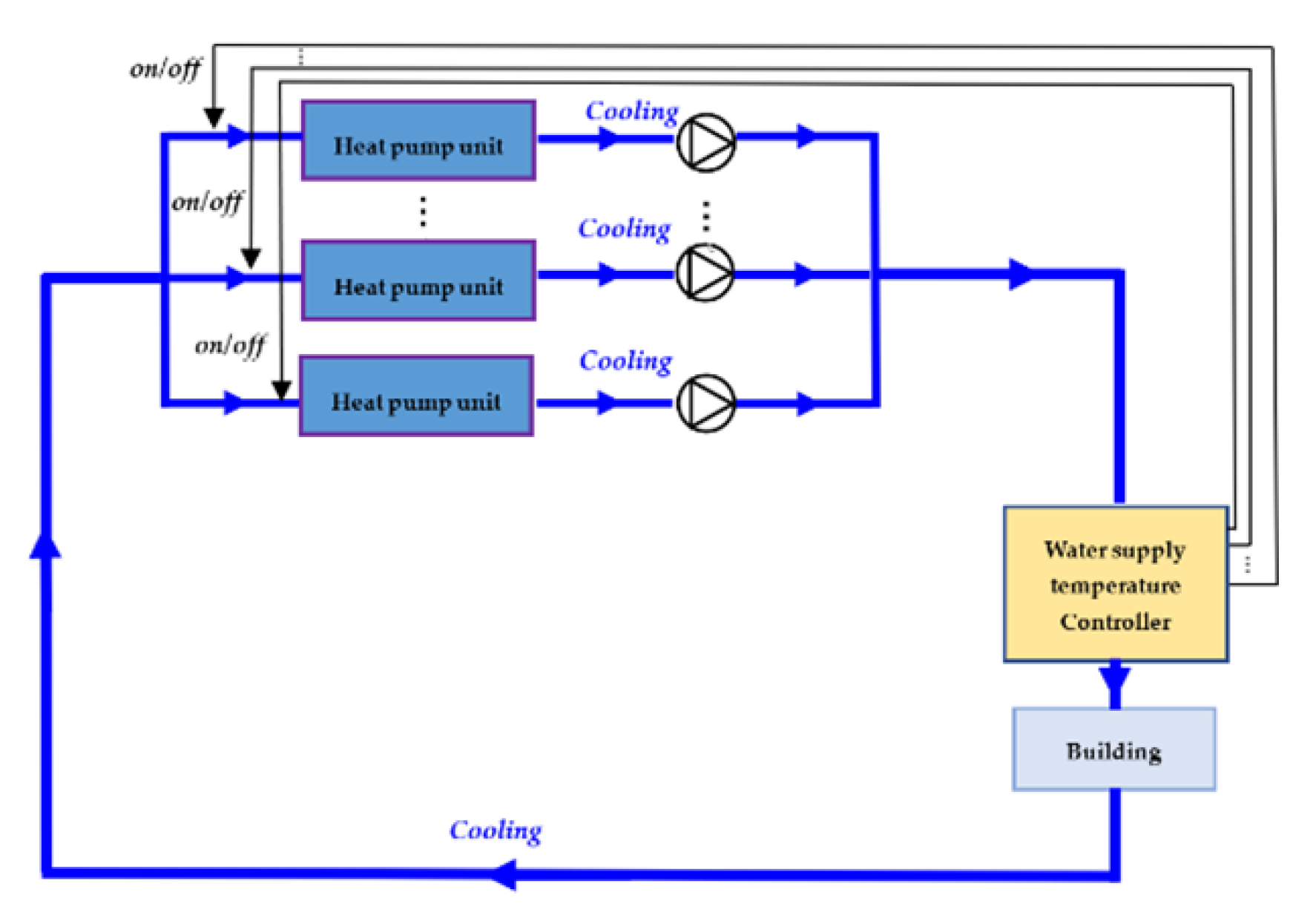
Figure 3.
The logic diagram of the room temperature fuzzy (RTF) control strategy.

Figure 4.
The logic diagram of the load forecast fuzzy (LFF) control strategy.

Figure 5.
The flow chart of the support vector machines (SVM) method.

Figure 6.
TRNSYS simulation platform.

Figure 7.
The temperature in three modes.

Figure 8.
Comparison of simulated energy consumption and actual energy consumption of heat pump units.
Figure 8.
Comparison of simulated energy consumption and actual energy consumption of heat pump units.

Figure 9.
Comparison between simulated energy consumption and actual energy consumption of water pumps.
Figure 9.
Comparison between simulated energy consumption and actual energy consumption of water pumps.
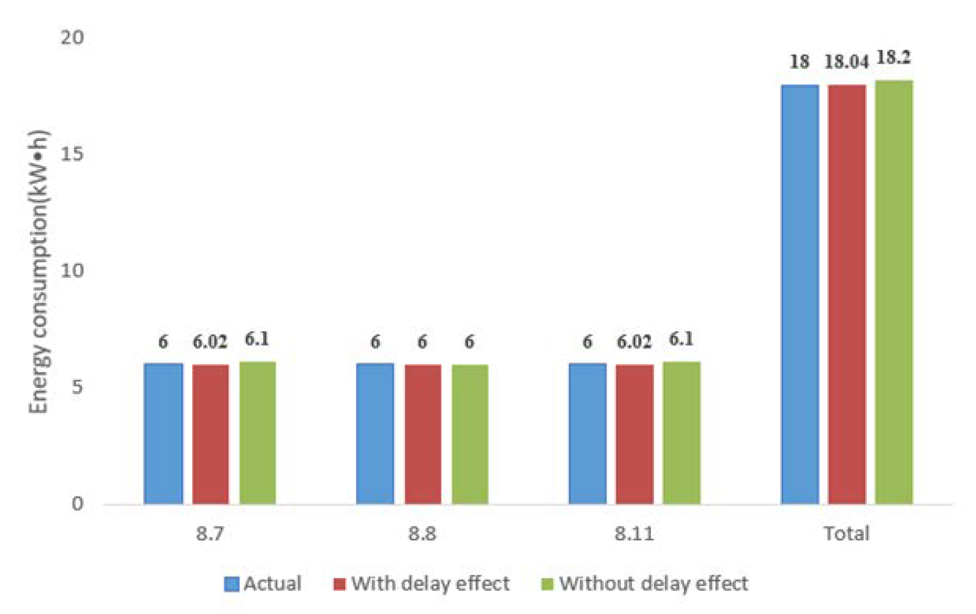
Figure 10.
TRNSYS simulation platform of the LFF control strategy.
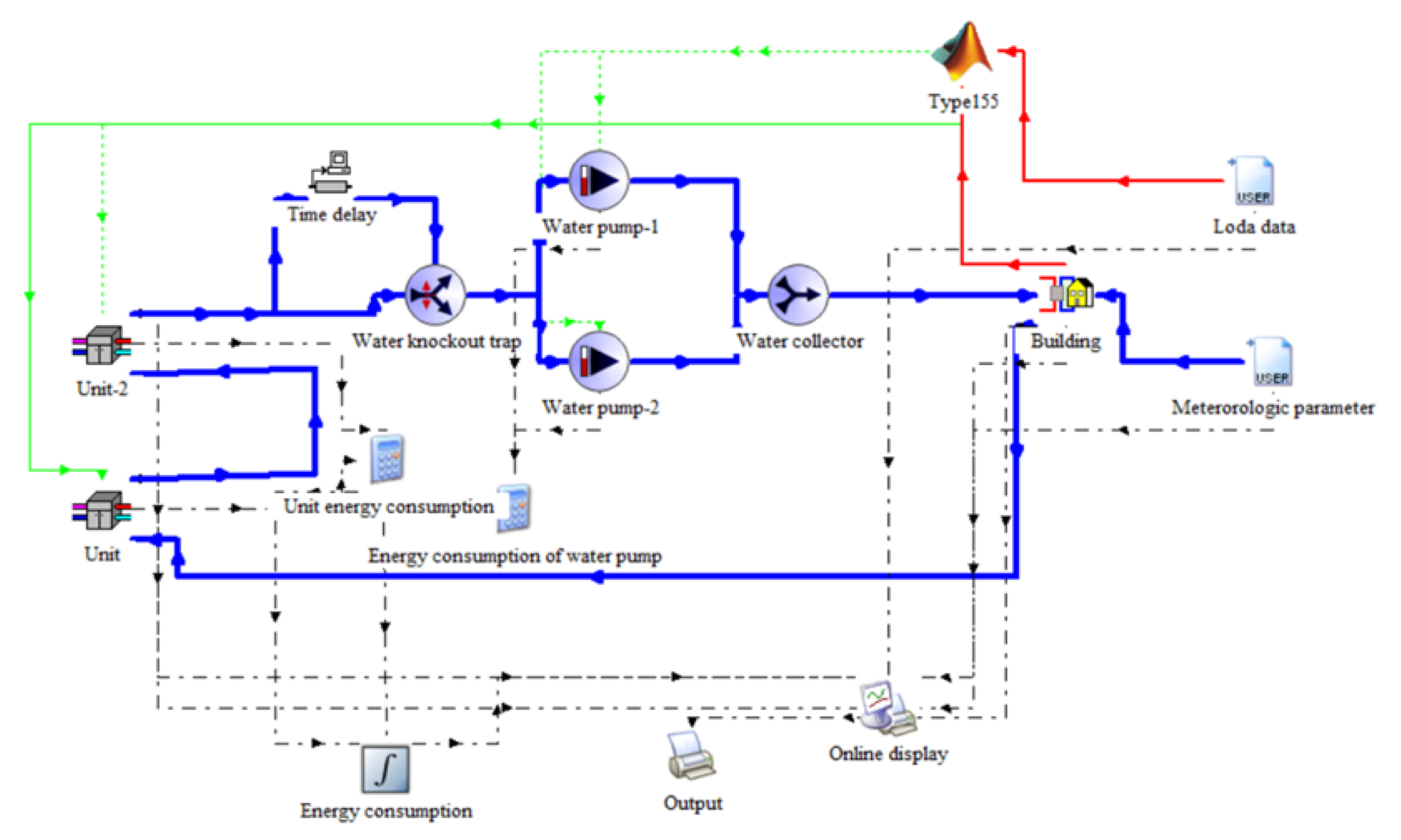
Figure 11.
(a) Room temperature simulation results under LFF control; (b) Room temperature simulation results under RTF control; (c) Room temperature simulation results under SWT control.
Figure 11.
(a) Room temperature simulation results under LFF control; (b) Room temperature simulation results under RTF control; (c) Room temperature simulation results under SWT control.
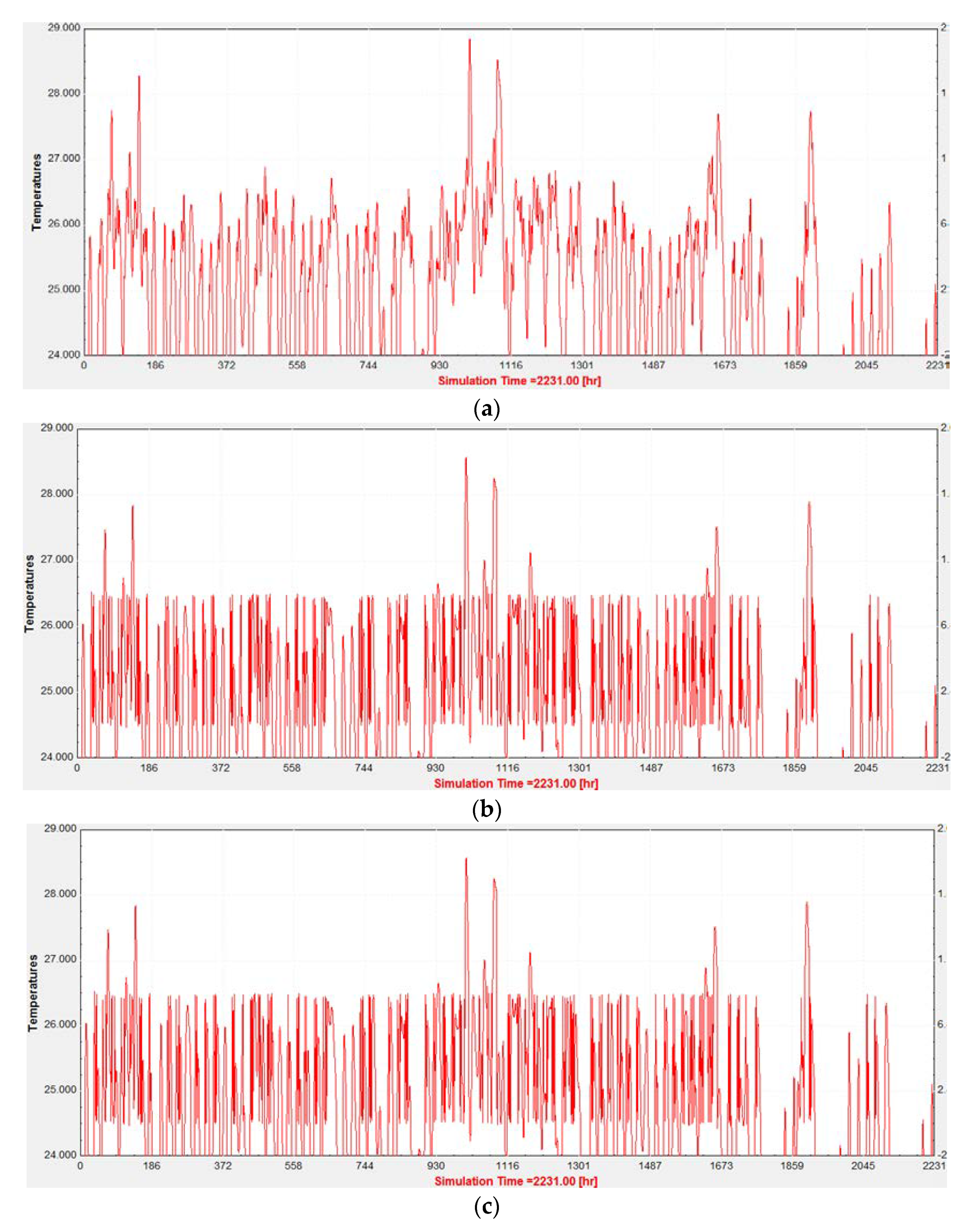
Figure 12.
Comparison of room temperature under different control strategies on 19th June.

Figure 13.
The simulation results of energy consumption under three different control strategy.

Figure 14.
Comparison of energy consumption under three conditions.


Table 1.
The theoretical calculation of the time delay caused by the flow.
| 1 | 5.30 | 32 | 1/12 | 0.12 | 44.24 |
| 2 | 7.24 | 40 | 1/12 | 0.15 | 47.22 |
| 3 | 4.41 | 50 | 1/12 | 0.15 | 29.96 |
| 4 | 7.32 | 50 | 1/12 | 0.20 | 37.30 |
| 5 | 8.01 | 50 | 1/12 | 0.25 | 32.65 |
| 6 | 5.45 | 65 | 1/12 | 0.17 | 31.29 |
| 7 | 6.80 | 65 | 1/12 | 0.20 | 33.46 |
| 8 | 4.69 | 65 | 1/12 | 0.23 | 20.19 |
| 9 | 8.52 | 65 | 1/12 | 0.26 | 32.61 |
| 10 | 7.21 | 80 | 1/12 | 0.19 | 37.62 |
| 11 | 4.69 | 80 | 1/12 | 0.21 | 22.25 |
| 12 | 16.4 | 80 | 1/12 | 0.23 | 71.30 |
| Total | 440 | ||||
Table 2.
Pump control strategy.
| u | Pump Control Method |
|---|---|
| 0.0–0.2 | Both pumps are off and the pump control signal is 0 |
| 0.2–0.5 | One pump control signal is 0, the other pump control signal is 0.5 + u |
| 0.5–1.0 | One pump control signal is 1 and the other control signal is 2u − 1 |
Table 3.
Heat units control strategy.
| u | Heat Units Control Method |
|---|---|
| 0.00–0.50 | One unit start-stop time ratio is 1, another unit start-stop time ratio is 0 |
| 0.50–0.66 | One unit start-stop time ratio is 1, another unit start-stop time ratio is 0.17 |
| 0.66–0.75 | One unit start-stop time ratio is 1, another unit start-stop time ratio is 0.33 |
| 0.75–0.80 | One unit start-stop time ratio is 1, another unit start-stop time ratio is 0.50 |
| 0.80–1.00 | Start and stop time rate of both units is 1 |
Table 4.
Comparison of energy-saving rates of LFF control strategies compared to the other two control strategies.
Table 4.
Comparison of energy-saving rates of LFF control strategies compared to the other two control strategies.
| Contrast Item | Unit Energy Consumption (kW·h)/Energy Saving Rate (%) | Pump Energy Consumption (kW·h)/Energy Saving Rate (%) | Total Energy Consumption (kW·h)/Energy Saving Rate (%) |
|---|---|---|---|
| LFF | 4016 | 1740 | 5756 |
| SWT | 4713/14.5% | 1937/10.2% | 6650/13.4% |
| RTF | 4425/9.2% | 1815/4.1% | 6240/7.8% |
© 2020 by the authors. Licensee MDPI, Basel, Switzerland. This article is an open access article distributed under the terms and conditions of the Creative Commons Attribution (CC BY) license (http://creativecommons.org/licenses/by/4.0/).
Share and Cite
MDPI and ACS Style
Zhao, J.; Shan, Y. A Fuzzy Control Strategy Using the Load Forecast for Air Conditioning System. Energies 2020, 13, 530. https://doi.org/10.3390/en13030530
AMA Style
Zhao J, Shan Y. A Fuzzy Control Strategy Using the Load Forecast for Air Conditioning System. Energies. 2020; 13(3):530. https://doi.org/10.3390/en13030530
Chicago/Turabian StyleZhao, Jing, and Yu Shan. 2020. "A Fuzzy Control Strategy Using the Load Forecast for Air Conditioning System" Energies 13, no. 3: 530. https://doi.org/10.3390/en13030530
Note that from the first issue of 2016, this journal uses article numbers instead of page numbers. See further details here.