Evaluation of Energy Efficiency and the Reduction of Atmospheric Emissions by Generating Electricity from a Solar Thermal Power Generation Plant


Abstract
:
1. Introduction
2. Materials and Methods
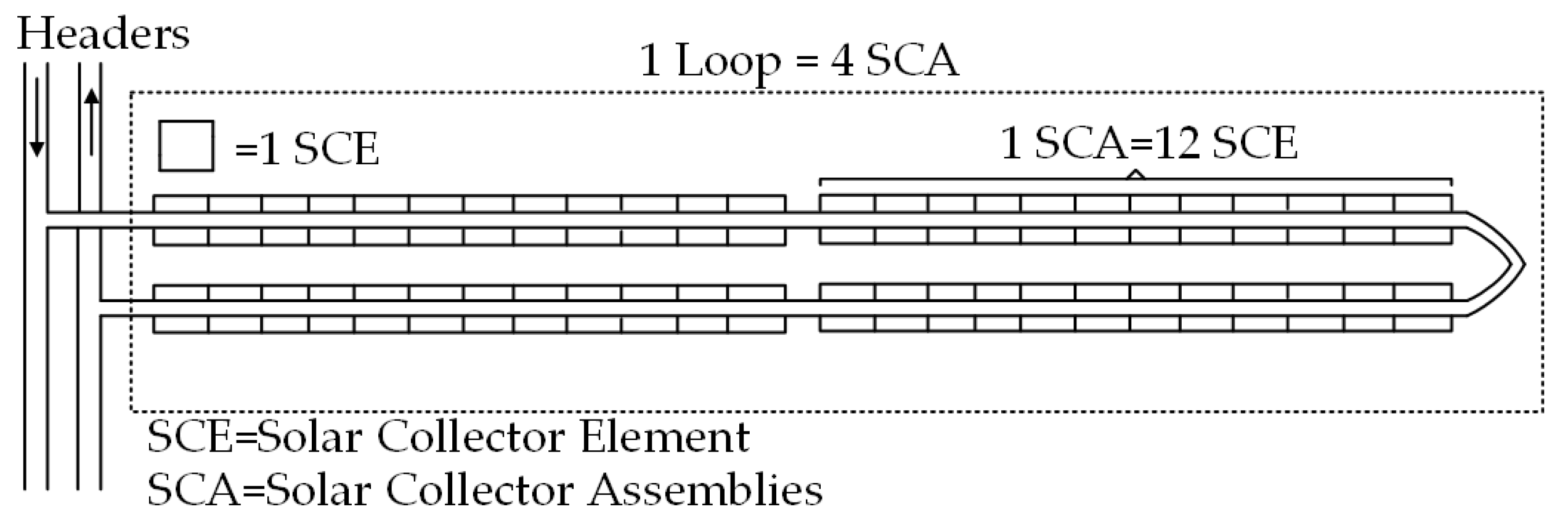
2.1. Solar Collector Field
Parameter Model
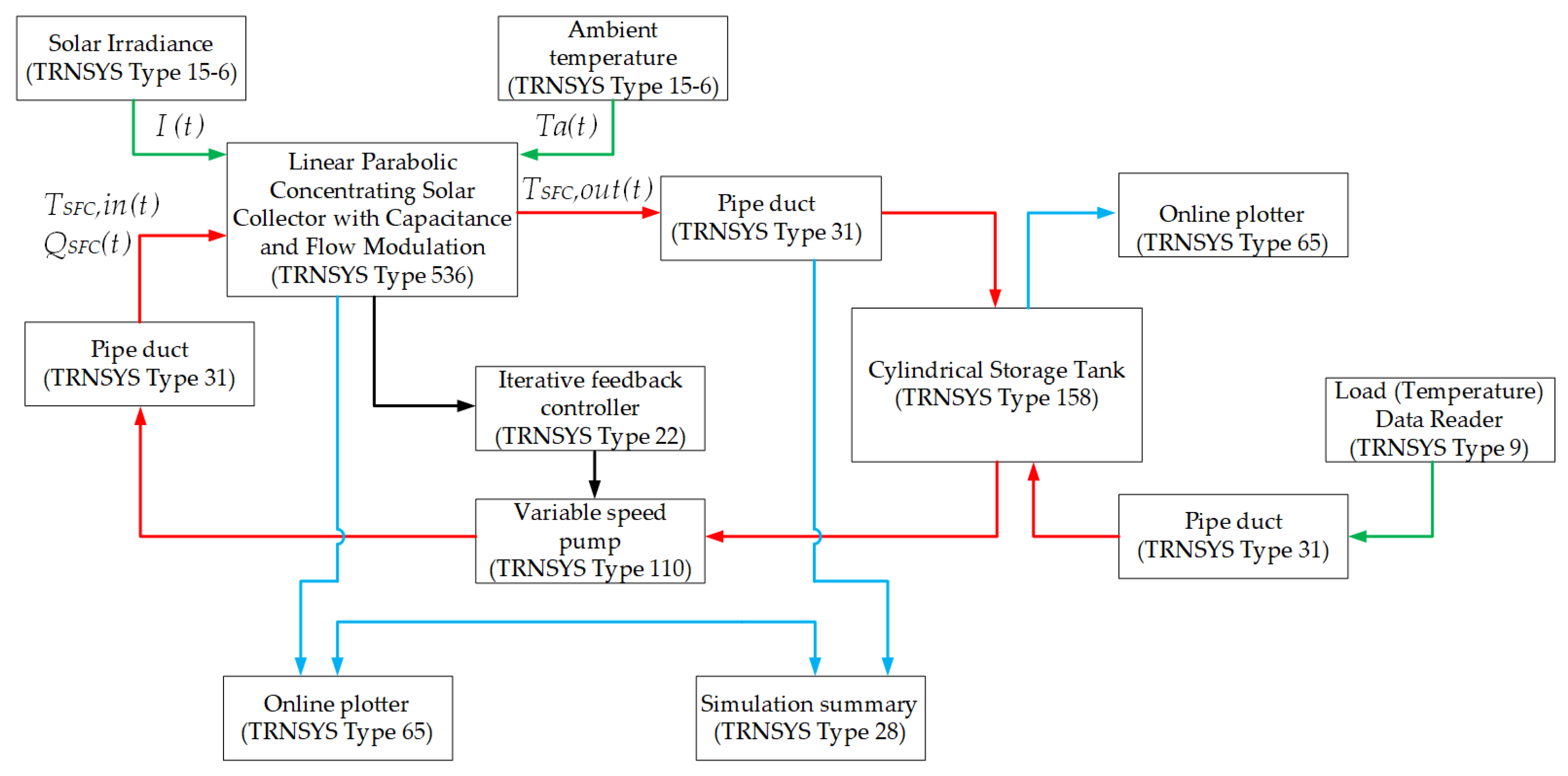
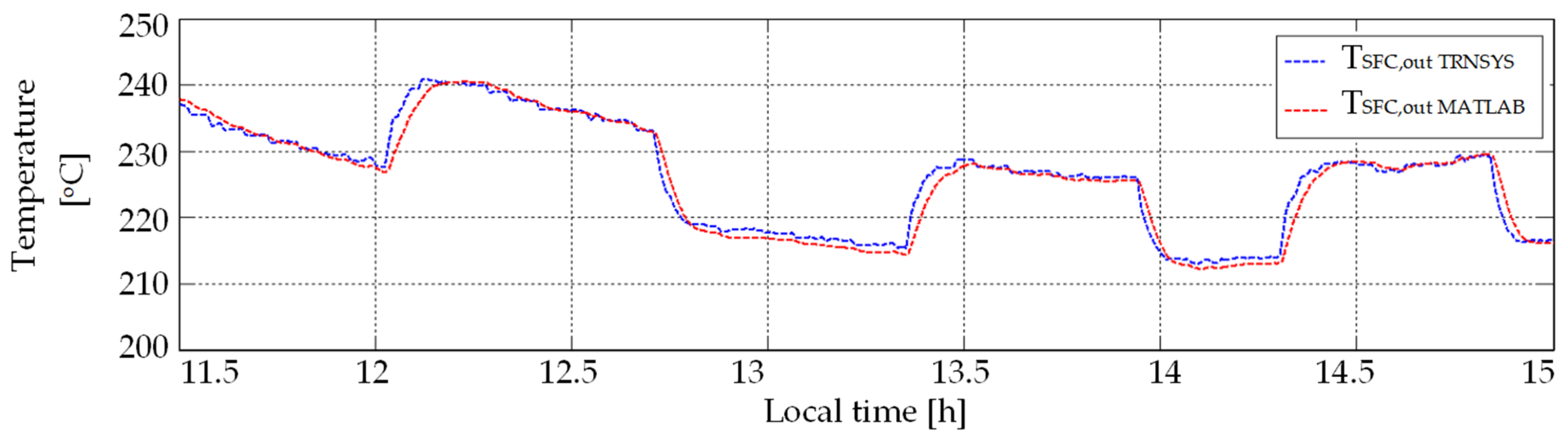
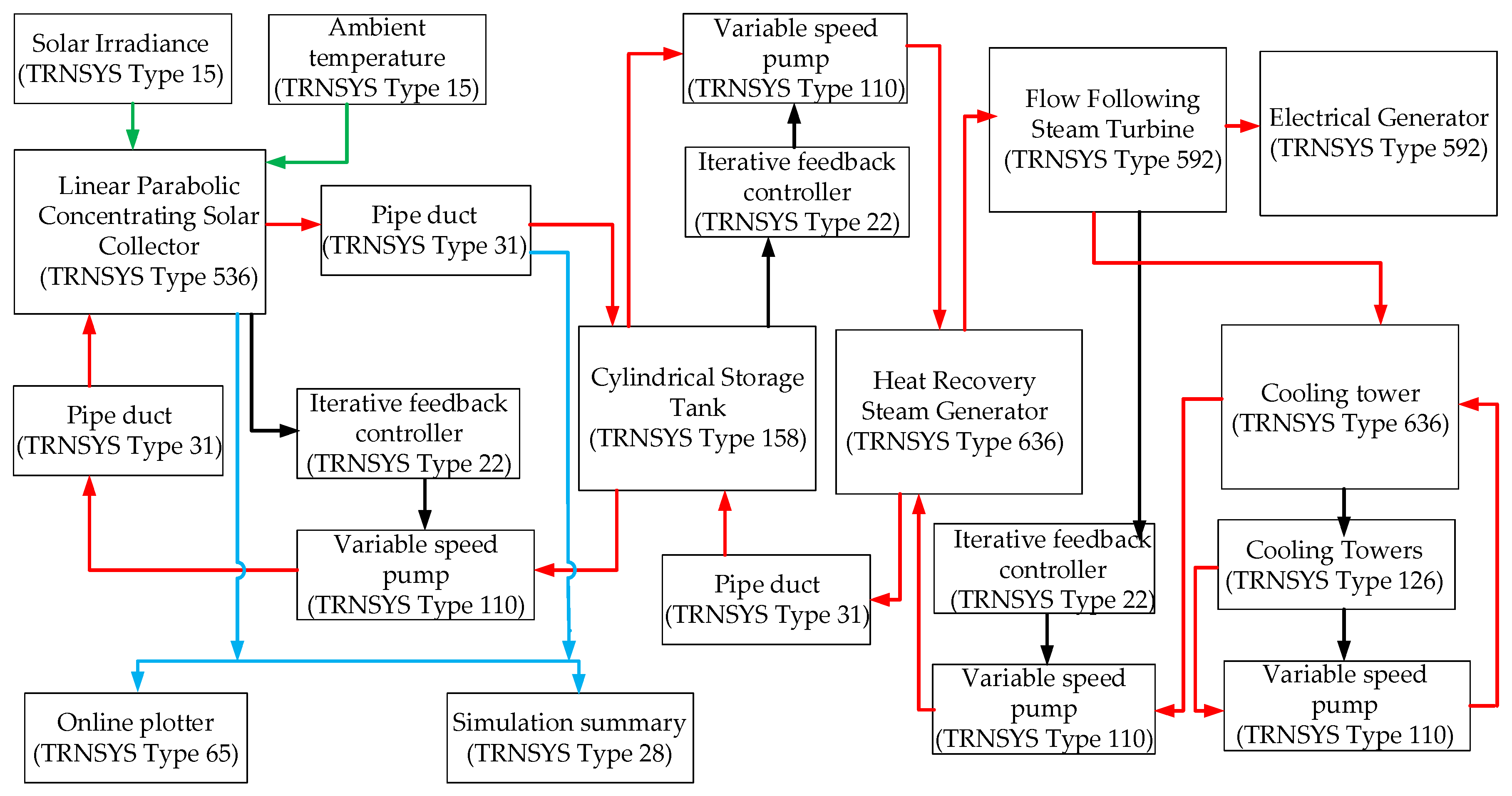
2.2. PCS Model
3. Testing of the Solar Thermal Power Generation Plant
3.1. Distributed Collector System
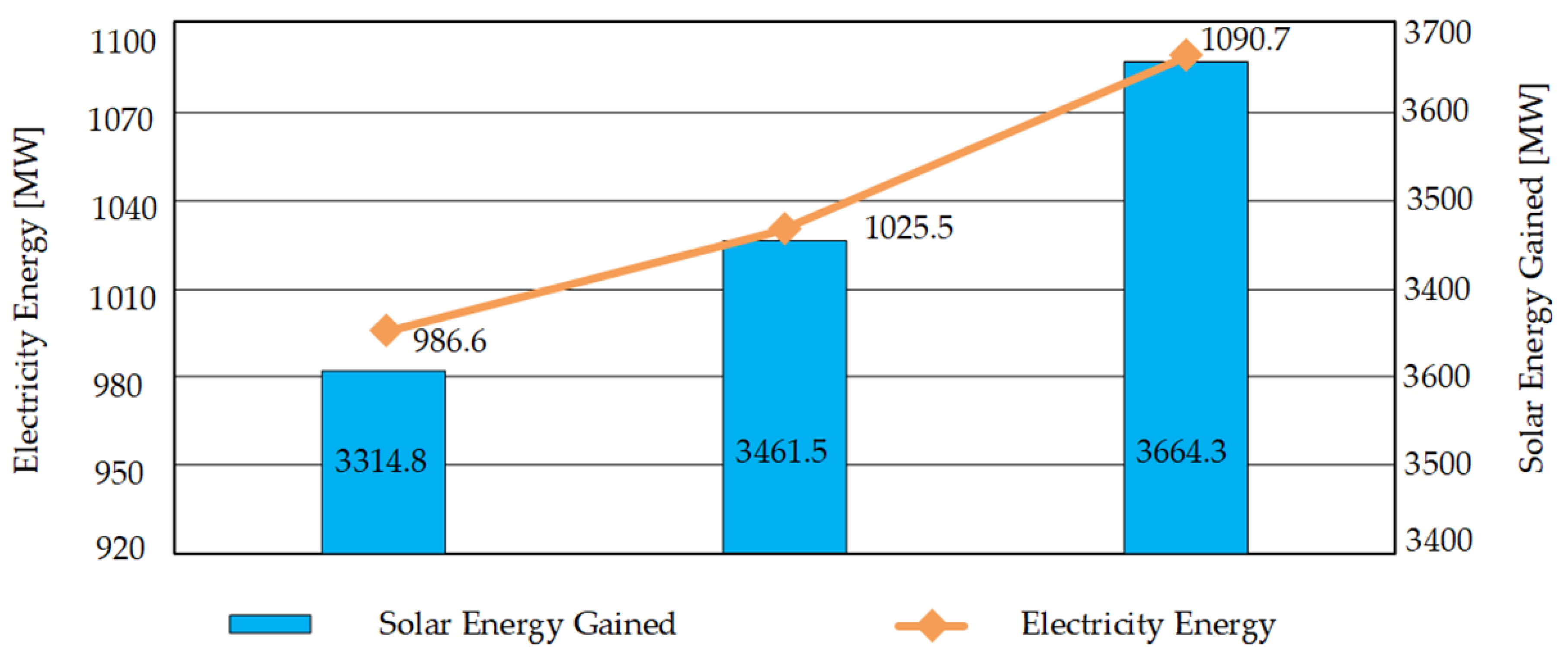
3.2. Performance of the Plant
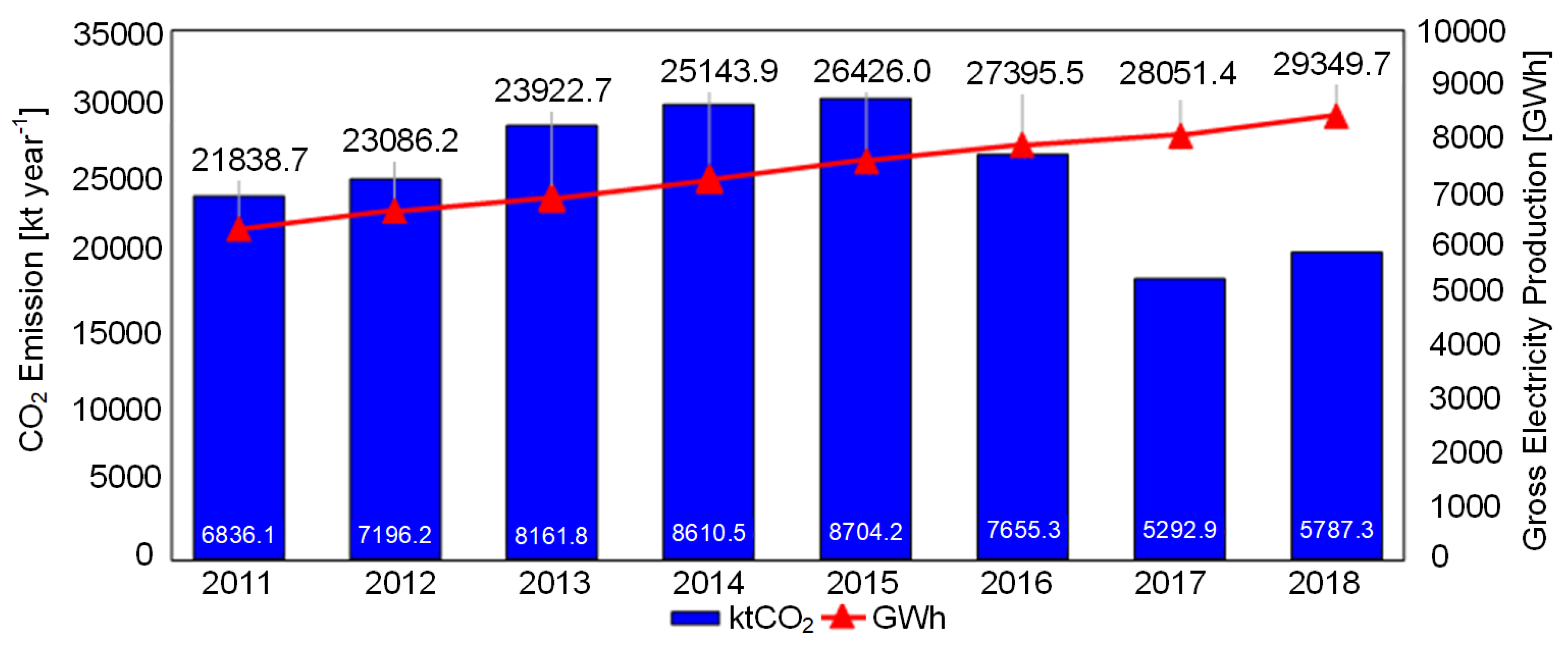
4. CO2 Emissions
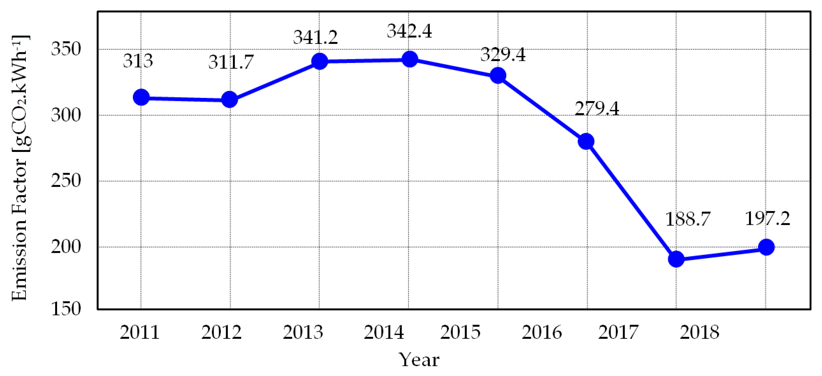
4.1. Emission Factor
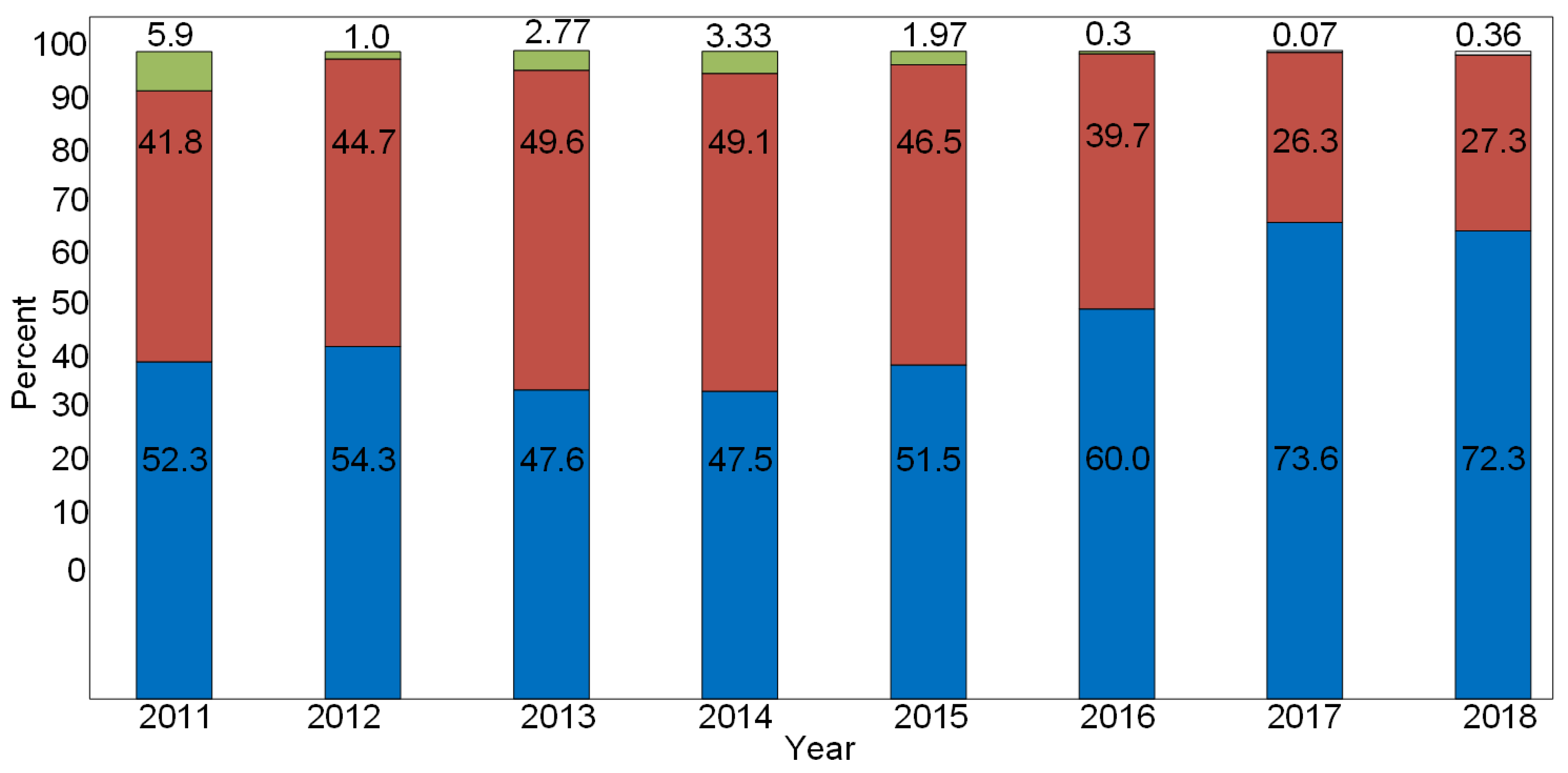
4.2. Results and Discussion of Emission Factors
5. Conclusions
Author Contributions
Funding
Conflicts of Interest
Nomenclatue
| Symbol | Description Unit | ||
| Collector absorber cross-sectional area () | |||
| Specific heat capacity () | |||
| Conversion factor to account for the number of modules, connections, and conversion () | |||
| Outlet fluid temperature-inlet fluid temperature-related transport delay in | |||
| Output signal function | |||
| Quantity of fossil fuel type i consumed in the year y of the generation units m ( | |||
| Energy density by weight of fossil fuel type i in the year y () | |||
| CO2 emission factor of the generation units m in the year y () | |||
| CO2 emission factor by fuel type i in the year y () | |||
| Net energy generated in the year and except for low-cost units () | |||
| Collector aperture () | |||
| Thermal losses coefficient ) | |||
| Linear function of thermal losses () | |||
| Fuels used by generation units m in the | |||
| Year solar irradiance | |||
| k | Generation units connected to the grid in the year y | ||
| Optical efficiency | |||
| Loop pipe length () | |||
| Equivalent length of the collector (m) | |||
| Primary circuit mass flow rate () | |||
| Geometric efficiency (Unitless) | |||
| Number of operational loops (Unitless) | |||
| Number of parallel collectors in each loop-row (Unitless) | |||
| Number of serial tubes in each collector (Unitless) | |||
| Volumetric flow rate in the loop | |||
| Volumetric flow rate in Power Conversion System | |||
| Volumetric flow rate in solar field collector | |||
| Ambient temperature (°C) | |||
| Mean fluid temperature (°C) | |||
| Inlet temperature of the loop (°C) | |||
| Outlet temperature of the loop (°C) | |||
| Inlet temperature in the Power Conversion System (°C) | |||
| Outlet temperature in the Power Conversion System (°C) | |||
| Inlet temperature of the solar field collector (°C) | |||
| Outlet temperature of the solar field collector (°C) | |||
| Flow rate (m·s−1) | |||
| Tracking error | |||
| Controlled variable | |||
| Set-point | |||
| Greek symbol | |||
| Increased enthalpy (J·kg−1) | |||
| Water density (kg·m−3) | |||
| LPG | Liquefied Petroleum Gas (l) | ||
| Density | Energy Density by Weight | ||
| Value | Unit | Value | Unit |
| 944.0 | kg·m−3 | 11.2 | kWh·kg−1 |
| 850.0 | kg·m−3 | 11.6 | kWh·kg−1 |
| 739.0 | kg·m−3 | 12.4 | kWh·kg−1 |
| 0.67 | kg·m−3 | 10.7 | kWh·kg−1 |
| 944.0 | kg·m−3 | 2.2 | kWh·kg−1 |
| 874.0 | kg·m−3 | 11.6 | kWh·kg−1 |
| 528.6 | kg·m−3 | 13.7 | kWh·kg−1 |
| 120.0 | kg·m−3 | 4.76 | kWh·kg−1 |
| 1.15 | kg·m−3 | 1.48 | kWh·kg−1 |
References
- Rasiah, R.; Al-Amin, A.Q.; Ahmed, A.; Leal, W.; Calvo, E. Climate mitigation roadmap: Assessing low carbon scenarios for Malaysia. J. Clean. Prod. 2016, 133, 272–283. [Google Scholar] [CrossRef]
- Mcinerney, C.; Johannsdottir, L. Lima Paris Action Agenda: Focus on Private Finance—Note from COP21. J. Clean. Prod. 2016, 126, 707–710. [Google Scholar] [CrossRef]
- Krismadinata, N.; Abd, N.R.; Ping, H.W.; Selvaraj, J. Photovoltaic module modelling using Simulink/MatLab. Procedia Environ. Sci. 2013, 17, 537–546. [Google Scholar] [CrossRef] [Green Version]
- Camacho, E.; Berenguel, M.; Rubio, F.; Martinez, D. Control of Solar Energy Systems; Springer: Berlin/Heidelberg, Germany, 2012. [Google Scholar]
- Alsharkawi, A.; Rossiter, J.A. Distributed Collector System: Modelling, Control, and Optimal Performance Keywords. Autom. Control Parabol. Solar Therm. Power Plant 2015, 13, 1–6. [Google Scholar] [CrossRef]
- Perers, B.; Furbo, S. IEA-SHC Tech Sheet 45.A.4 Simulation of Large Collector Fields [WWW document]. 2018. Available online: http://task45.iea-shc.org/fact-sheets (accessed on 23 March 2019).
- Barcia, L.A.; Peón Menéndez, R.; Martínez Esteban, J.Á.; José Prieto, M.A.; Martín Ramos, J.A.; De Cos Juez, F.J.; Nevado Reviriego, A. Dynamic Modeling of the Solar Field in Parabolic Trough Solar Power Plants. Energies 2015, 8, 13361–13377. [Google Scholar] [CrossRef] [Green Version]
- Barcia, L.A.; Peon, R.; Díaz, J.; Pernía, A.M.; Martínez, J.Á. Heat Transfer Fluid Temperature Control in a Thermoelectric Solar Power Plant. Energies 2017, 10, 1078. [Google Scholar] [CrossRef] [Green Version]
- Michael, J.; Wolfgang, G.; Mollenbruck, F.; Monnigmann, M. Plant-wide control of a parabolic trough power plant with thermal energy storage. In The International Federation of Automatic Control; National Member Organizations: Cape Town, South Africa, 2014; pp. 419–425. [Google Scholar]
- Dinter, F.; Möller, L. A review of Andasol 3 and perspective for parabolic trough CSP plants in South Africa. In AIP Conference Proceedings; AIP Publishing LLC: Melville, NY, USA, 2016; Volume 1734. [Google Scholar]
- Khenissi, A.; Krüger, D.; Hirsch, T.; Hennecke, K. Return of experience on transient behavior at the DSG solar thermal power plant in Kanchanaburi, Thailand. Energy Procedia 2015, 69, 1603–1612. [Google Scholar] [CrossRef] [Green Version]
- Jebasingh, V.K.; Herbert, G.M.J. A review of solar parabolic trough collector. Renew. Sustain. Energy Rev. 2016, 54, 1085–1091. [Google Scholar] [CrossRef]
- Llamas, J.M.; Bullejos, D.; de Adana, M.R. Optimal operation strategies into deregulated markets for 50 MWe parabolic trough solar thermal power plants with thermal storage. Energies 2019, 12, 935. [Google Scholar] [CrossRef] [Green Version]
- Linrui, M.; Zhifeng, W.; Dongqiang, L.; Li, X. Establishment, validation, and application of a comprehensive thermal-hydraulic model for a parabolic trough solar field. Energies 2019, 12, 1–24. [Google Scholar]
- Camacho, E.F.; Gallego, A.J. Optimal operation in solar trough plants: A case study. Sol. Energy 2013, 95, 106–117. [Google Scholar] [CrossRef]
- Bava, F.; Furbo, S. Development and validation of a detailed TRNSYS-MATLAB model for large solar collector fields for district heating applications. Energy 2017, 135, 698–708. [Google Scholar] [CrossRef] [Green Version]
- Drosou, V.; Valenzuela, L.; Dimoudi, A. A new TRNSYS component for parabolic trough collector simulation. Int. J. Sustain. Energy 2016, 209–229. [Google Scholar] [CrossRef]
- Jansuya, P.; Kumsuwan, Y. Design of MATLAB/Simulink Modeling of Fixed-Pitch Angle Wind Turbine Simulator. Energy Procedia 2013, 34, 362–370. [Google Scholar] [CrossRef] [Green Version]
- Xiufan, L.; Yiguo, L. Transient analysis and execution-level power tracking control of the concentrating solar thermal power plant. Energies 2019, 12, 1–17. [Google Scholar]
- Erdenedavaa, P.; Rosato, A.; Adiyabat, A.; Akisawa, A.; Id, S.S.; Ciervo, A. Model analysis of solar thermal system with the effect of dust deposition on the collectors. Energies 2018, 11, 1795. [Google Scholar] [CrossRef] [Green Version]
- Li, C.; Wang, N.; Zhang, H.; Liu, Q.; Chai, Y.; Shen, X.; Yang, Z.; Yang, Y. Environmental Impact Evaluation of Distributed Renewable Energy System Based on Life Cycle Assessment and Fuzzy Rough Sets. Energies 2019, 12, 4214. [Google Scholar] [CrossRef] [Green Version]
- Ampuño, G.; Roca, L.; Berenguel, M.; Gil, J.D.; Pérez, M.; Normey-Rico, J.E. Modeling and simulation of a solar field based on flat-plate collectors. Solar Energy 2018, 170, 369–378. [Google Scholar] [CrossRef]
- Gíuliano, S.; Buck, R. Analysis of Solar-Thermal Power Plants with Thermal Energy Storage and Solar-Hybrid Operation Strategy. J. Energy Eng. 2011, 133, 1–8. [Google Scholar] [CrossRef]
- Aidroos, D.; Abdul, H.; Zaidi, W.; Omar, W. Historical development of concentrating solar power technologies to generate clean electricity efficiently—A review. Renew. Sustain. Energy Rev. 2015, 41, 996–1027. [Google Scholar]
- Guney, M.S. Solar power and application methods. Renew. Sustain. Energy Rev. 2016, 57, 776–785. [Google Scholar] [CrossRef]
- Khan, J.; Arsalan, M.H. Solar power technologies for sustainable electricity generation—A review. Renew. Sustain. Energy Rev. 2016, 55, 414–425. [Google Scholar] [CrossRef]
- Carmona, R. Análisis Modelado y Control de un Campo de Colectores Solares Distribuidos con un Sistema de Seguimiento de un eje. Ph.D. Thesis, Universidad de Sevilla, Sevilla, Spain, 1985. [Google Scholar]
- Camacho, E.F.; Berenguel, M.; Gallego, A.J. Control of thermal solar energy plants. J. Process Control 2014, 24, 332–340. [Google Scholar] [CrossRef]
- Alsharkawi, A.; Rossiter, J.A. Dual-Mode MPC for a Concentrated Solar Thermal Power Plant. IFAC-PapersOnLine 2016, 49, 260–265. [Google Scholar] [CrossRef]
- Bayas, A. Diseño de Estrategias de Control Difuso Robusto ante Incertidumbre Paramétrica Para Plantas de Colectores Solares; Universidad de Chile: Ñuñoa, Chile, 2016. [Google Scholar]
- Camacho, E.F.; Berenguel, M. Control of Solar Energy Systems. IFAC Proc. 2012, 45, 848–855. [Google Scholar] [CrossRef] [Green Version]
- Cirre, C.M. Reference governor optimization and control of a distributed solar collector field. Eur. J. Oper. Res. 2009, 193, 709–717. [Google Scholar] [CrossRef]
- TRNSYS 17 a TRaNsient SYstem Simulation program. In Mathematical Reference; Solar Energy Laboratory (Ed.) University of Wisconsin-Madison: Madison, WI, USA, 2010; Volume 5. [Google Scholar]
- Wei, D.; Li, B. Iterative-Feedback-Tuning Control Strategy for Air-conditioning Refrigeration Station Systems. J. Comput. 2017, 28, 335–346. [Google Scholar]
- Agencia de regulación y control de Electricidad (ARCONEL). Estadísticas anual y Multianual del sector eléctrico ecuatoriano 2018; Annual Report for ARCONEL; ARCONEL: Quito, Ecuador, 2018.
- Agencia de regulación y control de Electricidad (ARCONEL). Atlas del Sector Eléctrico Ecuatoriano 2018; Annual Report for ARCONEL; ARCONEL: Quito, Ecuador, 2018.
- Parra, R. Factor de emisión de CO2 debido a la generación de electricidad en el Ecuador durante el periodo 2001–2014. ACI Avances en Ciencias e Ingenierías 2015, 7, 2. [Google Scholar]
- Espín, I.; Ochoa-Herrera, V. Cálculo de las Emisiones de CO2 por Consumo de energía, Consumo de agua y Generación de Residuos en la Universidad San Francisco de Quito Ext; Galápagos y en el Galápagos Science Center; Universidad San Francisco de Quito: Quito, Ecuador, 2015. [Google Scholar]
- Organization for Economic Development and Cooperation. CO2 Emissions from Fuel Combustion 2017, 2017th ed.; Organization for Economic Co-operation & Development: Bonn, Germany, 2017. [Google Scholar]
- Burkhardt, J.; Garvin, H.; Cohen, E. Life Cycle Greenhouse Gas Emissions of Trough and Tower Concentrating Solar Power Electricity Generation Systematic Review and Harmonization. Environ. Sci. Technol. 2012, 16, 93–109. [Google Scholar]
- Burkhardt, J.J.; Heath, G.A.; Turchi, C.S. Life Cycle Assessment of a Parabolic Trough Concentrating Solar Power Plant and the Impacts of Key Design Alternatives. Environ. Sci. Technol. 2011, 45, 2457–2464. [Google Scholar] [CrossRef]
- ISO. Environmental Management Assessment—Life Cycle—Requirements and Guidelines; ISO: Genève, Switzerland, 2006; pp. 1–54. [Google Scholar]
- Global Sustainable Electricity Partnership. Proyecto Eólico Isla San Cristóbal—Galápagos; Eólica San Cristóbal S.A.-EOLICSA: Galápagos, Ecuador, 2013. [Google Scholar]


| Property | Quantity |
|---|---|
| Net electrical power | 500 kW |
| Parasites | 77 kW |
| Gross electrical power | 577 kW |
| Gross efficiency | |
| Oil thermal power | |
| Thermal losses | |
| Refrigeration losses |
| Property | Quantity | Unit |
|---|---|---|
| Collector Field | ||
| Collector type | PTC | - |
| Parabolic width | 1.83 | |
| Collector length | 3.05 | |
| No. of collector | 480 | - |
| No. of loop | 10 | - |
| Total mirror area | 2635 | |
| Mirror reflectivity | 0.78 | - |
| Storage Tank | ||
| Type | Cylindrical | |
| Tank volume | 115 | |
| Tank height | 11.2 | |
| Tank loss coefficient | 0.69 | |
| Power Block | ||
| Electric generator output | 0.5 | |
| Turbine capacity | 0.5 | |
| Property | Quantity | Unit |
|---|---|---|
| Steam enthalpy | 25,000 | |
| Steam pressure | 25 | |
| Steam exhaust pressure | 16 | |
| Steam mass flowrate | 36,000 | |
| Steam temperature | 280 | |
| Pinch point temperature difference | 7 |
| Fuel | 2011 | 2012 | 2013 | 2014 | 2015 | 2016 | 2017 | 2018 |
|---|---|---|---|---|---|---|---|---|
| (Units Million) | ||||||||
| Fuel oil (l) | 1208.8 | 1421.6 | 1561.6 | 1676.6 | 1526.6 | 1136.1 | 645.1 | 843.3 |
| Diesel (l) | 783.3 | 60.0 | 804.2 | 843.8 | 965.6 | 842.4 | 491.9 | 519.6 |
| Naphtha (l) | 66.8 | 0.5 | 12.3 | 0.0 | 0.0 | 0.0 | 0.0 | 0.0 |
| Natural gas (m3) | 518.8 | 680.0 | 759.1 | 782.6 | 753.9 | 767.9 | 688.8 | 592.1 |
| Waste (l) | 155.0 | 149.6 | 145.9 | 164.6 | 267.2 | 225.5 | 129.6 | 130.0 |
| Crude (l) | 285.5 | 3055.0 | 343.7 | 350.5 | 341.5 | 456.4 | 461,4 | 508.7 |
| LPG (l) | 32.3 | 28.6 | 26.8 | 28.6 | 33.2 | 37.7 | 32.3 | 35.9 |
| Cane bagasse (t) | 1064.3 | 1122.3 | 343.5 | 1447.7 | 1504.4 | 1542.8 | 1668.5 | 1437.1 |
| Biogas (m3) | 0 | 0 | 0 | 0 | 0 | 8,119,299.9 | 16,327,344.0 | 26,622,714.2 |
| Fuel | 2011 | 2012 | 2013 | 2014 | 2015 | 2016 | 2017 | 2018 |
|---|---|---|---|---|---|---|---|---|
| Fuel oil | 2970.9 | 3493.5 | 3838.0 | 4120.5 | 3751.4 | 2792.8 | 1583 | 2072.8 |
| Diesel | 1755.2 | 1417.8 | 1802.3 | 1890.7 | 2163.7 | 1887.7 | 1102.7 | 1164.5 |
| Naphtha | 134.6 | 0.8 | 24.7 | 0 | 0 | 0 | 0 | 0 |
| Natural gas | 907.7 | 1190.6 | 1327.5 | 1365.9 | 1318.3 | 1341.9 | 1206 | 1035.9 |
| Waste | 381.5 | 367.2 | 358.8 | 405.1 | 656.9 | 554.2 | 318.1 | 319.7 |
| Crude | 644.3 | 688.9 | 775.5 | 790.8 | 770.6 | 1029.6 | 1041.1 | 1147.6 |
| Liquefied gas Petroleum | 41.9 | 37.3 | 35.0 | 37.6 | 43.2 | 49.2 | 42.1 | 46.9 |
| * Cane bagasse | 827.4 | 872.5 | 850.0 | 1124.9 | 1169.6 | 1199.4 | 1297.1 | 1117.2 |
| * Biogas | 0 | 0 | 0 | 0 | 0 | 8897.1 | 29,173 | |
| Total | 6836.1 | 7196.1 | 8161.8 | 8610.5 | 8704.2 | 7655.3 | 5292.9 | 5787.3 |
| Life Cycle Phase | Plant System | GHG (g CO2eq·kWh−1) |
|---|---|---|
| Manufacturing | HTF Power plant Solar field TES | 13 |
| Construction | 1.8 | |
| Operation | 11 | |
| Dismantling | 0.12 | |
| Disposal | 2.1 | |
| Grand total | 26 |
| Selected Sites | Electricity Energy MWh | Gallons Saved | Invoicing Dollars | Emissions TON CO2 Generated by the Thermo-Solar Plant | Emissions TON CO2 Avoided When Not Using Fuel | Total Emissions TON CO2 Avoided |
|---|---|---|---|---|---|---|
| Guayaquil | 411.1 | 35,747.8 | 52,703.0 | 10.7 | 81.0 | 70.3 |
| Manta | 497.2 | 43,234.8 | 63,741.0 | 12.9 | 98.0 | 85.1 |
| San Cristóbal | 680.6 | 59,182.6 | 87,252.9 | 17.7 | 544.4 | 526.7 |
© 2020 by the authors. Licensee MDPI, Basel, Switzerland. This article is an open access article distributed under the terms and conditions of the Creative Commons Attribution (CC BY) license (http://creativecommons.org/licenses/by/4.0/).
Share and Cite
Ampuño, G.; Lata-Garcia, J.; Jurado, F. Evaluation of Energy Efficiency and the Reduction of Atmospheric Emissions by Generating Electricity from a Solar Thermal Power Generation Plant. Energies 2020, 13, 645. https://doi.org/10.3390/en13030645
Ampuño G, Lata-Garcia J, Jurado F. Evaluation of Energy Efficiency and the Reduction of Atmospheric Emissions by Generating Electricity from a Solar Thermal Power Generation Plant. Energies. 2020; 13(3):645. https://doi.org/10.3390/en13030645
Chicago/Turabian StyleAmpuño, Gary, Juan Lata-Garcia, and Francisco Jurado. 2020. "Evaluation of Energy Efficiency and the Reduction of Atmospheric Emissions by Generating Electricity from a Solar Thermal Power Generation Plant" Energies 13, no. 3: 645. https://doi.org/10.3390/en13030645