Empirical Models for the Estimation of Solar Sky-Diffuse Radiation. A Review and Experimental Analysis


1
Department of Mechanical Engineering, University of the Basque Country, 01006 Vitoria-Gasteiz, Spain
2
School of Civil Engineering, University of Granada, 18071 Granada, Spain
3
School of Engineering and the Built Environment, Edinburgh Napier University, Edinburgh EH10 5DT, UK
*
Author to whom correspondence should be addressed.
Energies 2020, 13(3), 701; https://doi.org/10.3390/en13030701
Submission received: 13 October 2019
/
Revised: 2 February 2020
/
Accepted: 3 February 2020
/
Published: 6 February 2020
(This article belongs to the Special Issue Recent Advances in Sustainable Buildings: Space Heating, Space Cooling and Lighting)
Abstract
:Accurate solar radiation data are essential for the development of solar energy application systems. The limited availability of solar radiation data, and especially diffuse irradiance values, makes it vital to develop models to estimate these data. The development of estimation models has been the objective of many studies. This paper presents an extended review of the diffuse ratio (k) vs. clearness index (kt) annual, monthly, daily, and hourly frequency regression models. It is however interesting to note that there is a dearth of such knowledge for diffuse ratio–clearness index regressions that are based on averaged data. Monthly-averaged daily global irradiation data are now easily available from the NASA website for any global location. Using existing models, it is possible to decompose the daily to averaged-hourly global irradiation values. The missing link so far has been hourly averaged diffuse irradiation. This article presents regression equations which could be used to estimate that information. For this purpose, hourly global and diffuse irradiation data was pooled from 19 different locations to obtain three latitude-dependent regression models relating the monthly-averaged hourly diffuse ratio () to the clearness index (). The results show a high relationship between both variables. These regression equations could be used to estimate the averaged diffuse irradiation values from averaged global irradiation values, which are more easily available.
1. Introduction
Alternative or renewable energy sources are able to provide the global current and future energy, with zero or almost zero greenhouse gas and pollutant emissions [1]. The sun is the most significant source of renewable energy available; it is not only naturally replenished, clean, and environmentally friendly, but it also drives the bases of the earth and causes nearly all the energy sources known today. Wind and hydro energy, biomass, and even fossil fuels are available because of the sun. Solar energy can generate heat and electricity for domestic and industrial use, and research in the field has increased significantly the efficiency and capacity of solar energy technologies. However, the potential of solar applications is much higher than the present use of this energy source.
The amount of energy generated from solar energy depends directly on the quantity of solar irradiance that is received in the earth and the efficiency of the devices used in the conversion process [2]. For a proper evolution of solar energy application systems, it is indispensable to have solar radiation data. Solar water heating, photovoltaic and solar-driven ventilation systems, daylighting and building air conditioning are some solar energy applications where solar irradiance figures are required to obtain solar energy resource assessment. However, most of the meteorological stations only have records of global irradiation data measured on the horizontal plane. Weather stations rarely register direct and diffuse solar fractions [3].
The most demanded radiation data are mainly global and diffuse horizontal irradiation in hourly or sub-hourly frequency. However, it is not always possible to get long-term series for the previously mentioned parameters. Even though global irradiation at a monthly, daily, or hourly basis is the most commonly recorded parameter, it is only available in a limited number of meteorological stations. For example, there are 71 and 31 stations that measure these parameters in the UK and Spain, respectively.
It is much more expensive and relatively more complicated to measure the diffuse and direct components, and in consequence, these irradiation records are even scarcer than the global irradiation measurements [4]. In the UK for example, since 2002, the diffuse irradiation is measured in just two locations, at Lerwick (60.80° N) and Northern Camborne (55.21° N).
There are more meteorological stations that measure daily rather than hourly irradiation values, and it is more common to have daily global values rather than global and diffuse values. Almost all the radiometric stations are equipped with pyrarometers to measure global solar irradiance, but only a few stations have equipment to measure the diffuse component of the solar tilted [5].
However, the contribution of the diffuse sky component in the irradiance received in the earth’s surface is high enough to consider the diffuse irradiation an essential parameter for projects related to solar energy.
In South Africa, where much of the country is in the rather cloud-free anticyclonic belt of Southern Hemisphere, the diffuse irradiation contributes about the 30% of the annual short-wave energy received. In most of locations of this country, 523,000 and 581,111 Wh/m2 are received indirectly over a year. This value is similar to 546,244 and 499,756 Wh/m2 that Brussels and Berlin receive respectively during a year, where the ratio between diffuse and total irradiation is 0.55. In Antananarivo (Madagascar), the diffuse irradiation contributes the 40% (813,556 Wh/m2) of the annual total irradiation [6].
The diffuse irradiance is significant in many fields. One of those fields is the heat transfer application in buildings, where the irradiation is particularly important in tropical and sub-tropical climates where the energy contribution can reach very high levels. In the use of the solar energy, for example in the supply of hot water for domestic use, the diffuse irradiance can determine the continued efficiency of the process [6]. For house energy analysis, diffuse irradiance data are also required [7].
In those situations, it is essential to create correlation models to estimate diffuse irradiation data from the global irradiation records.
Therefore, numerous researchers have established empirical links to predict sky-diffuse irradiation based on available input variables, the clearness index (kt) being one of the most important ones [4,8,9]. The clearness index relates the global and the extraterrestrial irradiation.
Liu and Jordan [10] were pioneers on the study of the correlation between diffuse ratio (k) and clearness index (kt). Since then, several research teams have produced regression equations relating the previously mentioned parameters at an annual, monthly, daily, and hourly frequency for locations all over the world. Each regression equation is unique and statistically different.
The limited availability of solar radiation data records makes it essential to estimate irradiation values for sloped surfaces given values for horizontal surface. As mentioned before, the available radiation records are commonly for global irradiation on a horizontal surface. However, very few applications use the horizontal configuration; solar collectors for example are mounted tilted at some angle to it. Solar radiance data on tilted surfaces are essential prerequisites in several sciences. Agricultural meteorology, photobiology, animal husbandry, daylighting, and solar energy utilization, among others, require information about the available solar irradiance on slopes. The solar irradiance on a horizontal surface differs from the irradiance on a tilted surface [11].
Thus, this is an added reason for estimating diffuse irradiation values using correlation models [7], since both beam and diffuse irradiation components are used to estimate slope irradiance. It is not possible to merely estimate the irradiation using trigonometric relationships, since the diffuse irradiance is not isotropic over the sky dome [12]. The irradiance that gets to the inclined collector does not only depend on its orientation but it is also affected by the assumed distribution that the diffuse irradiance has across the sky [7]. Once direct and diffuse irradiation values are estimated using correlation models, they can then be transported over tilted surfaces. This way, it is possible to estimate the completion of tilted flat plane collectors and other solar devises [13].
The estimation models’ uncertainty and credibility will directly depend on the uncertainty of the available radiation data of any location. The more detailed the records are, the more accurate the predictions will be [11].
Considering the limited availability of the diffuse irradiation measurements and its importance in solar energy applications, the objectives of this article are:
- Monthly-averaged daily global radiation data are now easily available from NASA website for any global location. Using existing models, it is then possible to decompose the daily to averaged-hourly global irradiation. The missing link so far has been hourly averaged diffuse irradiation. This article intends to provide regression models to estimate the average-hourly diffuse irradiation using the freely accessible NASA website data.
2. Annual Average Diffuse Irradiation
Agricultural use of solar energy requires monthly or even annual irradiation data. The diffuse irradiation records are very scarce, and correlation models need to be established to estimate the diffuse component from the available parameters [14].
A great number of researchers have investigated the relationship between the annual k and the corresponding kt. Muneer [11] developed the Equation (1) using data from several Indian meteorological stations (Gilat, Qrendi, Khormaskar, Tashkent, and Nice), which shows a strong correlation between both variables.
Muneer and Hawas [15] analyzed data from 13 stations in India and showed that the annual global to extraterrestrial radiation fraction (kt annual) varies between 0.53 and 0.61 in the tropics. The ratio of annual values of diffuse to extraterrestrial radiation (kt annual) varies in a very narrow range, between 0.22 and 0.25 with an average value of 0.233. Stanhill [16] used three years of radiation values records in the south of Israel to develop a correlation between the annual diffuse to extraterrestrial ratio, and compared these relationships with those obtained in other locations to verify their applicability in the region. The ratio between the annual diffuse and extraterrestrial radiation reported by Stanhill for Gilat is 0.237. This value is also comparable to the results obtained for several UK locations, where the average value of the annual ratio was again 0.233 [11]. Other researchers, such as Mani and Chacko and Drummond, obtained diffuse to extraterrestrial values of 0.36 and 0.3, respectively [11].
According to Muneer it is easily possible to compute the annual–average extraterrestrial irradiation. Therefore, using a general value of 0.233 for the ratio between the annual diffuse to extraterrestrial radiation, it would be possible to obtain annual diffuse radiation data for any location [11].
3. Monthly Average Diffuse Irradiation
Specific solar radiation data at any location is needed, especially by solar engineers and architects [14]. The annual diffuse irradiation data are not enough for various solar energy applications, such as concentrating collectors, solar furnaces, etc. At least monthly diffuse irradiation data are needed for these applications. Therefore, for the locations where only the horizontal global irradiation is recorded, models to estimate diffuse irradiation are needed [17].
The monthly-average daily diffuse irradiation has been calculated considering the monthly average daily kt as an independent variable (Equation (2)) [18].
Many experimental regression equations to estimate the monthly-averaged daily diffuse irradiation have been presented during the last decades [13]. The first correlation model between the monthly-averaged values of diffuse and global irradiation was defined by Liu and Jordan [10]. This model, together with the one brought by Page, are two of the most popular correlations [19]. From this pioneer research, a high number of regression models have been developed by fitting datasets from different places and frequencies [4]. Iqbal presented a correlation model between the k (Hd/H) and the fraction of the number of sunshine hours (S/S0) [20]. Gopinathan, on the other hand, presented empirical models relating the k with the kt, fraction of sunshine hours, and a combination of both [21].
Each of those models include experimental constants which are dependent on the time of year and the geographical location, therefore, most models are only valid for a specific place. According to El-Sebaii and Trabea, for example, a correlation between the k and kt is adequate to calculate the month-to month average daily diffuse irradiation in South Africa [7].
4. Daily Average Diffuse Irradiation
In many solar applications, monthly average diffuse irradiation data are not enough. Daily or even hour-by-hour solar irradiation data represent an important requirement. The first regression equation, which relates the daily k and the daily kt, was also developed by Liu and Jordan [10]. This correlation did not consider the shade ring of the kt, and they used just one value of the extraterrestrial irradiation for the middle days of the month.
Choudhary developed a model for New Delhi using only three months of data and obtained higher k values than the Liu and Jordan model [33]. At first, they associated this to the high dust content in New Delhi and the small sample of data. However, as it was proven later, these higher k values are due to the lack of compensation of the shade ring of shadow band in the Liu and Jordan study [11].
Many researchers re-investigated the regression equation presented by Liu and Jordan for different locations in the world and defined new models using daily-integrated data of global and diffuse solar irradiance values. All the investigators calculated the extraterrestrial irradiation for each day. In order to estimate the daily extraterrestrial irradiation, it is possible to use the following equation (Equation (29)) [11].
Collares-Pereira and Rabl used 1‒4 years data for five stations in the USA measured with a pyrheliometer. They confirmed Liu and Jordan’s model’s validity and concluded that the numerical inaccuracies of the original work were due to the use of uncorrected values of diffuse irradiation in the regression, use of a just one value of extraterrestrial insolation during each month, and not taking into account seasonal variations in the diffuse to hemispherical ratio [34]. Even though they found a seasonal trend in the data, they used all data as a group [11]. Table 2 sums up the models correlation daily values of the diffuse irradiation.
Erbs et al. [22] presented two seasonal regression equations, one for winter and another one for the rest of the year. The research was made using mean values of the k over finite intervals of the kt [11], and obtained an equation for each of the seasonal correlations. The equations from the summer data and spring and autumn data were almost equal.
Rao et al. used individual values of k regressed against kt to develop a seasonal as well as an annual regression equation. They developed simple linear regression models and more than 85% in the variability of the fraction between diffuse and global irradiation was explained by the models [35].
Muneer and Hawas [15] used three years of measurements from 13 Indian stations, all of them between 8.5° N and 28.5° N latitude, to develop regression equations for each individual station as well as for the whole country of India. The regression obtained from the equations (Equation (34)) concluded a high relationship between the k and kt for individual locations (R2 = 0.893−0.95) and also for the whole country of India (R2 = 0.89).
Tuller [36] presented a model using one year of daily data from four Canadian stations. They not only found a latitude effect in the results, but also studied the impact the reflectivity of the surface has on the diffuse irradiation, concluding that it only affected in the 27% of the variation for the diffuse transmission coefficient [11].
Saluja and Muneer [37] studied three years of data from five locations in the UK (Easthhampstead, Aberporth, Aldergrove, Eskdalemuir, and Lerwick) and presented a single regression equation for each station and a single correlation model for the five locations.
5. Instantaneous Hourly Diffuse Irradiation
Monthly irradiation data and even daily irradiation data are not enough for many solar engineering applications systems. For those applications, at least hourly irradiation values are needed. Liu and Jordan [10] were the first researchers investigating the correlation between the diffuse and global radiation on a parallel to the ground surface; however, their original regression model was conceived for daily values instead of hourly values.
Since then, several researchers have developed hourly correlation equations relating the k and the kt.
Orgill and Hollands, using four years of data from Toronto (Canada), presented a liner model to estimate k with the hourly kt. They used a shadow-band pyranometer to measure the diffuse irradiance [38].
Erbs et al., following the work of Orgill and Hollands, developed a regression equation using four locations in the 31–42° N latitude range. They used pyroheliometric data, where the diffuse irradiance was calculated deducing the direct irradiance from the global irradiance, which was recorded with a pyranometer [22].
Reindl et al. developed correlations used data from five locations from Europe and North America in order to minimize the standard error of the models similar to the one presented by Liu and Jordan, analyzing the effect of the most frequently recorded climatic parameters on the diffuse fraction [39].
Hawlader derived the second-order polynomial regression with measurements from a tropical place in Singapur. They suggested an equation to calculate k of the hourly, daily and monthly global insulations on a horizontal surface [40]. The hourly regressions trend was similar to the equations developed by Orgill and Hollands [38] and Spenser [41], supporting the latitude dependence that they claimed.
Chandrasekaran and Kumar developed a fourth-order polynomial regression equation using measurements from a tropical site in Madras (India) [42]. This correlation was compared, using the standard and relative standard deviation, to the ones defined by Orgill and Hollands, Erbs et al. and Reindl et al., which were developed using data from warm locations [22,38,39]. It was shown that the new regression equations are more accurate and the best results were found when the seasonal effect was considered. It was also found that the hour-by-hour k is higher in tropical sites than in warm areas, with a much higher k in the rain season when the hourly kt is higher.
Boland et al. used 15-min data from a meteorological station in Victoria to determine if the smoothing caused with the use of hour-by-hour data has an effect in overall results. They found that it is possible to use the same model for 15-min and hourly data [7].
Miguel et al. developed a third order polynomial regression equation for hourly k values using data from several countries in North Mediterranean locations [43].
Oliveira et al. developed a fourth-order polynomial regression equation with data from a tropical location in Sao Paulo, and determined that the general characteristics of the k regression curves and their seasonal alterations are similar to the ones found by other researchers with similar latitude for hourly, daily, and monthly values [44].
Karatasou et al. presented a third-order polynomial correlations with the objective of reducing the standard error of the regression equations similar to the one developed by Liu and Jordan. The research was based on measurements from Athens, Greece [45]. Using the same records from Athens, Soares et al. presented a fourth-order polynomial equation, including the atmospheric long-wave radiation as an input. It was found that these data improves the neural-network performance [46].
The table below (Table 3) shows a review of the mentioned hourly correlation equation of different researchers. All the models relate the k with kt.
For the estimation of the hourly kt values, it is necessary to estimate the hourly extraterrestrial irradiation values. The following equation can be used for that purpose.
It is important to mention that the long-wave radiation, which provides regional scale cloud-cover information, is more important than more common meteorological variables, such as air temperature and atmospheric pressure.
6. Artificial Neural Networks (ANN)
Artificial intelligence is a promising method to model solar radiation and a few models based on artificial neural network (ANN) have been developed to estimate radiation in different regions of the world. An adaptative neuro-fuzzy approach was defined by Olatomiwa et al. using air temperature and sunshine duration to predict solar radiation in Nigeria [48]. The same researchers also developed a support vector machines firefly algorithm, ANN, and genetic programming models to estimate solar radiation in the Iranian city [49]. Park et al. used a topographic factor and sunshine duration to estimate the spatial distribution of solar irradiance in South Korea [50]. A Markov transitions matrix method was proposed by Aguiar et al. to estimate daily irradiation values kt [51]. A Gaussian model for generating synthetic hourly irradiation was also presented by Aguiar and Collares-Pereira [52]. Amrouche and Pivert used combine spatial modeling and ANN techniques to predict global irradiation in two French locations [53]. Linares-Rodriguez et al. used ANN methods to estimate solar radiation based on latitude, longitude, day of the year, and other climatic parameters in Spain [54].
Furthermore, satellite images are also used to study the solar radiation spatial-temporal variations around the world. Hay was a pioneer in introducing the modeling methods for satellite-based estimates of solar radiation at the Earth’s surface [55]. Cano et al. developed a method to estimate the global irradiation form meteorological satellite data [56]. Antonanzas-Torres et al. compared the global solar irradiation values from a satellite estimate model and on-ground measurement in Spain [57].
However, most of the presented models to estimate solar radiation are based on parameters that are more readily available. Some of these parameters are extraterrestrial irradiation, mean temperature, maximum temperature, soil temperature, relative humidity, number of rainy days, altitude, latitude, total precipitation, cloudiness, and evaporation, among others [58].
7. Monthly Average Hourly Diffuse Irradiation: Experimental Analysis
In the NASA website (http://eosweb.larc.nasa.gov) it is currently available information to get daily-averaged irradiation data for most of the worldwide locations. This information includes long-term estimated values of meteorological measures and surface solar energy fluxes provided by satellite systems. These data meet the needs of renewable energy community and it has been proven they are accurate enough to provide consistent solar and meteorological data for locations where records are scarce or non-existent [59].
The information that is provided in the NASA website, which is available in the public domain, can be used to construct a computational chain to get all means of solar energy estimations that need hour-by-hour horizontal and slope, global, and diffuse irradiation data.
7.1. Step 1. Monthly-Averaged Hourly Global Irradiation
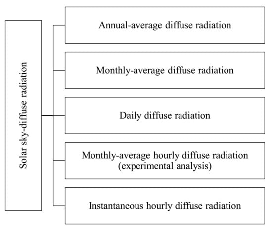
The first step to estimate all manners of solar energy data is to decompose the freely obtainable monthly-averaged daily irradiation data from the NASA website into monthly-averaged hour-by-hour global irradiation values (Figure 1).
Hourly irradiation data requires a very accurate modelling of solar processes. Therefore, the hourly average irradiation is the nearest approach to the real average radiation, which is obtainable from the commonly available solar radiation data [11].
Daily solar irradiation records are more accessible since more locations have the technology to measure it. It is logical to consider that there exists a correlation between daily and hourly solar irradiation.
Whillier was a pioneer in this field. They plotted experimental ratios between daily to hourly global solar irradiation data derived from widely separated locations against the sunset hour angle [62].
A mean curve was obtained for every hour, and it was proved that the deviation of any single point from the mean curve was not higher than ±5% for the hours between 9 am and 3 pm sun time.
Meteorological stations usually publish monthly-averaged values of daily global irradiation. However, when this information is not available, it could be obtained from solar models which use the long-term sunshine data [11].
Liu and Jordan developed a set of correlation curves extending Willier’s work, which shows the effect of the day length and the shift of the hour form solar noon on the ration between the hourly to daily irradiation [10]. These regression curves enable the calculation of the averaged-hourly irradiation data when daily irradiation records are available.
7.2. Step 2. Experimental Analysis
For the experimental analysis of this study, nineteen worldwide locations were chosen, with available hour-by-hour global and diffuse irradiation values in the period (1990 to 2002) found in the respective meteorological office for each location. The table below (Table 4) shows the latitude and longitude and period of observation of each location.
Monthly-averaged hourly values were estimated for the global and diffuse irradiation using the information of each location for the given period of time. A visual basic code was then defined for this purpose. The monthly average hourly diffuse ratio () and the clearness index () were calculated for each location. In order to avoid erroneously recorded data, the conditions below (Equations (49) and (50)) were used. Extraterrestrial irradiation cannot be greater than global irradiation and diffuse irradiation cannot be greater than global irradiation.
Radiance, expressed as W/m2 is the emanating power from a radiating source, on the other hand irradiance is the receipt of radiated power at the receiving surface. Radiation and irradiation, likewise are energy quantities that are expressed as Wh/m2 or kWh/m2. The latter is the integration of power over a given interval of time, so one may have the power integrated over a five-minute or an hour time interval. The UK meteorological office has one of the oldest solar radiation recording networks in the world and their radiation records are available as hourly-integrated values expressed as Wh/m2 [11].
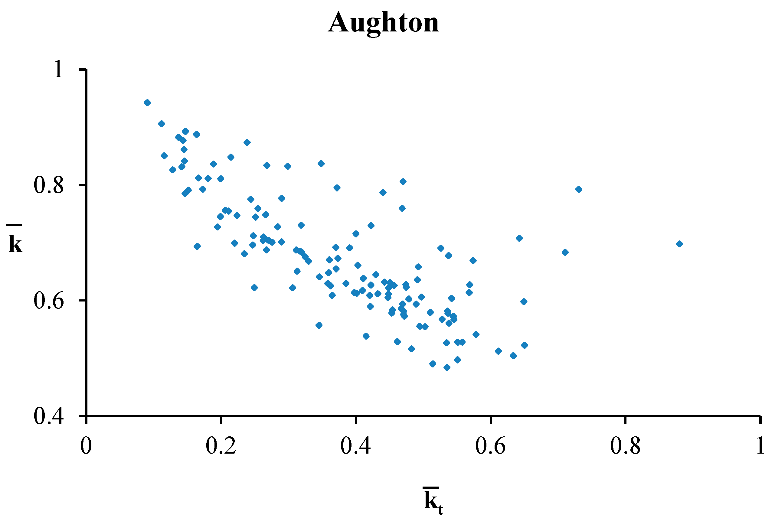
The monthly-averaged kt of the 19 locations was regressed against the monthly-averaged k. The following figures (Figure 2, Figure 3 and Figure 4) show the corresponding scatter plot.
In addition, for a 0.05 width increment of the bandwidth of the kt, the respective values of averaged k were obtained. The table below (Table 5) shows the average k and the average kt in the columns one and two, respectively. The third column presents the number of points considered to calculate the average values. The values in italics correspond to average values calculated only with one or two points. These average values have not been taken into account, since there is not enough information to assure those data are reliable.
The following figures (Figure 5, Figure 6 and Figure 7) show the averaged k and kt plots for each location.
The same process was repeated with all the locations. Figure 8 shows the regression of the average values of k and kt of the 19 worldwide locations together.
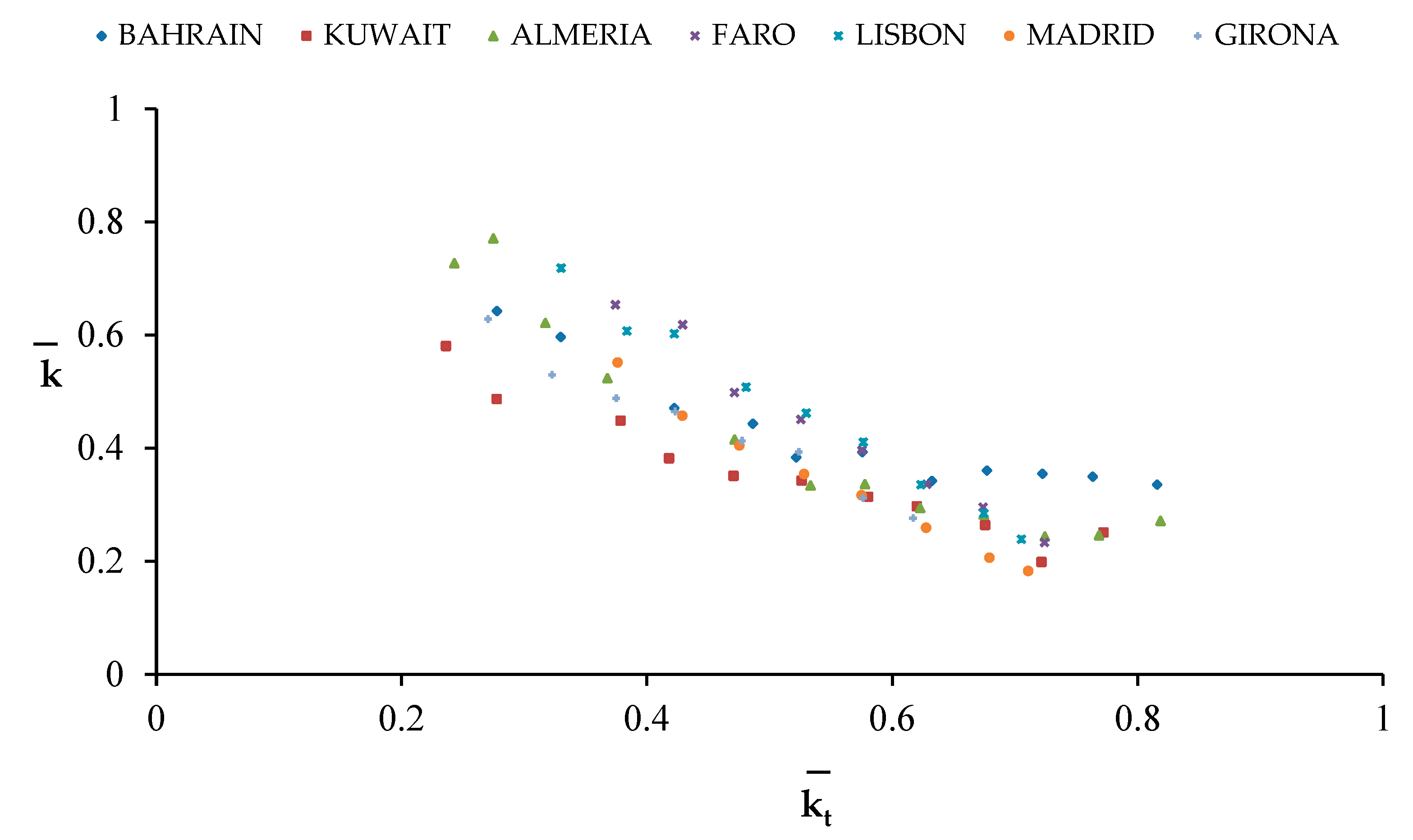
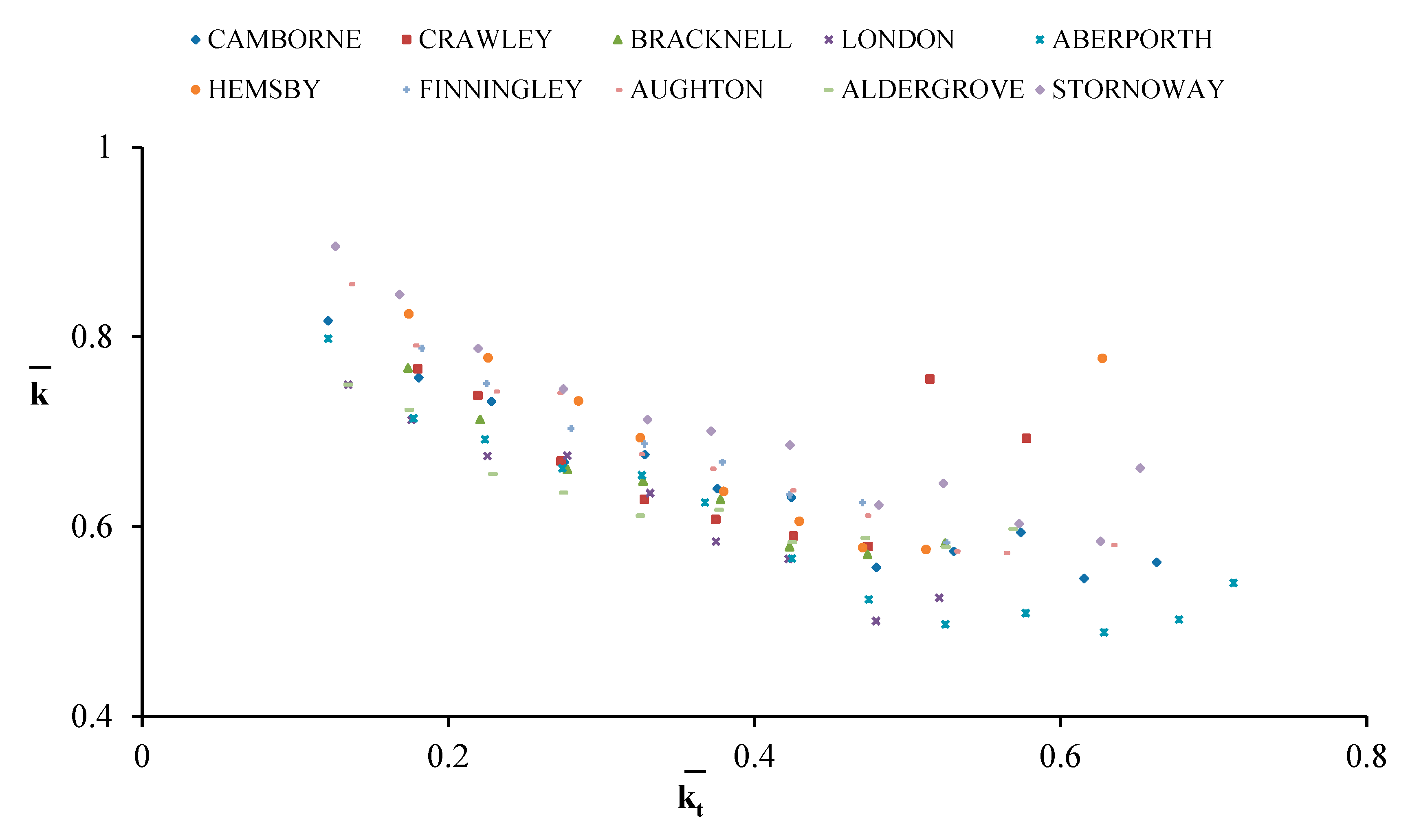
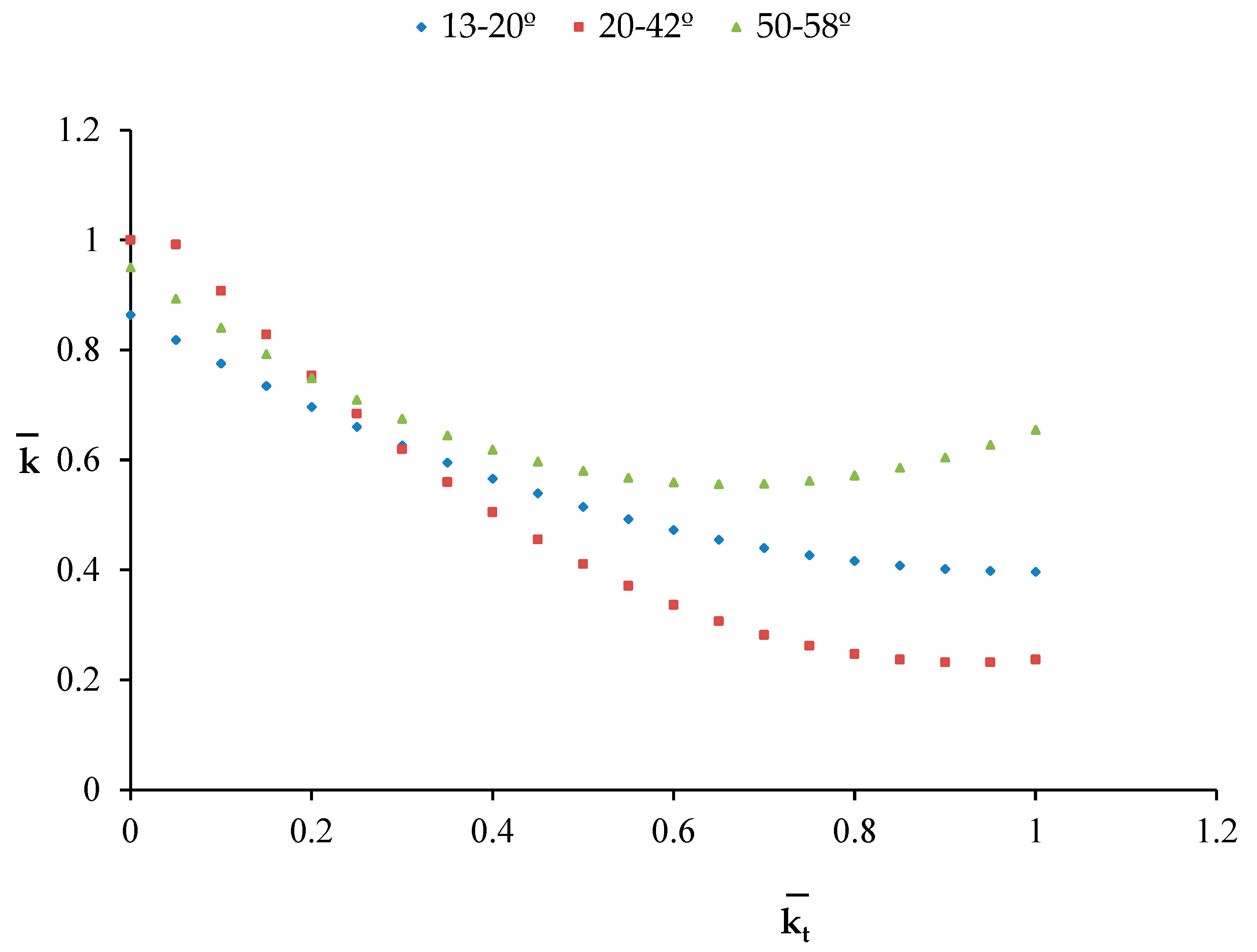
Even though it is not possible to obtain a unique regression equation for the 19 locations, due to the high dispersion of the results, the graph clearly indicates the existence of different sub-models. Therefore, the data have been settled in an increasing order of latitude. Figure 9, Figure 10 and Figure 11, respectively show the regression curves for the locations in a narrower range of latitude.
The three figures (Figure 9, Figure 10 and Figure 11) show the potential for a single regression model for each latitude group.
There is an increasing tendency of k in the top end of kt. This fact is especially notorious in the data from the 10 locations of the highest latitude group that are under examination, as can be seen in Figure 10. This phenomenon is related with simultaneous existence of two astronomical/weather-related situations. A more extended explanation of this phenomenon is developed in Muneer et al. [50].
The Figure 12 shows the definitive regression curves for the three latitude ranges.
The definitive regression equations to estimate monthly-averaged hourly diffuse irradiation values for the latitude ranges developed are shown in the Table 6 below:
There are three main points worth mentioning in this study. First, it is not possible to obtain a unique regression equation for the nineteen worldwide locations. However, a high correlation is observed between the average k and kt, with high values of the corresponding coefficient of determination (R2) and coefficient of correlation (R) for narrower range of latitude. It is also important to note that the shape in the three regression models is concave, instead of convex, as in the hour-by-hour regression equations.
The adequacy of these correlation models has been proven in this study, thus, the Equations (51)–(53) can be used to estimate diffuse irradiation values in sites located in these latitude ranges.
8. Conclusions
The determination of the solar diffuse irradiation is essential for solar water heating, photovoltaic and solar-driven ventilation systems, daylighting and building air conditioning applications, among others. The prediction of these data provides a notorious reduction in energy consumption, since they help to estimate real radiation values and reduce the uncertainty. A large number of researchers have focused on the development of regression models to calculate the missing radiation data for several locations in the world. This research presents an extended review of those correlation models in annual, monthly, daily, and hourly frequencies, using the kt as a variable.
For the past 40 years, numerous researchers have presented such regressions, especially for hour-by-hour irradiation data, for different areas of the world. It is important to note that there is not available information in the literature for k vs. kt correlations based on averaged data.
The present study has analyzed the relationship between averaged-hourly diffuse and global irradiation using k vs. kt regression models for 19 world locations. The results show that it is possible to get regression equations to complete the above-mentioned missing link. The study concludes that there is a high correlation between both variables, even though it is not possible to obtain a unique regressed curve for all the locations in the latitude group under study. Latitude dependent regression curves have been obtained, which are noticeably different from previously available hour-by-hour correlations. The shape of the curves is concave instead of convex as in the hour-by-hour regression models reported by other researchers.
There is no reason to doubt the possibility of developing regression equations for other data records that are available for other locations in the world. The present work has the potential to extend the application to locations in latitudes not included in this study and to add more locations to each latitude group in order to gain accuracy in the results.
Author Contributions
Conceptualization, S.E.B., E.J.G and T.M.; methodology, S.E.B. and T.M.; investigation, S.E.B., E.J.G. and T.M.; resources, S.E.B., E.J.G and T.M.; writing—original draft preparation, S.E.B. and E.J.G.; writing—review and editing, S.E.B. and E.J.G.; visualization, S.E.B. and E.J.G.; supervision, S.E.B., E.J.G. and T.M. All authors have read and agreed to the published version of the manuscript.
Funding
This research received no external funding
Conflicts of Interest
The authors declare no conflict of interest.
Nomenclature
| H: Annual, monthly and daily global horizontal solar irradiation (Wh/m2) |
| H0: Extraterrestrial irradiation on a horizontal surface (Wh/m2) |
| Hd: Diffuse irradiation (Wh/m2) |
| Hb: Beam irradiation (Wh/m2) |
| kt = H/H0: Clearness index |
| k = Hd/H: Diffuse ratio |
| S0: Length of the day (h) |
| S: Daily hours of bright sunshine (h) |
| ISC: Solar constant 1.367W/m2 |
| D: Number of days of the year starting from first January |
| φ: Latitude of the site (°) |
| δ: Solar declination (°) |
| ωs: Sunset hour angle (°) |
| α: Solar altitude (°) |
References
- Muneer, T.; Asif, M.; Munawwar, S. Sustainable production of solar electricity with particular reference to the Indian economy. Renew. Sustain. Energy Rev. 2005, 9, 444–473. [Google Scholar] [CrossRef]
- National Renewable Energy Laboratory. 2016. Available online: http://rredc.nrel.gov/solar/pubs/shining/chap5.html (accessed on 15 July 2019).
- Bortolini, M.; Gamberi, M.; Graziani, A.; Manzini, R.; Mora, C. Multi-location model for the estimation of the horizontal daily diffuse fraction of solar radiation in Europe. Energy Convers. Manag. 2013, 67, 208–216. [Google Scholar] [CrossRef]
- Despotovic, M.; Nedic, V.; Despotovic, D.; Cvetanovic, S. Evaluation of empirical models for predicting monthly mean horizontal diffuse solar radiation. Renew. Sustain. Energy Rev. 2016, 56, 246–260. [Google Scholar] [CrossRef]
- Paulescu, E.; Blaga, R. Regression models for hourly diffuse solar radiation. Sol. Energy 2016, 125, 111–124. [Google Scholar] [CrossRef]
- Drummond, A. On the measurement of sky radiation. Arch. Meteorol. Geophys. Bioklimatol. Ser. B 1956, 7, 413–436. [Google Scholar] [CrossRef]
- Boland, J.; Huang, J.; Ridley, B. Decomposing global solar radiation into its direct and diffuse components. Renew. Sustain. Energy Rev. 2013, 28, 749–756. [Google Scholar] [CrossRef]
- Wang, L.; Kisi, O.; Zounemat-Kermani, M.; Salazar, G.A.; Zhu, Z.; Gong, W. Solar radiation prediction using different techniques: Model evaluation and comparison. Renew. Sustain. Energy Rev. 2016, 61, 384–397. [Google Scholar] [CrossRef]
- Zhang, J.; Zhao, L.; Deng, S.; Xu, W.; Zhang, Y. A critical review of the models used to estimate solar radiation. Renew. Sustain. Energy Rev 2017, 70, 314–329. [Google Scholar] [CrossRef]
- Liu, B.Y.H.; Jordan, R.C. The interrelationship and characteristic distribution of direct, diffuse and total solar radiation. Sol. Energy 1960, 4, 1–19. [Google Scholar] [CrossRef]
- Muneer, T. Solar Radiation and Daylight Models: 1997; Elsevier Ltd.: Amsterdam, The Netherlands, 2004. [Google Scholar]
- Badescu, V. Modeling Solar Radiation at the Earth Surface; Springer: Berlin/Heidelberg, Germany, 2008. [Google Scholar]
- El-Sebaii, A.A.; Trabea, A.A. Estimation of horizontal diffuse solar radiation in Egypt. Energy Convers. Manag. 2003, 44, 2471–2482. [Google Scholar] [CrossRef]
- Etxebarria Berrizbeitia, S. Sky-Diffuse Radiation Models for the Globe, 1st ed. Ph.D. Thesis, Universidad de Granada, Granada, Spain, 2017. [Google Scholar]
- Muneer, T.; Hawas, M. Correlation between daily diffuse and global radiation for India. Energy Convers. Manag. 1984, 24, 151–154. [Google Scholar] [CrossRef]
- Stanhill, G. Diffuse sky and cloud radiation in Israel. Sol. Energy 1966, 10, 96–101. [Google Scholar] [CrossRef]
- Ulgen, K.; Hepbasli, A. Diffuse solar radiation estimation models for Turkey’s big cities. Energy Convers. Manag. 2009, 50, 149–156. [Google Scholar] [CrossRef]
- Tarhan, S.; Sarı, A. Model selection for global and diffuse radiation over the Central Black Sea (CBS) region of Turkey. Energy Convers. Manag. 2005, 46, 605–613. [Google Scholar] [CrossRef]
- Page, J.K. The estimation of monthly mean values of daily total short wave radiation on vertical and inclined surfaces from sunshine records 40S-40N. In Proceedings of the UN New Sources of Energy, Rome, Italy, 21‒31 August 1961. [Google Scholar]
- Iqbal, M. A study of Canadian diffuse and total solar radiation data—I Monthly average daily horizontal radiation. Sol. Energy 1979, 22, 81–86. [Google Scholar] [CrossRef]
- Gopinathan, K. Empirical correlations for diffuse solar irradiation. Sol. Energy 1988, 40, 369–370. [Google Scholar] [CrossRef]
- Erbs, D.; Klein, S.; Duffie, J. Estimation of the diffuse radiation fraction for hourly, daily and monthly-average global radiation. Sol. Energy 1982, 28, 293–302. [Google Scholar] [CrossRef]
- Barbaro, S.; Cannata, G.; Coppolino, S.; Leone, C.; Sinagra, E. Diffuse solar radiation statistics for Italy. Sol. Energy 1981, 26, 429–435. [Google Scholar] [CrossRef]
- Elhadidy, M.; Abdel-Nabi, D. Diffuse fraction of daily global radiation at Dhahran, Saudi Arabia. Sol. Energy 1991, 46, 89–95. [Google Scholar] [CrossRef]
- Jain, P. A model for diffuse and global irradiation on horizontal surfaces. Sol. Energy 1990, 45, 301–308. [Google Scholar] [CrossRef]
- Taşdemiroğlu, E.; Sever, R. Estimation of monthly average, daily, horizontal diffuse radiation in Turkey. Energy 1991, 16, 787–790. [Google Scholar] [CrossRef]
- Tiris, M.; Tiris, Ç.; Türe, İ.E. Correlations of monthly-average daily global, diffuse and beam radiations with hours of bright sunshine in Gebze, Turkey. Energy Convers. Manag. 1996, 37, 1417–1421. [Google Scholar] [CrossRef]
- Kaygusuz, K.; Ayhan, T. Analysis of solar radiation data for Trabzon, Turkey. Energy Convers. Manag. 1999, 40, 545–556. [Google Scholar] [CrossRef]
- Ibrahim, S.M. Diffuse solar radiation in Cairo, Egypt. Energy Convers. Manag. 1985, 25, 69–72. [Google Scholar] [CrossRef]
- Klein, S. Calculation of monthly average insolation on tilted surfaces. Sol. Energy 1977, 19, 325–329. [Google Scholar] [CrossRef] [Green Version]
- Trabea, A. Technical note a multiple linear correlation for diffuse radiation from global solar radiation and sunshine data over Egypt. Renew. Energy 1999, 17, 411–420. [Google Scholar] [CrossRef]
- Aras, H.; Balli, O.; Hepbasli, A. Estimating the horizontal diffuse solar radiation over the Central Anatolia Region of Turkey. Energy Convers. Manag. 2006, 47, 2240–2249. [Google Scholar] [CrossRef]
- Choudhury, N. Solar radiation at New Delhi. Sol. Energy 1963, 7, 44–52. [Google Scholar] [CrossRef]
- Collares-Pereira, M.; Rabl, A. The average distribution of solar radiation-correlations between diffuse and hemispherical and between daily and hourly insolation values. Sol. Energy 1979, 22, 155–164. [Google Scholar] [CrossRef]
- Rao, C.N.; Bradley, W.A.; Lee, T.Y. The diffuse component of the daily global solar irradiation at Corvallis, Oregon (USA). Sol. Energy 1984, 32, 637–641. [Google Scholar] [CrossRef]
- Tuller, S.E. The relationship between diffuse, total and extra terrestrial solar radiation. Sol. Energy 1976, 18, 259–263. [Google Scholar] [CrossRef]
- Saluja, G.S.; Muneer, T. Correlation between daily diffuse and global irradiation for the UK. Build. Serv. Eng. Res. Technol. 1985, 6, 103–108. [Google Scholar] [CrossRef]
- Orgill, J.F.; Hollands, K.G.T. Correlation equation for hourly diffuse radiation on a horizontal surface. Sol. Energy 1977, 19, 357–359. [Google Scholar] [CrossRef]
- Reindl, D.T.; Beckman, W.A.; Duffie, J.A. Diffuse fraction correlations. Sol. Energy 1990, 45, 1–7. [Google Scholar] [CrossRef]
- Hawlader, M. Diffuse, global and extra-terrestrial solar radiation for Singapore. Int. J. Ambient Energy 1984, 5, 31–38. [Google Scholar] [CrossRef]
- Spencer, J. A comparison of methods for estimating hourly diffuse solar radiation from global solar radiation. Sol. Energy 1982, 29, 19–32. [Google Scholar] [CrossRef]
- Chandrasekaran, J.; Kumar, S. Hourly diffuse fraction correlation at a tropical location. Sol. Energy 1994, 53, 505–510. [Google Scholar] [CrossRef]
- De Miguel, A.; Bilbao, J.; Aguiar, R.; Kambezidis, H.; Negro, E. Diffuse solar irradiation model evaluation in the North Mediterranean Belt area. Sol. Energy 2001, 70, 143–153. [Google Scholar] [CrossRef]
- Oliveira, A.P.; Escobedo, J.F.; Machado, A.J.; Soares, J. Correlation models of diffuse solar-radiation applied to the city of Sao Paulo, Brazil. Appl. Energy 2002, 71, 59–73. [Google Scholar] [CrossRef]
- Karatasou, S.; Santamouris, M.; Geros, V. Analysis of experimental data on diffuse solar radiation in Athens, Greece, for building applications. Int. J. Sustain. Energy 2003, 23, 1–11. [Google Scholar]
- Soares, J.; Oliveira, A.P.; Božnar, M.Z.; Mlakar, P.; Escobedo, J.F.; Machado, A.J. Modeling hourly diffuse solar-radiation in the city of São Paulo using a neural-network technique. Appl. Energy 2004, 79, 201–214. [Google Scholar] [CrossRef]
- Boland, J.; Scott, L.; Luther, M. Modelling the diffuse fraction of global solar radiation on a horizontal surface. Environmetrics 2001, 12, 103–116. [Google Scholar] [CrossRef]
- Olatomiwa, L.; Mekhilef, S.; Shamshirband, S.; Petković, D. Adaptive neuro-fuzzy approach for solar radiation prediction in Nigeria. Renew. Sustain. Energy Rev. 2015, 51, 1784–1791. [Google Scholar] [CrossRef]
- Olatomiwa, L.; Mekhilef, S.; Shamshirband, S.; Mohammadi, K.; Petković, D.; Sudheer, C. A support vector machine–firefly algorithm-based model for global solar radiation prediction. Sol. Energy 2015, 115, 632–644. [Google Scholar] [CrossRef]
- Park, J.K.; Das, A.; Park, J.H. A new approach to estimate the spatial distribution of solar radiation using topographic factor and sunshine duration in South Korea. Energy Convers. Manag. 2015, 101, 30–39. [Google Scholar] [CrossRef]
- Aguiar, R.J.; Collares-Pereira, M.; Conde, J.P. Simple procedure for generating sequences of daily radiation values using a library of Markov transition matrices. Sol. Energy 1988, 40, 269–279. [Google Scholar] [CrossRef]
- Aguiar, R.; Collares-Pereira, M. TAG: A Time-Dependent, Autoregressive, Gaussian model for generating synthetic hourly radiation. Sol. Energy 1992, 49, 167–174. [Google Scholar] [CrossRef]
- Amrouche, B.; Le Pivert, X. Artificial neural network based daily local forecasting for global solar radiation. Appl. Energy 2014, 130, 333–341. [Google Scholar] [CrossRef]
- Linares-Rodríguez, A.; Ruiz-Arias, J.A.; Pozo-Vázquez, D.; Tovar-Pescador, J. Generation of synthetic daily global solar radiation data based on ERA-Interim reanalysis and artificial neural networks. Energy 2011, 36, 5356–5365. [Google Scholar] [CrossRef]
- Hay, J.E. Satellite based estimates of solar irradiance at the earth’s surface—I. Modelling approaches. Renew. Energy 1993, 3, 381–393. [Google Scholar] [CrossRef]
- Cano, D.; Monget, J.M.; Albuisson, M.; Guillard, H.; Regas, N.; Wald, L. A method for the determination of the global solar radiation from meteorological satellite data. Sol. Energy 1986, 37, 31–39. [Google Scholar] [CrossRef] [Green Version]
- Antonanzas-Torres, F.; Cañizares, F.; Perpiñán, O. Comparative assessment of global radiation from a satellite estimate model (CM SAF) and on-ground measurements (SIAR): A Spanish case study. Renew. Sustain. Energy Rev. 2013, 21, 248–261. [Google Scholar] [CrossRef] [Green Version]
- Behrang, M.A.; Assareh, E.; Ghanbarzadeh, A.; Noghrehabadi, A.R. The potential of different artificial neural network (ANN) techniques in daily global solar radiation modeling based on meteorological data. Sol. Energy 2010, 84, 1468–1480. [Google Scholar] [CrossRef]
- Muneer, T.; Etxebarria, S.; Gago, E.J. Monthly averaged-hourly solar diffuse radiation model for the UK. Build. Serv. Eng. Res. Technol. 2014, 35, 573–584. [Google Scholar] [CrossRef]
- Muneer, T.; Saluja, G.S. Correlation between hourly diffuse and global solar irradiation for the UK. Build. Serv. Eng. Res. Technol. 1996, 7, 37–43. [Google Scholar] [CrossRef]
- Tham, Y.; Muneer, T. Sol-air temperature and daylight illuminance profiles for the UKCP09 data sets. Build. Environ. 2011, 46, 1243–1250. [Google Scholar] [CrossRef]
- Whillier, A. The determination of hourly values of total solar radiation from daily summations. Theor. Appl. Climat4ol. 1956, 7, 197–204. [Google Scholar] [CrossRef]
Figure 1.
Computational chain to get all manner of solar energy estimations [60,59,61]. Source: http://eosweb.larc.nasa.gov.
Figure 1.
Computational chain to get all manner of solar energy estimations [60,59,61]. Source: http://eosweb.larc.nasa.gov.

Figure 2.
Monthly-averaged hourly kt vs. k for Pune.

Figure 3.
Monthly-averaged hourly kt vs. k for Madrid.

Figure 4.
Monthly-averaged hourly kt vs. k for Aughton.

Figure 5.
Average values of k vs. kt for Pune.

Figure 6.
Average values of k vs. kt for Madrid.

Figure 7.
Average values of k vs. kt for Aughton.

Figure 8.
Regression of averaged values of kt vs. k for the 19 locations.

Figure 9.
Average values of the k for cities in the 13°–20° N.

Figure 10.
Average values of the k for cities in the 20°–42° N.

Figure 11.
Average values of the k for cities in the 50°–58° N.

Figure 12.
Regression curves and equations.


Table 1.
Monthly-Average Diffuse Irradiation Models.
| Author | Models | |
|---|---|---|
| Liu and Jordan [10] | (3) | |
| Page [19] | (4) | |
| Erbs et al. [22] | (5) | |
| Barbaro et al. [23] | (6) | |
| (7) | ||
| (8) | ||
| Elhadidy and Abdel-Nabi [24] | (9) | |
| (10) | ||
| Jain [25] | (11) | |
| Tasdemiroglu and Sever [26] | (12) | |
| Tiris et al. [27] | (13) | |
| Kaygurus and Ayhan [28] | (14) | |
| Tarhan and Sari [18] | (15) | |
| (16) | ||
| Ibrahim [29] | (17) | |
| (18) | ||
| Klein [30] | (19) | |
| Iqbal [20] | (20) | |
| (21) | ||
| Bortolini et al. [3] | (22) | |
| Trabea [31] | (23) | |
| Aras et al. [32] | (24) | |
| (25) | ||
| Ulgen and Hepbasli [17] | (26) | |
| (27) | ||
| Aras et al. [32] | (28) | |
Table 2.
Daily Average Diffuse Irradiation Models.
| Author | Models | |
|---|---|---|
| Collares-Pereira and Rabl [34] | (30) | |
| Erbs et al. [22] | <1.4208 | |
| (31) | ||
| 1.4208 | ||
| (32) | ||
| Rao et al. [35] | (33) | |
| Muneer and Hawas [15] | ||
| (34) | ||
| Tuller [36] | (35) | |
| Saluja and Muneer [37] | (36) | |
Table 3.
Instantaneous Hourly Irradiation Models.
| Author | Models | |
|---|---|---|
| Orgill and Hollands [38] | ||
| (38) | ||
| Erbs et al. [22] | ||
| (39) | ||
| Reindl et al. [39] | ||
| (40) | ||
| Hawlader [40] | ||
| (41) | ||
| Spencer [41] | (42) | |
| Chandrasekaran and Kumar [42] | ||
| (43) | ||
| . | ||
| Boland et al. [47] | (44) | |
| Miguel et al. [43] | ||
| (45) | ||
| Oliveira et al. [44] | ||
| (46) | ||
| Karatasou et al. [45] | (47) | |
| Soares et al. [46] | ||
| (48) | ||
Table 4.
Nineteen Worldwide Locations for the Study.
| Country | Location | Latitude | Longitude | Period of Observation |
|---|---|---|---|---|
| India | Chennai | 13.08 | 80.18 | 1990–1994 |
| Pune | 18.32 | 73.85 | 1990–1994 | |
| Kingdom of Bahrain | Bahrain | 26.03 | 50.61 | 2000–2002 |
| State of Kuwait | Kuwait | 29.22 | 47.98 | 1996–2000 |
| Spain | Almeria | 36.83 | −2.38 | 1993–1998 |
| Portugal | Faro | 37.02 | −7.96 | 1982–1986 |
| Lisbon | 38.71 | −9.15 | 1982–1990 | |
| Spain | Madrid | 40.40 | −3.55 | 1999–2001 |
| Girona | 41.97 | 2.76 | 1995–2001 | |
| United Kingdom | Camborne | 50.21 | 5.30 | 1981–1995 |
| Crawley | 51.11 | 0.19 | 1980–1992 | |
| Bracknell | 51.42 | 0.75 | 1992–1994 | |
| London WCB | 51.52 | 0.11 | 1975–1995 | |
| Aberporth | 52.13 | 4.55 | 1975–1995 | |
| Hemsby | 52.70 | 1.69 | 1981–1995 | |
| Finningley | 53.48 | 0.98 | 1982–1995 | |
| Aughton | 53.54 | 2.91 | 1981–1995 | |
| Aldergrove | 54.65 | −6.24 | 1968–1995 | |
| Stornoway | 58.22 | 6.39 | 1982–1995 |
Table 5.
Averaged k Values for Each Increment at Bandwidth of kt of 0.05 Widths.
| PUNE | MADRID | AUGHTON | ||||||
|---|---|---|---|---|---|---|---|---|
| 0.083 | 0.786 | 5 | 0.376 | 0.551 | 9 | 0.136 | 0.856 | 10 |
| 0.138 | 0.749 | 6 | 0.429 | 0.457 | 21 | 0.178 | 0.791 | 10 |
| 0.180 | 0.705 | 3 | 0.475 | 0.405 | 18 | 0.231 | 0.742 | 11 |
| 0.279 | 0.665 | 5 | 0.528 | 0.354 | 25 | 0.272 | 0.741 | 13 |
| 0.331 | 0.575 | 5 | 0.575 | 0.317 | 29 | 0.325 | 0.676 | 11 |
| 0.376 | 0.567 | 6 | 0.628 | 0.259 | 17 | 0.372 | 0.661 | 12 |
| 0.433 | 0.548 | 5 | 0.679 | 0.206 | 11 | 0.424 | 0.638 | 17 |
| 0.476 | 0.51 | 10 | 0.711 | 0.182 | 10 | 0.473 | 0.612 | 21 |
| 0.531 | 0.512 | 9 | 0.771 | 0.716 | 2 | 0.532 | 0.574 | 15 |
| 0.579 | 0.522 | 18 | 0.564 | 0.572 | 7 | |||
| 0.628 | 0.488 | 16 | 0.634 | 0.581 | 4 | |||
| 0.677 | 0.484 | 10 | ||||||
| 0.725 | 0.34 | 4 | ||||||
| 0.707 | 0.471 | 7 | ||||||
| 0.824 | 0.397 | 6 | ||||||
Table 6.
Monthly-Averaged Hourly Diffuse Irradiation Equations.
| LATITUDE | EQUATION | R2 | R | |
|---|---|---|---|---|
| 13–20° N | 0.87 | 0.93 | (51) | |
| 20–42° N | 0.80 | 0.89 | (52) | |
| 50–58° N | 0.80 | 0.89 | (53) |
© 2020 by the authors. Licensee MDPI, Basel, Switzerland. This article is an open access article distributed under the terms and conditions of the Creative Commons Attribution (CC BY) license (http://creativecommons.org/licenses/by/4.0/).
Share and Cite
MDPI and ACS Style
Berrizbeitia, S.E.; Jadraque Gago, E.; Muneer, T. Empirical Models for the Estimation of Solar Sky-Diffuse Radiation. A Review and Experimental Analysis. Energies 2020, 13, 701. https://doi.org/10.3390/en13030701
AMA Style
Berrizbeitia SE, Jadraque Gago E, Muneer T. Empirical Models for the Estimation of Solar Sky-Diffuse Radiation. A Review and Experimental Analysis. Energies. 2020; 13(3):701. https://doi.org/10.3390/en13030701
Chicago/Turabian StyleBerrizbeitia, Saioa Etxebarria, Eulalia Jadraque Gago, and Tariq Muneer. 2020. "Empirical Models for the Estimation of Solar Sky-Diffuse Radiation. A Review and Experimental Analysis" Energies 13, no. 3: 701. https://doi.org/10.3390/en13030701
Note that from the first issue of 2016, this journal uses article numbers instead of page numbers. See further details here.