Evaluation of Solar Radiation Transposition Models for Passive Energy Management and Building Integrated Photovoltaics

Abstract

Incident solar radiation modelling has become of vital importance not only in architectural design considerations, but also in the estimation of the energy production of photovoltaic systems. This is particularly true in the case of buildings with integrated photovoltaics (PV) systems having a wide range of orientations and inclinations defined by the skin of the building. Since solar radiation data at the plane of interest is hardly ever available, this study presents the analysis of two of the most representative transposition models used to obtain the in-plane irradiance using as input data the global and diffuse irradiation on the horizontal plane, which can be obtained by satellite-based models or ground measurements. Both transposition models are validated with experimental measurements taken in Murcia (southeast of Spain) and datasets provided by the photovoltaic geographical information system (PVGIS) and the National Renewable Energy Laboratory (NREL) for vertical surfaces facing the four cardinal points. For the validation, the mean bias deviation, root mean square error and forecasted skill were used as indicators. Results show that the error rate decreases slightly for clear days. Better results are also obtained by dismissing data with low solar elevation angles so as to avoid shadowing effects from the surroundings in the early and late hours of the day, which affects mainly the performance of the transposition models for west and east surfaces. The results highlight the potential of equator-facing façades in winter time when the received irradiation can be twice as much as the one collected by the horizontal plane. It is also noteworthy that the operating conditions of all façades are mainly low irradiance and medium temperature at these locations.

1. Introduction

Solar energy plays a crucial role in the deployment of renewable energies. Today, one of the most common technologies for using solar energy is photovoltaics (PV), which, thanks to their modularity, technological improvement and decreasing cost, have evolved and reached maturity at many scales of installed capacity, ranging from solar farms of several megawatt peak (MW_p) to small systems of some kilowatt peak (kW_p) distributed along urban environments where the PV modules can be added, or integrated as a building material into the skin of the buildings. The architectural integration of PV into building (known as building integrated photovoltaics, BIPV) can offer an attractive solution to the promotion of sustainable energy supply [1] as it does not compete with land with other uses, such as agriculture, as utility scale PV plants do. Moreover, BIPV is in line with European Directives (2010/31/EU, 2018/844/EU) and a keystone of the nearly zero energy buildings (nZEB) concept.

However, PV systems integrated in urban structures usually do not follow classical PV system design practices, where, in order to maximise the production, both tilt and orientation angles are optimised. The tilt angle is approximately equal to the latitude and the orientation is facing towards the Equator. For a more integrated system, adapted to the building architectural design, non-optimal inclinations and orientations should be considered as defined by the orientation and tilt of the façades and roofs.

In major urban areas, PV façades have a significant impact on the solar energy potential because of their large surface area compared to roofs where structures and appliances, such as air-conditioning units, ventilation systems or elevator engines, are commonly placed. In a four-storey building, for example, the area of the façades is about four times the area of the roof [2]. PV façades can produce, compared to rooftop systems, relatively more power in winter and less in summer, and more in the early and late hours of the day, when the Sun is lower, due to the more favourable inclination. In addition to this, the different façades of a building can produce electricity during different times of the day widening the peak of production and allowing a closer match to the consumption profile. Despite that the annual irradiation on vertical surfaces is lower than on horizontal surface in most regions of the word, several studies have shown that the solar potential of façades is relevant. When quantifying the solar potential of façades, it is also important to take into account the existence of windows that are normally considered for passive uses only. However, they may be used as solar active area by the integration of semi-transparent PV modules whose average efficiencies could be half of opaque standard PV modules [2]. Díez-Mediavilla et al. [3] analysed the potential of vertical façades using experimental data from Burgos (Spain) and concluded that the energy collected by four vertical façades facing the cardinal points are almost double the collected by the horizontal plane over the year, and it would be almost three times compared to a horizontal surface in winter. Redweik et al. [4] applied a digital surface model to a case study of the campus of the University of Lisbon and found that adding the potential of the façades to the roof area (with a potential of 34 GWh/year), the production increases and almost doubles with a total of 53 GWh/year. Vulkan et al. [5] estimate the solar potential using three-dimensional (3D) modelling in an urban area in Rishon LeZion, Israel. Their results remark the substantial contribution of high-rise apartments blocks (eight to 13 floors) with south and east façades.

The potential of vertical PV arrays has been studied in the literature from different points of view. For instance, analysing the energy yield losses caused by dust deposition at different tilt angles [6,7], Lu and Yang [8] addressed this work from an environmental point of view, and Suri et al. [9] showed the seasonal variability of the solar resource in Europe is lower for vertically mounted PV modules than at optimal angles.

Whatever approach is chosen, reliable solar radiation data at a given orientation and tilt are essential to estimate the real potential of the considered system. Modelling the potential for BIPV systems depends on the exposure to solar radiation and weather conditions, which vary with the location. However, solar resource at vertical surfaces is rarely measured, while the most common solar radiation data measured is the global horizontal irradiance (GHI, G_h). Over large geographical areas, solar radiation data are available from different sources, with the most common ones the satellite-based datasets and the ground measurements from stations distributed across different locations. In general, ground stations are used to validate satellite-based methods that have reached a high degree of maturity with global coverage and resolutions up to 15 min and a few kilometres [10]. For this reason, these databases are integrated in some of the most popular online PV simulation tools such as the photovoltaic geographical information system (PVGIS) [11] or the tool developed by the National Renewable Energy Laboratory, PVWATTS [12]. Additionally, there are approaches based on estimating solar radiation by correlating it with available meteorological parameters. Many models have been proposed and developed on this basis [13,14]. Boca et al. [15] proposed a multi-regression model to estimate the yearly solar radiation, only taking into account geographical factors (latitude and elevation of the site) and average temperature as input parameters. However, these approaches have some limitations since they do not consider, for instance, the horizon height profile or the daily variability. Moreover, they are commonly used to estimate monthly average daily or daily and hourly global radiation since they are less accurate on smaller time intervals [14]. Therefore, for precise estimations, real-time measurements will be needed and, thus, a reliable monitoring system to gather long-term time series.

Photovoltaic and weather system monitoring are useful site-level analysis tools that provide information about the performance of a PV module subjected to a wide range of real operation conditions. Solar radiation is one of the most important parameters to be monitored since it can be used to determinate the optimal system size (installed capacity) and the best location of the PV installation, at the time that it can contribute to monitor the correct performance of a PV system. Location and climate can affect the energy output of a PV system, and thus, affect future investment decisions. Furthermore, adding other meteorological, thermal and electrical parameters, such as ambient temperature, wind speed, PV module temperature and I–V curves, gives an indication of the change of system efficiency and performance ratio which are directly related to lifetime and reliability of the installation, helping to monitor the proper performance of the installation.

However, due to cost and the difficulties of maintaining, calibrating and operating monitoring systems, data regarding global solar radiation received by each face (in-plane global irradiance, G_c) are not usually available as measured data. It is therefore necessary to use estimated values using as input available data in the most accurate possible way. For this purpose, it is necessary to validate the models used to calculate the solar radiation at different orientations and inclination from the measured data at a given orientation and tilt. The models should provide reliable solar radiation estimates, which can be then used in simulations of energy production. Architects and engineers will use these results of solar radiation estimation from the point of view of passive architecture, providing flexibility for the structural design of the building, and at the same time promoting the use of BIPV systems.

In this sense, transposition models, which take horizontal irradiance components as input, are frequently used, because measurements at this plane are commonly taken or can be retrieved for a specific location from satellite-based datasets (such as those available at PVGIS). Many attempts have been made to validate and compare transposition models [16,17,18]. However, no universal model has been found yet. There are cases where a specific model performs better than others. Yang [17] inter-compared different transposition models and established four clusters based on the predictive accuracy of each model being the first two clusters those expected to provide better results. The first one, includes all Perez family models [19,20,21,22] and the second groups well-known models such as Muneer [23,24], Gueymard [25] or Hay [26,27]. Gracia and Huld [28] analysed different anisotropic models for the validation of the transposition procedure used in PVGIS tool [11]. Muneer’s model [23] was applied to estimate the in-plane global irradiance in PVGIS, and it was compared with two component [25,29,30,31,32] and three component [19,33,34,35] anisotropic models. The report concluded that there is not one particular model that outperforms the others in terms of mean bias difference (MBD) and root mean square difference (RMSD). It is interesting to note that both studies agree on most transposition models struggling to perform in vertical planes, which means a barrier to provide the most accurate solar radiation estimates when these are used for architecture purposes.

The objective of this work is to evaluate the most representative transposition models for their suitability in passive energy management and BIPV systems. For that purpose, two well-known and widely used transposition models, Perez [19] and Muneer [24], are compared and their performance is analysed for different sky conditions considering vertical surfaces oriented east, west, south and north. Experimental data measured in Murcia (southeast Spain) and datasets collected by the Joint Research Centre (EC-JRC) and National Renewable Energy Laboratory (USA-NREL) [36] have been used for the validation of the estimates. PVGIS, developed by JRC, is a free online tool widely used due to its simplicity to use and coverage (the latest version contains different solar radiation database covering land territory of Europe, Africa, Asia to 115°E and America between 60°N and 20°S). It provides hourly values of satellite-based solar irradiance (global, beam and diffuse) for horizontal and tilted planes for several years, as well as other variables such as ambient temperature or wind speed. Similarly, the NREL database provides measured data of irradiance at vertical planes. For this study, one year of irradiance data has been used and compared to the irradiance data measured at a ground station located on the roof of a three-storey building in Murcia (Spain). In this way, a climatic dataset (combination of in-plane irradiance and ambient temperature) can be generated to provide statistics of the performance environment that each façade is exposed to under real operation conditions.

The article is organised as follows. The transposition models under consideration are presented in Section 2. The experimental design describing the testing ground station, the dataset quality control applied, the error metrics used and the sky conditions considered are present in Section 3, while the results and discussion are presented in Section 4. Finally, the main results and conclusions of this study are summarised in Section 5.

2. Estimation of the In-Plane Irradiance (G_c)

Transposition models estimate in-plane irradiance (G_c) from horizontal plane values (G_h) as the sum of the beam (B_c) and diffuse (D_c) components and the irradiance received by the ground reflection (R_c) as shown in Equation (1):

$$Gc=Bc+Dc+Rc.$$

(1)

2.1. Beam Component (B_c)

In-plane beam irradiance (B_c), which is the direct irradiance received by the surface of interest, is expressed in Equation (2):

$$Bc=Bh\cdot Rb,$$

(2)

where R_b is called geometric factor. The beam component follows a geometric relation that depends on the relation between the angle of incidence between the beam radiation and the normal to the tilted surface (θ) and the solar zenith angle (θ_z), which is the angle between the zenith and the centre of the Sun’s disc (for better clarity, Figure 1 shows the solar geometry of a sloped surface). This ratio gives the attenuation of the direct beam component, which is proportional to the cosine of the solar zenith angle as shown in Equation (3):

$$R_b=\frac{\cos \theta }{\cos {\theta }_z}.$$

(3)

The literature contains a wide range of studies that deal with the calculation of the Sun position. There is a first group of algorithms that estimates the main Sun-position parameters, such as the solar declination and the equation of time (EOT), based on the number of the day of the year. The most important and the mostly widely cited are the Cooper and Spencer methods [37,38]. However, the use of those approaches introduces an error that may be within the accuracy requirements for some applications, but for some others, such as high-concentration solar thermal systems or systems where the record data are collected with a range of minute-by-minute time steps, it is necessary to use algorithms with more accurate tracking of the Sun taking into account the daily variability.

In this sense, two precise algorithms are given by Yallop [39] for providing declination angle of the Sun and the Greenwich hour angle (ω), where high precision routine for EOT is implicit, capable of producing values for every minute of the day. The accuracy of the algorithms is such that the maximum absolute error in declination is 0.3ʹ and the maximum absolute error in Greenwich hour angle is 0.5ʹ. These algorithms are valid from the year 1980 to the year 2050 [40].

2.2. Diffuse Component (D_c)

The diffuse irradiance is the result of the interaction of the atmosphere and the solar radiation, which is subjected to (i) scattering by air molecules, water and dust (the degree to which scattering depends on the number of particles, its size and the total airmass) and (ii) attenuation and absorption by O₃, which absorbs short-wave radiation (ultraviolet), and H₂O and CO₂, which absorb of long-wave radiation (infrared). Therefore, diffuse radiation is not uniform throughout the sky dome. The diffuse radiation component is calculated using different approaches according to the model used in [16]. In that respect, different mathematical models have been developed in the literature. Considering the simplified assumption of an isotropic sky, where the diffuse radiation is considered uniformly distributed over the sky dome, the most-cited model is Liu-Jordan [41]. However, isotropic models generate large errors for slope irradiation, in particular non-equator facing surfaces [24]. Improved models have been developed that consider not only isotropic background but also circumsolar diffuse (anisotropic of two components) and/or horizon brightening components (anisotropic of three components). Besides these two or three components anisotropic models, there are more complex models which try to simulate the anisotropic behaviour of the diffuse component by calculating the diffuse irradiance as coming from multiple points over the sky dome. Among this type of fully anisotropic models, or angular distribution models, we can cite the Igawa [42] or Brunger [43] models. However, due to the complexity of these models, in the present study, we will consider two models based on the two and three anisotropic components assumption: Muneer and Perez, respectively, as described in the following sections.

2.2.1. Muneer

The anisotropic model of Muneer [24] treats the shaded and sunlit surfaces separately and discern between overcast and non-overcast conditions. Hence, for a sunlit surface under non-overcast sky conditions the in-plane diffuse irradiation is calculated by Equation (4):

$$D_c=D_h\left[T\left(1-F\right)+F\times R_b\right],$$

(4)

where T is the ratio between the irradiance on a sloped surface and the horizontal diffuse irradiance under overcast sky and F is the ratio of the beam on horizontal surface and extraterrestrial global irradiance on horizontal surface.

$$F=\frac{\left(G_h-D_h\right)}{G_{e,0}}.$$

(5)

The extraterrestrial irradiance on the plane normal to the Sun rays is calculated from Spencer [38], as cited by [44], with an accuracy of ±0.01%.

$$G_e=1367·(1.000110+0.034221\cos B+0.001280\sin B+0.000719\cos 2B+0.000077\sin 2B),$$

(6)

1367 is the solar constant (W/m²) and B is given by Equation (7), where DN is the nth day of the year:

$$B=\left(DN-1\right)\frac{360}{365} .$$

(7)

The horizontal extraterrestrial irradiance is then given by Equation (8):

$$G_{e,0} = G_e·\cos {\theta }_z.$$

(8)

T is calculated as function of radiance distribution (b) and the slope (β) as shown in Equation (9):

$$T=\left(\frac{1+\cos \beta }{2}\right)+\frac{2b}{\pi \left(3+2b\right)}·\left[\sin \beta -\beta \cos \beta -\pi si{n}^2\frac{\beta }{2}\right].$$

(9)

The interdependence between b and F is given by Equation (10):

$$\frac{2b}{\pi \left(3+2b\right)}=a_1+a_{2}F+a_3{F}^2.$$

(10)

The parameter’s values recommended for southern Europe are a₁ = 0.00263, a₂ = −0.712 and a₃ = −0.6883. The parameter’s values for other locations can be found in [24].

A correction has to be applied when the solar elevation (α_s) is <0.1 rad [28]. In those cases, the diffuse in-plane irradiance is calculated according to Equation (11):

$$D_c=D_h\left[T\left(1-F\right)+F·\left(\frac{\sin \beta ·\cos \left(\gamma -{\gamma }_s\right)}{0.1-0.008·{\alpha }_s}\right)\right].$$

(11)

where γ is the azimuth of the surface.

For shaded surfaces or overcast situations, as shown in Equation (12), Muneer’s model suggests that for any tilted surface in shaded there is a linear relationship between the horizontal diffuse irradiance and the tilted diffuse irradiance:

$$D_c=D_{h}T.$$

(12)

Under these circumstances the value of b for European climate is modelled with b = 5.73. Thus, the Equation (12) can be rewritten as:

$$D_c=D_h\left[\left(\frac{1+\cos \beta }{2}\right)+0.25227·\left(\sin \beta -\beta \cos \beta -\pi si{n}^2\frac{\beta }{2}\right)\right].$$

(13)

2.2.2. Perez

The Perez model [19] treats both circumsolar and horizon brightening regions in more detail. The diffuse irradiance on the tilted surface is given by Equation (14):

$$D_c=D_h\left[\left(1-F_1\right)·\left(\frac{1+\cos \beta }{2}\right)+F_1\frac{a}{b}+F_2\sin \beta \right].$$

(14)

F₁ and F₂ are circumsolar and brightness coefficients, respectively, while a and b are terms that account for the respective angles of incidence of circumsolar radiation on the tilted and horizontal surfaces. The terms a and b are given by Equations (15) and (16):

$$a=max\left(0,\cos \theta \right),$$

(15)

$$b = max(\cos 85,\cos {\theta }_z).$$

(16)

The brightness coefficients are function of three parameters that describe the sky condition: the zenith angle (θ_z), the clearness (ε) and the brightness (Δ).

The clearness (ε) is function of the diffuse radiation (D_h) and direct normal irradiance (DNI) as shown in Equation (17):

$$\epsilon = \frac{\left(\frac{D_h+DNI}{D_h}\right)+5.535·{10}^{-6}·{\theta }_z}{1+5.535·{10}^{-6}·{\theta }_z^3}.$$

(17)

DNI can be computed as Equation (18):

$$DNI = \frac{G_h-D_h}{\cos {\theta }_z}.$$

(18)

The brightness (Δ) is given by Equation (19):

$$\Delta = AM·\frac{D_h}{G_e}.$$

(19)

where AM is the air mass that can be calculated from empirical equation given by Kasten and Young [45], which takes into account higher zenith angles, Equation (20), and G_e is the extraterrestrial normal-incidence radiation, Equation (6).

$$AM = \frac{exp\left(-0.0001184h\right)}{\cos {\theta }_z+0.5057{\left(96.080-{\theta }_z\right)}^{-1.634}}.$$

(20)

where h is the site altitude in meters.

The brightness coefficients F₁ and F₂ depend on statistically derived coefficients for ranges of values of the clearness (ε). A recommended set of these coefficients is shown in

Table 1. Brightness coefficients for Perez model. From [19].

Range of ε	f11	f12	f13	f21	f22	f23
1.000–1.065	−0.008	0.588	−0.062	−0.060	0.072	−0.022
1.065–1.230	0.130	0.683	−0.151	−0.019	0.066	−0.029
1.230–1.500	0.330	0.487	−0.221	0.055	−0.064	−0.026
1.500–1.950	0.568	0.187	−0.295	0.109	−0.152	0.014
1.950–2.800	0.873	−0.392	−0.362	0.226	−0.462	0.001
2.800–4.500	1.132	−1.237	−0.412	0.288	−0.823	0.056
4.500–6.200	1.060	−1.600	−0.359	0.264	−1.127	0.131
6.200–$\infty$	0.678	−0.327	−0.250	0.156	−1.377	0.251

. These coefficients were fitted with values from 10 American and three European cities, covering different climatic environments. Coefficient f_jj can be locally optimised or fitted. However, that would make this model difficult to implement globally.

F₁ and F₂ are calculated by Equations (21) and (22), respectively, where the solar zenith angle is expressed in degrees:

$$F_1=max\left[0,\left(f_{11}+f_{12}\Delta +\frac{\pi {\theta }_z}{180}{f}_{13}\right)\right],$$

(21)

$$F_2=\left(f_{21}+f_{22}\Delta +\frac{\pi {\theta }_z}{180}{f}_{23}\right).$$

(22)

2.3. Reflected Component (R_c)

For vertical planes, ground-reflected radiation (R_c) becomes a key factor since it makes a significant contribution of the total tilted irradiance. Most models assume an isotropic distribution and a constant ground albedo as it is extremely difficult to obtain accurate data of the ground surface and surrounding characteristics. Under these assumptions, the reflected component on the tilted surface can be simplified and expressed as Equation (23):

$$R_{c }=G_h\times \rho \times \left(\frac{1-\cos \beta }{2}\right),$$

(23)

where ρ is the foreground albedo which, as mentioned before, it is assumed constant in the majority of cases for an engineering practise. In fact, global tools such as PVGIS uses ρ = 0.2 as constant value. However, it must be taken into account that albedo varies diurnally and depends on the ground surface heterogeneity, local climate (particularly important in areas where the presence of snow is common) and any element in the proximity of the surface under consideration that can generate shadows on the foreground. In real conditions, it is complicated to find these ideal assumptions, since the density of the urban environment commonly provokes shading on the surroundings, view limitations and in addition ground surfaces commonly present some degree of anisotropy. A general way to dealing with the anisotropic effect was proposed by Gueymard [25] obtaining the overall albedo as function of a fixed diffuse reflectance, and a beam geometry-dependent albedo. However, anisotropic coefficients vary according to the local conditions, and thus, it is not possible to determine a general model for the reflected component without a detailed monitoring of the parameters related to the optical characteristics and spatial distribution, which are not commonly available at user level. Therefore, it must be taken into account that Equation (23) assumes an oversimplified evaluation of R_c. Nevertheless, the sensibility of the calculated G_c on albedo, considering a constant value or measured one is analysed in this work in Section 4.1.

3. Experimental Validation

3.1. Datasets: Ground Station at Murcia (Spain) and NREL Database

3.1.1. Experimental Testing Station at Murcia

One pyranometer with a shadow band model Delta-T Device model BF5 was installed at the roof of a three-storey building at Murcia University (38°01′24″ N and 1°10′33″ W, elevation 137 m, see Figure 2a,b) for monitoring global horizontal irradiance (GHI) and diffuse horizontal irradiance (DHI). This device enables the measurement of horizontal global and diffuse components simultaneously, without needing polar alignment or regular adjustment. Details about the performance of the device can be found on [46]. The pyranometer has been in operation since July 2017 with a sampling rate of 5 min. In addition, one Kipp&Zonen CMP3 pyranometer was positioned close to the BF5 pyranometer to measure global irradiance on vertical surface oriented in the four cardinal directions (north, south, east and west) for different periods of time in winter time (from 25 January 2019 to 11 April 2019) when the solar potential of PV façades is expected to be maximum (see Figure 2c). The recorded data is then processed to create a dataset after dismissing records which fail the quality control procedure detailed in Section 3.2. More than 1000 records for each orientation were analysed. A comparison of modelled irradiance on the tilted surface based on the two transposition models using the horizontal pyranometer data (BF5) as input against the measured data from the pyranometer mounted on the vertical surface at different orientations (CMP3) was performed. Details about data collection, transmission and database organization are provided in [47]. A direct intercomparison of the two pyranometers was performed by placing them at specific orientation and collecting global irradiance data simultaneously. The relative performance of each orientation presents coefficient of determinations (R-square, R²) above 0.96 for all four faces.

3.1.2. NREL

In order to complement the ground station measurements and to cover different regions and climates, NREL measurement and instrumentation data centre (MIDC) data in Golden, Colorado (EEUU) [36] also are considered. Raw data files from NREL solar radiation research laboratory (39.742° N, 105.18° W, elevation 1828.8 m) contain as well high-quality irradiance measurements on cardinal vertical surfaces and albedo. Full-year data are taken into account to cover seasonal variations. Hourly average values of each day for the year 2018 have been considered for the calculations.

In this way, the performance of each model can be analysed experimentally comparing two cases: short-time steps values for a specific season (ground station in Spain) and long-term hourly time series covering seasonal variations (NREL database).

3.2. Data Quality Control

The quality control procedure applied in this work follows the baseline surface radiation network (BSRN) recommendations proposed by Long and Dutton [48] (currently, 64 base stations contribute to the BSRN database, which works under the umbrella of the world climate research programme (WCRP) for detecting relevant changes in the Earth’s radiation at the Earth’s surface which may be related to climate changes. There are numerous scientific papers which base their studies on this database due to their quality and reliability in the validation of observations [49]). The procedure consists of three test checks to ensure data are within the limits established and therefore guarantee reliable data. The data that fail any of the tests are dismissed for calculations.

The first test is called ‘Physically possible limits’ and it is applied to each horizontal component independently as shown in Equation (24):

$$\{\begin{array}{c}-4 W/{\mathrm{m}}^2 <G_h< G_e·1.50\cos {\theta }_z{}^{1.2}+100 W/{\mathrm{m}}^2;\\ -4 W/{\mathrm{m}}^2 <D_h< G_e·0.95\cos {\theta }_z{}^{1.2}+50 W/{\mathrm{m}}^2;\\ -4 W/{\mathrm{m}}^2 <B_h< G_e.\end{array}$$

(24)

The second test is called ‘Extremely rare limits’; it is more restrictive than the first and it also regards horizontal components. See Equation (25):

$$\{\begin{array}{c}-2 W/{\mathrm{m}}^2 <G_h< G_e·1.20{\left(\cos {\theta }_z\right)}^{1.2}+50 W/{\mathrm{m}}^2; \\ -2 W/{\mathrm{m}}^2 <D_h< G_e·0.75{\left(\cos {\theta }_z\right)}^{1.2}+30 W/{\mathrm{m}}^2;\\ -2 W/{\mathrm{m}}^2 <B_h< G_e·0.95{(\cos {\theta }_z)}^{1.2}+10 W/{\mathrm{m}}^2.\end{array}$$

(25)

The third test is the most restrictive one and can only be applied to records of global irradiance above 50 W/m². It is called “comparisons” and evaluate two relationships: the first one, the ratio of global radiation over measured components, Equations (26) and (27); and the second, the diffuse percentage of global radiation over specific limits, Equations (28) and (29). Since the first part can only be applied if the three components have been measured, for this study only the second part is taken into account, see Equations (28) and (29):

$$\begin{array}{cc}\left|\frac{G_h}{\left(D_h+DNI·\cos {\theta }_z\right)}\right|<1.08 & for {\theta }_z<75°\end{array},$$

(26)

$$\begin{array}{cc}\left|\frac{G_h}{\left(D_h+DNI·\cos {\theta }_z\right)}\right|<1.15 & for 75°<{\theta }_z<93°\end{array},$$

(27)

$$\frac{D_h}{G_h}\begin{array}{cc}<1.05& for {\theta }_z<75°,\end{array}$$

(28)

$$\frac{D_h}{G_h}\begin{array}{cc}<1.10& for 75°<{\theta }_z<93°\end{array}.$$

(29)

3.3. Error Metrics for Evaluation

In order to validate the accuracy of the models applied, two statistical indicators (mean bias deviation, MBD and root mean square error, RMSE) have been used to compare differences between calculated and measured quantities. These two indicators are commonly used in the scientific bibliography in the evaluation of the models’ accuracy. Thus, they provide a reference to compare different studies. The mathematical expressions are defined by Equations (30) and (31):

$$MBD = \frac{1}{N}{\displaystyle \sum }_{i=1}^N\left(c_i-m_i\right),$$

(30)

$$RMSE =\sqrt{ \frac{1}{N}{\displaystyle \sum }_{i=1}^N{\left(c_i-m_i\right)}^2}.$$

(31)

where $c_i$ and $m_i$ are the predicted and measured values of G_c, respectively, and N is the number of samples. Additionally, the relative value of these metrics, in percentage, is obtained by dividing the absolute value by the mean of the measured variable. In this way, normalised and scale-independent error indicators (nRMSE and nMBD) are obtained:

$$nMBD = \frac{\frac{1}{N}{{\displaystyle \sum }}_{i=1}^N\left(c_i-m_i\right),}{\frac{{{\displaystyle \sum }}_{i=1}^N{m}_i}{N}}$$

(32)

$$nRMSE =\frac{\sqrt{ \frac{1}{N}{{\displaystyle \sum }}_{i=1}^N{\left(c_i-m_i\right)}^2}.}{\frac{{{\displaystyle \sum }}_{i=1}^N{m}_i}{N}}$$

(33)

Then, in order to compare the performance of the considered models, the forecast skill (FS) metric is used. FS was originally proposed by [50] and helps to have a metric independent of horizon, location and method. FS is calculated by dividing the error indicators, for a particular model with the obtained from the reference model. In case the outcome is positive, this indicates the model works better than the reference. In our study, we consider Perez as a reference model since, by the literature, it is expected to provide better results. In this way, Muneer’s method can be validated to be used for architectural practice. The indicator selected is RMSE as shown in Equation (34):

$$FS = 1-\frac{nRMS{E}_{Muneer}}{nRMS{E}_{Perez}}.$$

(34)

3.4. Sky Condition Classification

In order to identify different sky conditions, Igawa [42] classification is applied. It is based on two parameters: the clear sky index (K_c) and the cloudless index (Cle). The clear sky index is defined based on the global irradiance, while the cloudless index depends on the global and diffuse component. These two indices are used to classify the sky conditions.

For the determination of the clear sky index, the standard global irradiance is given by Equation (35):

$$G_s=0.84·\frac{B_h}{AM}·exp\left(-0.0675·AM\right).$$

(35)

The clear sky index (K_c) is ratio of global irradiance divided by the standard global irradiance as shown in Equation (36):

$$K_c=\frac{G_h}{G_s}.$$

(36)

The cloud ratio (C_e) is defined dividing the diffuse irradiance by the global one, Equation (37):

$$C_e=\frac{D_h}{G_h}.$$

(37)

Moreover, the standard cloud ratio (C_es) is calculated by Equation (38):

$$C_{es}=0.01299+0.07698·AM-0.003857·A{M}^2+0.0001054·A{M}^3-0.000001031·A{M}^4.$$

(38)

The cloudless index is then defined by Equation (39):

$$Cle = \frac{1-C_e}{1-C_{es}}.$$

(39)

Moreover, the sky index (S_i) is defined by Equation (40):

$$S_i = K_c+\sqrt{Cle}.$$

(40)

Depending on the value of S_i, the sky condition can be classified into five categories:

$$\{\begin{array}{c}\begin{array}{cc}Clear& Si\ge 1.7\end{array};\\ \begin{array}{cc}Near clear& 1.7\ge Si>1.5;\end{array}\\ \begin{array}{c}\begin{array}{cc}Intermediate& 1.5\ge Si>0.6;\end{array}\\ \begin{array}{c}\begin{array}{cc}Near overcast& 0.6\ge Si>0.3;\end{array}\\ \begin{array}{cc}Overcast& Si\le 0.3\end{array}.\end{array}\end{array}\end{array}$$

(41)

4. Results and Discussion

4.1. Albedo Variability Effects

In addition to the irradiance values, for the ground station in Murcia, ground albedo is calculated as the ratio of GHI measured by BF5 pyranometer and downward-looking horizontal data from CMP3 pyranometer. Ground albedo daily variability can be seen in Figure 3a for this case, where two representative days in winter and summer time are plotted, together with its median value in each case. As can be appreciated, albedo varies during day and season. The morning and afternoon albedos present high variability in comparison to midday values probably due to shading and pyranometer cosine error. In the case of NREL data, hourly average albedo during a full year (2018), together with the year median value, are plotted in Figure 3b. In this case, it is observed how snow can dramatically change the albedo in winter time.

It seems clear that taking a constant albedo and the idealistic assumption of a pure isotropic reflectance described by Equation (23) will increase bias or systematic error, thus, for specific location, system geometry and environment, different approach should be considered rather than a fixed albedo and isotropic assumption [51]. Nevertheless, in order to evaluate in Equation (23) the impact of calculated R_c and G_c, taking fixed or measured albedos in areas where it can dramatically change due to factors such as snow, NREL dataset is evaluated in terms of RMSE and MDB.

Table 2. Results of the impact in terms of RMSE and MBD of R_c and G_c values taking Equation (23) with measured albedos and a fixed value (ρ = 0.21, hourly-average of the full year 2018).

	E		S		W		N
N	3459
	Rc	Gc	Rc	Gc	Rc	Gc	Rc	Gc
RMSE (W/m2)	20.45	20.45	27.06	27.06	17.78	17.78	1.45	1.45
nRMSE (%)	59.8	7.6	54.6	6.6	54.6	5.6	8.5	1.2
MBD (W/m2)	−2.26	−2.26	−2.41	−2.41	−0.31	−0.31	−0.16	−0.16
nMBD (%)	−6.6	−0.8	−4.9	−0.6	−1.0	−0.1	−0.9	−0.1

shows the results taking as reference for the G_c Perez model described in Section 2.2.2.

As could be expected, errors increased when assuming a fixed albedo rather than using its measured value. The error increased in faces where beam component is relevant, such as south. By contrast, for areas where diffuse light is predominant (north face), nRMSE is smaller than 2%. Negative values of MBD suggest a systematic underestimation of the reflected component if it is considered a fixed albedo. Since the impact on global irradiance is found small for all vertical surfaces (nMBD < 1%), fixed values of albedos are selected for the analysis in this work. Median value of 0.16 for the case of ground station in Murcia, which correspond with the time interval where the measures were taken, and 0.21 for the case of NREL data (median value for the full year under consideration calculated by the hourly-average values without filtering snow presence).

4.2. Results of Irradiance Calculations

4.2.1. Experimental Testing in Spain

The correlations of the calculated irradiance and measured irradiance on east, south, west and north orientations are shown in Figure 4 and the results for the statistic indicators of the comparison of the theoretical and experimental values are presented in

Table 3. Results of the comparison of calculated and measured irradiance data at four different orientations (E, S, W, N) in the period between 25 January 2019 and 11 April 2019 for the experimental testing ground station in Spain (time intervals every 5 min).

	E		S		W		N
	2019/02/19–2019/02/27		2019/01/25–2019/02/06		2019/02/27–2019/03/11		2019/04/01–2019/04/11
	2019/03/13–2019/03/20
N	1919		1465		1566		1335
Model	MU	PE	MU	PE	MU	PE	MU	PE
RMSE (W/m2)	82.80	67.03	95.47	111.33	37.60	49.26	85.89	56.10
nRMSE (%)	26.3	21.3	17.7	20.7	13.7	18.0	53.9	35.2
MBD (W/m2)	−57.02	−13.56	81.25	104.30	−5.56	33.26	−72.06	−29.55
nMBD (%)	−18.1	−4.3	15.1	19.4	−2.0	12.1	−45.2	−18.5

. Negative values of MBD indicate an underestimation of the global in-plane solar radiation calculated by the considered models. Both models tend to overestimate the received irradiance by the south-facing surface, while they underestimate the solar resource in the other three orientations, except for the west-facing surface applying Perez model. The main difference is found comparing the linear regression of the measured data which shows a systematic under prediction for Muneer model in three faces (E, W and N). Nevertheless, both models are in the range of acceptable values according to the literature [52]. Moreover, it is known that two component anisotropic models, such as the Muneer method, tend to underestimate results, whilst three component models tend to overestimate them [28].

Due to the presence of appliances installed on the roof (air-conditioning equipment and fixed solar panels) the deviation between estimated and measured irradiances increases for the east oriented surface since the aforementioned obstacles block part of the irradiance at dawn. High failure rates can be appreciated at this orientation (Figure 4a), where some points are dispersed along irradiance values from 100 W/m² onwards (indicated in Figure 4a by a red rectangle). However, this behaviour is not appreciated at the west orientation since the west hill (higher than the building) remove irradiance values of low Sun elevation angles at late hours in the afternoon. Further analysis is carried out building a new dataset dismissing moments with low solar elevation angles (near sunrise and sunset). Only moments with a solar elevation angle above 15° are considered (as shown in Figure 5). The results are shown in

Table 4. Results after filtering data by Sun elevation angles.

	E		S		W		N
N	1622		1144		1338		1189
Model	MU	PE	MU	PE	MU	PE	MU	PE
RMSE (W/m2)	63.41	50.31	97.51	115.64	37.41	50.6	89.97	59.06
nRMSE (%)	19.6	15.6	15.7	18.6	13.3	18.0	53.3	35.0
MBD (W/m2)	−49.45	−5.77	84.13	109.41	−6.66	35.53	−76.52	−32.18
nMBD (%)	−15.3	−1.8	13.5	17.6	−2.4	12.7	−45.3	−19.1

. It is clear that the difference between removing moments with Sun elevation below 5° and 15° is not negligible especially for orientations affected by shading from adjacent structures, as reflected by the improved RMSE and MBD.

FS shows values of −0.24, 0.14, 0.24 and −0.53 for east, south, west and north-facing surfaces, respectively. This demonstrates that Muneer model performs better than Perez at south and west vertical orientations. However, for the north orientation, it presents lower performance.

4.2.2. NREL Laboratories

The same procedure was followed to analyse the performance of both models using hourly data collected by NREL laboratories in 2018. Results are shown in

Table 5. Results of the comparison of calculated and measured irradiance data at four different orientations (E, S, W, N) for hourly data collected by NREL laboratories in 2018.

	E		S		W		N
N	3432		3432		3432		1204
Model	MU	PE	MU	PE	MU	PE	MU	PE
RMSE (W/m2)	103.78	88.17	69.88	81.89	163.98	156.35	77.85	65.68
nRMSE (%)	32.9	28.0	18.6	21.8	70.6	67.3	63.7	53.8
MBD (W/m2)	−78.37	−35.06	21.62	55.50	56.37	90.38	−42.09	1.26
nMBD (%)	−24.9	−11.1	5.8	14.8	24.3	38.9	−34.4	1.0

. Both models underestimate the in-plane irradiance for the east-facing surface just like outcomes from Murcia facility. FS outcomes are −0.18, 0.15, −0.05 and −0.19 for east, south, west and north, respectively. This means that Muneer performances are better for south-facing orientation, while both models practically present similar results at west orientation. However, the Perez model stands out for north and east orientations.

4.3. Results of Irradiance Calculations for Clear Sky Conditions

Figure 6 shows the distribution of records according to the classification of sky condition suggested by Igawa [42] considering the analysed period for the ground station in Spain (Figure 6a) and the full-year dataset for 2018 for NREL hourly data (Figure 6b).

Statistic indicators under clear sky conditions are presented in

Table 6. Statistic values under clear sky conditions for the experimental testing ground station in Spain.

	E		S		W		N
N	1362		975		1020		729
Model	MU	PE	MU	PE	MU	PE	MU	PE
RMSE (W/m2)	56.22	41.40	108.54	110.90	40.93	46.42	110.22	68.68
nRMSE (%)	18.6	13.7	15.6	16.0	13.0	14.7	60.1	37.5
MBD (W/m2)	−45.80	−4.20	101.14	106.23	−6.07	30.38	−105.7	−59.21
nMBD (%)	−15.1	−1.4	14.6	15.3	−1.9	9.6	−57.7	−32.3

for experimental testing ground station in Spain and in

Table 7. Statistic values under clear sky conditions for NREL data.

	E		S		W		N
N	1204		1204		1204		1204
Model	MU	PE	MU	PE	MU	PE	MU	PE
RMSE (W/m2)	105.05	79.08	83.77	82.45	248.50	217.33	110.59	83.54
nRMSE (%)	41.7	31.4	14.7	14.4	68.7	60.1	86.0	64.9
MBD (W/m2)	−93.28	−59.75	46.10	58.17	132.88	136.14	−67.13	−32.73
nMBD (%)	−37.0	−23.7	8.1	10.2	36.7	37.6	−52.2	−25.4

for NREL data.

The performance of the models does not differ much from the results presented in Section 4.2.1 and Section 4.2.2 for the north-facing surface, which mainly receives diffuse irradiance, presents high values for both statistical indicators independently of the sky condition or solar elevation angle threshold applied to filter low solar elevation angle data. The FS values for clear sky conditions taking into account NREL data, which cover seasonal variations, are −0.33, −0.02, −0.14 and −0.32 for east, south, west and north, respectively, showing that Perez’s model performs better than Muneer’s for clear sky conditions especially at east and north orientations.

4.4. Comparison to PVGIS Database

Photovoltaic geographical information system (PVGIS) on-line tool developed at the Joint Research Centre of the European Commission calculates solar radiation at inclined surfaces using the Muneer model. Further analysis comparing the results of the two considered models using the same input data taken by PVGIS database is carried out on vertical surfaces oriented in the four cardinal directions. Hourly data from SARAH radiation database for one year at the same location as experimental testing in Murcia, Spain is selected from those available at PVGIS because of its low uncertainty in Central and South Europe [53]. Results of a random day are shown in Figure 7.

As can be noted from Figure 7, there are small differences in terms of absolute difference (up to 66 W/m² for east and west orientations) of the global in-plane irradiance in the early morning and late evening hours for both models. For south orientation, the average daily radiation shows that the contribution by percentage of the three components can be breakdown into 67%, 25% and 8% for beam, diffuse and reflected, respectively. This behaviour is similar for east and west irradiance at morning and afternoon hours respectively. It is important to note that the Perez model has higher values of diffuse in-plane irradiance than Muneer, which can be clearly seen in the north face (Figure 7d). However, it has minimal influence for the global irradiance at east, south and west orientations.

Even though Muneer transposition model is used to estimate the tilted irradiance values in PVGIS, small differences can be appreciated specially at east and west orientations between PVGIS values and the values obtained by the Muneer model. The main difference is due to the approach used to compute the solar position. While PVGIS uses the r.sun model [54], the approach presented in this work is the one developed by Yallop [39]. Thus, the influence of solar position angles mainly affects to the geometric factor (R_b). In general, solar elevation angle (α_s) presents differences between the PVGIS algorithm and the one used in the present analysis lower than 1.3°. Less than 0.01° at zenith angle, and larger than 0.5° as the hour angle (ω) (in absolute value) increases. It is almost not noticeable when the geometric factor is calculated since the difference are lower than 1, but due to the contribution of R_b, it causes changes up to 63.4 W/m² in the beam component, and up to 49.6 W/m² of the diffuse irradiance value along the year at the east face. The sum of these mismatches could make important differences in terms of the global irradiance for the east and west vertical surfaces at low Sun elevation angles. Therefore, although the same decomposition model is applied, there can be differences depending on the Sun position algorithm used, which can affect particularly east and west orientations in the early morning and late evening, respectively.

Concerning the reflected component, since it is not dependent on R_b, but on the ground reflectance coefficient (ρ) and tilt angle considered (β), to obtain better estimations, a precise albedo should be considered although its contribution to global solar radiation is relatively low, ranging from 8% to 20% along a day.

Further analysis is also carried out through the comparison of experimental monthly average irradiation for the year 2018 recorded in Murcia and the average solar irradiation over multi-year period using PVGIS database (2005 to 2016). Experimental measurements of GHI were converted to G_c with the method explained in Section 2 for the case of Muneer method. This provides an idea of the incident energy, and thus, solar potential under a more conservative method on a vertical surface facing each cardinal point, its monthly distribution and the difference with satellite data information with resolutions of few kilometres. Results are present in Figure 8.

Although the annual average of the daily irradiation is lower in all vertical surfaces than the horizontal plane, south orientation presents better performance during winter time, reaching its highest level in December with 5.8 kWh/m²/day compared to 2.9 kWh/m²/day reached by the horizontal surface in this month. East and west orientations present similar values with maximum values between May and July with 4 and 4.6 kWh/m²/day, respectively. The north orientation, as expected, receives low insolation levels, with its maximum value at summer time with 1.8 kWh/m²/day. It is interesting to note that the average of the sum of the energy of all façades exceeds in 5.5 kWh/m²/day, the value reached in the horizontal plane along the year. This trend also was reported by Díez-Mediavilla et al. [3]. It is also worth noting that the contribution of the north (non-equator) façade is hardly significative since, in summer, it contributes less than 14% of the sum of energy collected by all façades and, in annual average, its contribution is less than 9% of the sum of energy per square meter. Even if it is not considered, the sum of energy of south, east and west façades can be twice that collected by the horizontal one.

Compared to data of the multi-year period of the PVGIS database, the variability is hardly significant. The greatest difference is found on May with almost 1 kWh/m²/day for the horizontal face. There is no appreciable difference between August and November (less than 0.1 kWh/m²/day). Even for a daily radiation profile obtained using only one month of data (for a given year), the result is similar to the multi-year statistics provided by PVGIS-SARAH. In order to illustrate this approximation, Figure 9 shows the results for the month of January taking the multi-year period given by PVGIS-SARAH dataset and experimental measurements taken in 2018, where very small differences are appreciated.

4.5. One-Year Dataset: Analysis of Environmental Operating Conditions

Once the transposition models used to calculate the solar irradiance at the different façades of the “building” under study were studied, the information about the operating conditions was completed with meteorological data. Outdoor data measured over a long period of time (at least a full year) allow the user to analyse the different operating conditions and seasonal variations of the experimental set up [55,56].

In this regard, monitoring environmental parameters, such as ambient temperature and solar irradiance, allow the user to analyse the performance of PV devices installed on a defined location, time of the day and season, and therefore, compare the response of different technologies under the same conditions.

Figure 10 shows the statistical analysis of the environmental conditions for one year of data (2018) collected by the monitoring system installed in Murcia (Spain). Further details about the monitoring system can be found on [47]. As can be noted, the probability of occurrence of the working conditions defined by the standard test conditions (standard test conditions—1000 W/m², AM 1.5, module temperature 25 °C) are hardly ever met in real operating conditions compared with the probability of low irradiance (<200 W/m²) and medium temperature (15–25 °C) for vertical surfaces. This behaviour is relevant since algorithms to estimate the PV output, such as the one described by Huld et al. [57], uses temperature of the module and in-plane irradiance as input data. Module temperature depends on the technology. Many models assume semi-empirical coefficients linked to PV technology and mounting conditions, together with weather variables (such as wind speed, wind direction, in-plane irradiance and ambient temperature), to estimate the operating temperature of the module. The temperature of the PV module affects the electrical output, and the heat transfer characteristic of BIPV systems where two sides of the module are subjected to different environmental conditions. This means highest operating temperature are reached, compared to classical open-rack mounted PV systems, since there is hardly circulation of air behind the PV module. This is another major milestone identified in the field. Some efforts are being carried out through using phase change materials (PCM) as temperature regulators with encouraging results, although this is currently in an experimental stage [58]. Hence, accurate models to predict not only the irradiance but also the module temperature are essential for the deployment of BIPV systems.

5. Conclusions

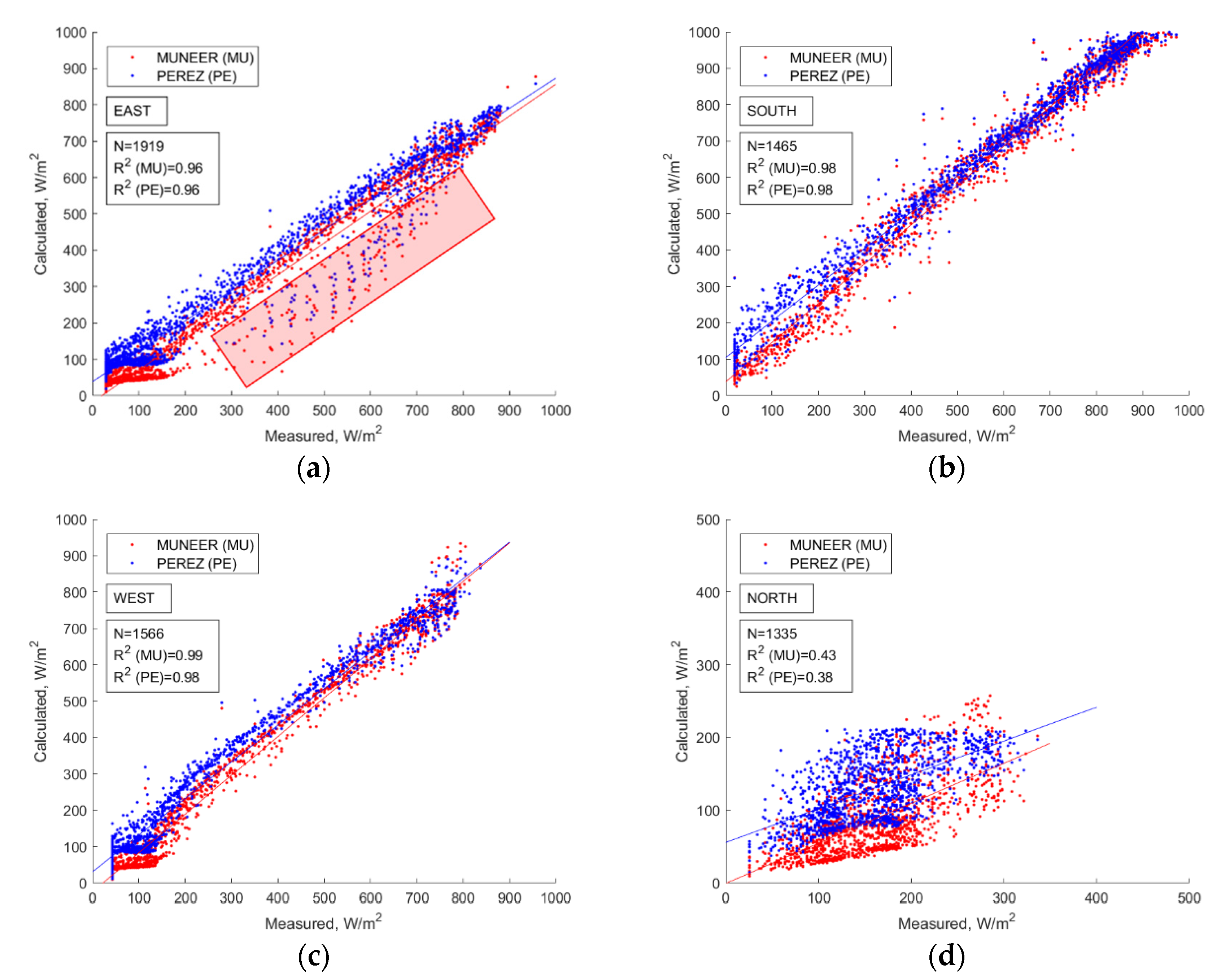
Two well-known and widely representative two and three component transposition models to estimate the in-plane irradiance on tilted surfaces were analysed in order to evaluate their performance on architectural practice and building integrated photovoltaic systems. Both use as input data the global and diffuse horizontal irradiance, which are commonly measured or can be retrieved from satellite-based estimates such as the datasets available at PVGIS tool. Estimated tilted irradiances were compared with experimental measurements recorded in Spain, NREL data measured at United States and with data obtained from PVGIS, paying special attention to the performance of the presented methodologies on vertical surfaces.

The results showed that both models present low performance at north (non-equator) facing surface, where diffuse fraction is predominant. A model which works well at any sky condition and orientation is not identified. However, both methodologies are easy, accurate enough and reliable to use for architectural designs and BIPV systems.

Regardless what methodology is chosen, there are some aspects which must be considered when it comes to urban environments, such as the contribution of ground-reflected solar irradiance, which is considered isotropic. It should be considered a key point in façade elements close to the ground since a high proportion of the incident irradiance will be due to ground reflections. Therefore, it is recommended to quantify the ground albedo coefficient by empirical evidence at the place of interest to obtain more accurate results.

Depending on the surrounding environment, it may be necessary to dismiss times with low solar elevation angles. It should be considered that under realistic conditions, there are potentially stringent limitations on applying correctly both models in an urban environment due to exposed surfaces are not commonly under completely visible sky. It should be necessary to include additional tools (3D models) that enable the user to define and position object creating a geometry for each study case and obtaining the view factor. However, the results show in this study are useful to demonstrate the upper limit of the possible solar irradiation collected by the façades facing different orientations.

Even with non-optimal orientations and tilt angles, the solar potential of PV façades reveals that the equator-facing one could receive twice as much of the solar energy that is collected by the horizontal one in winter time at the considered latitude. The sum of solar radiation received by all faces exceeds the energy collected by the horizontal one.

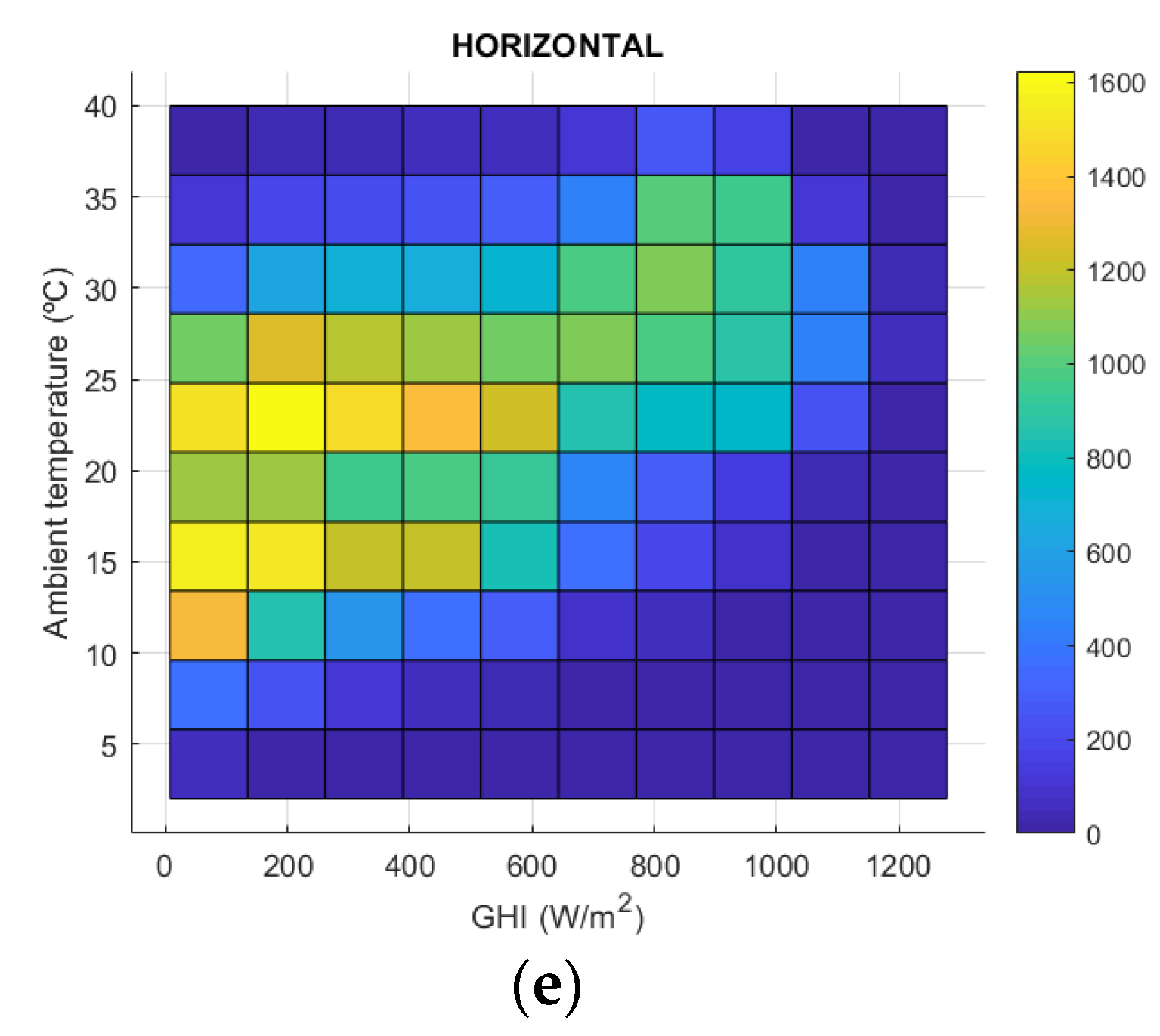
Finally, the operating condition for vertical surfaces under a full-year real working environment reveals high probability of combination of low irradiance and medium temperature, which are far from the standard test conditions (STC) commonly used to characterise PV modules.

References

1. Scognamiglio, A.; Røstvik, H.N. Photovoltaics and zero energy buildings: a new opportunity and challenge for design. Prog. Photovolt. 2013, 21, 1319–1336. [Google Scholar] [CrossRef]
2. Brito, M.C.; Freitas, S.; Guimarães, S.; Catita, C.; Redweik, P. The importance of facades for the solar PV potential of a Mediterranean city using LiDAR data. Renew. Energy 2017, 111, 85–94. [Google Scholar] [CrossRef]
3. Díez-Mediavilla, M.; Rodríguez-Amigo, M.C.; Dieste-Velasco, M.I.; García-Calderón, T.; Alonso-Tristán, C. The PV potential of vertical façades: A classic approach using experimental data from Burgos, Spain. Sol. Energy 2019, 177, 192–199. [Google Scholar] [CrossRef]
4. Redweik, P.; Catita, C.; Brito, M. Solar energy potential on roofs and facades in an urban landscape. Sol. Energy 2013, 97, 332–341. [Google Scholar] [CrossRef]
5. Vulkan, A.; Kloog, I.; Dorman, M.; Erell, E. Modeling the potential for PV installation in residential buildings in dense urban areas. Energ. Build. 2018, 169, 97–109. [Google Scholar] [CrossRef]
6. Sayyah, A.; Horenstein, M.N.; Mazumder, M.K. Energy yield loss caused by dust deposition on photovoltaic panels. Sol. Energy 2014, 107, 576–604. [Google Scholar] [CrossRef]
7. Elminir, H.K.; Ghitas, A.E.; Hamid, R.H.; El-Hussainy, F.; Beheary, M.M.; Abdel-Moneim, K.M. Effect of dust on the transparent cover of solar collectors. Energy Convers. Manag. 2006, 47, 3192–3203. [Google Scholar] [CrossRef]
8. Lu, L.; Yang, H.X. Environmental payback time analysis of a roof-mounted building-integrated photovoltaic (BIPV) system in Hong Kong. Appl. Energy 2010, 87, 3625–3631. [Google Scholar] [CrossRef]
9. Šúri, M.; Huld, T.A.; Dunlop, E.D.; Ossenbrink, H.A. Potential of solar electricity generation in the European Union member states and candidate countries. Sol. Energy 2007, 81, 1295–1305. [Google Scholar] [CrossRef]
10. Urraca, R.; Gracia-Amillo, A.M.; Koubli, E.; Huld, T.; Trentmann, J.; Riihelä, A.; Lindfors, A.V.; Palmer, D.; Gottschalg, R.; Antonanzas-Torres, F. Extensive validation of CM SAF surface radiation products over Europe. Remote Sens. Environ. 2017, 199, 171–186. [Google Scholar] [CrossRef] [Green Version]
11. EC-JRC Photovoltaic Geographical Information System (PVGIS). Available online: http://re.jrc.ec.europa.eu/pvg_tools/en/tools.html (accessed on 29 November 2018).
12. NREL PVWATTS. Available online: https://pvwatts.nrel.gov/ (accessed on 4 Feburary 2019).
13. Besharat, F.; Dehghan, A.A.; Faghih, A.R. Empirical models for estimating global solar radiation: A review and case study. Renew. Sust. Energ. Rev. 2013, 21, 798–821. [Google Scholar] [CrossRef]
14. Zhang, J.; Zhao, L.; Deng, S.; Xu, W.; Zhang, Y. A critical review of the models used to estimate solar radiation. Renew. Sustain. Energy Rev. 2017, 70, 314–329. [Google Scholar] [CrossRef]
15. Bocca, A.; Bergamasco, L.; Fasano, M.; Bottaccioli, L.; Chiavazzo, E.; Macii, A.; Asinari, P. Multiple-Regression Method for Fast Estimation of Solar Irradiation and Photovoltaic Energy Potentials over Europe and Africa. Energies 2018, 11, 3477. [Google Scholar] [CrossRef] [Green Version]
16. de Simón-Martín, M.; Alonso-Tristán, C.; Díez-Mediavilla, M. Diffuse solar irradiance estimation on building’s façades: Review, classification and benchmarking of 30 models under all sky conditions. Renew. Sustain. Energy Rev. 2017, 77, 783–802. [Google Scholar] [CrossRef]
17. Yang, D. Solar radiation on inclined surfaces: Corrections and benchmarks. Sol. Energy 2016, 136, 288–302. [Google Scholar] [CrossRef]
18. Gueymard, C.A. Direct and indirect uncertainties in the prediction of tilted irradiance for solar engineering applications. Sol. Energy 2009, 83, 432–444. [Google Scholar] [CrossRef]
19. Perez, R.; Ineichen, P.; Seals, R.; Michalsky, J.; Stewart, R. Modeling daylight availability and irradiance components from direct and global irradiance. Sol. Energy 1990, 44, 271–289. [Google Scholar] [CrossRef] [Green Version]
20. Perez, R.; Stewart, R.; Seals, R.; Guertin, T. The Development and Verification of the Perez Diffuse Radiation Model; Technical Report; Sandia National Labs: Albuquerque, NM, USA, 1 October 1988. [Google Scholar] [CrossRef]
21. Perez, R.; Seals, R.; Ineichen, P.; Stewart, R.; Menicucci, D. A new simplified version of the perez diffuse irradiance model for tilted surfaces. Sol. Energy 1987, 39, 221–231. [Google Scholar] [CrossRef] [Green Version]
22. Perez, R.; Stewart, R.; Arbogast, C.; Seals, R.; Scott, J. An anisotropic hourly diffuse radiation model for sloping surfaces: Description, performance validation, site dependency evaluation. Sol. Energy 1986, 36, 481–497. [Google Scholar] [CrossRef]
23. Muneer, T. Solar radiation model for Europe. Build Serv. Eng. Res. Technol. 1990, 11, 153–163. [Google Scholar] [CrossRef]
24. Muneer, T.; Gueymard, C.; Kambezidis, H. 4-Hourly Slope Irradiation and Illuminance. In Solar Radiation and Daylight Models (Second Edition); Muneer, T., Gueymard, C., Kambezidis, H., Eds.; Butterworth-Heinemann: Oxford, UK, 2004; p. 143. [Google Scholar]
25. Gueymard, C. An anisotropic solar irradiance model for tilted surfaces and its comparison with selected engineering algorithms. Sol. Energy 1987, 38, 367–386. [Google Scholar] [CrossRef]
26. Hay, J.E. Calculating solar radiation for inclined surfaces: Practical approaches. Renew. Energy 1993, 3, 373–380. [Google Scholar] [CrossRef]
27. Hay, J.E.; Davies, J.A. Calculation of the Solar Radiation Incident on an Inclined Surface. In Proceedings of the 1st Canadian Solar Radiation Data Workshop, Toronto, ON, Canada, 17−19 April 1980. [Google Scholar]
28. Gracia, A.M.; Huld, T. Performance Comparison of Different Models for the Estimation of Global Irradiance on Inclined Surfaces. 2013. Available online: http://publications.europa.eu/resource/cellar/4ef8c4e1-4397-4e27-8487-448786327f27.0001.01/DOC_1 (accessed on 1 December 2019).
29. Bugler, J.W. The determination of hourly insolation on an inclined plane using a diffuse irradiance model based on hourly measured global horizontal insolation. Sol. Energy 1977, 19, 477–491. [Google Scholar] [CrossRef]
30. Hay, J.E. Study of Shortwave Radiation on Non-Horizontal Surfaces; Report 79-12; Atmospheric Environment Services: Downsview, ON, Canada, 1979. [Google Scholar]
31. Skartveit, A.; Asle Olseth, J. Modelling slope irradiance at high latitudes. Sol. Energy 1986, 36, 333–344. [Google Scholar] [CrossRef]
32. Willmott, C.J. On the climatic optimization of the tilt and azimuth of flat-plate solar collectors. Sol. Energy 1982, 28, 205–216. [Google Scholar] [CrossRef]
33. Klucher, T.M. Evaluation of models to predict insolation on tilted surfaces. Sol. Energy 1979, 23, 111–114. [Google Scholar] [CrossRef]
34. Reindl, D.T.; Beckman, W.A.; Duffie, J.A. Evaluation of hourly tilted surface radiation models. Sol. Energy 1990, 45, 9–17. [Google Scholar] [CrossRef]
35. Temps, R.C.; Coulson, K.L. Solar radiation incident upon slopes of different orientations. Sol. Energy 1977, 19, 179–184. [Google Scholar] [CrossRef]
36. Stoffel, T.; Andreas, A. NREL Solar Radiation Research Laboratory (SRRL): Baseline Measurement System (BMS); National Renewable Energy Lab. (NREL): Golden, CO, USA, 1981. [Google Scholar] [CrossRef]
37. Cooper, P.I. The absorption of radiation in solar stills. Sol. Energy 1969, 12, 333–346. [Google Scholar] [CrossRef]
38. Spencer, J. Fourier Series Representation of the Position of the Sun. Search 1971, 2, 172–172. [Google Scholar]
39. Yallop, D.B. Technical Note; Royal Greenwich Observatory: Cambridge, UK, 1992. [Google Scholar]
40. Angus, R.C.; Muneer, T. Sun position for daylight models: Precise algorithms for determination. Light. Res. Technol. 1993, 25, 81–83. [Google Scholar] [CrossRef]
41. Liu, B.Y.H.; Jordan, R.C. The interrelationship and characteristic distribution of direct, diffuse and total solar radiation. Sol. Energy 1960, 4, 1–19. [Google Scholar] [CrossRef]
42. Igawa, N.; Koga, Y.; Matsuzawa, T.; Nakamura, H. Models of sky radiance distribution and sky luminance distribution. Sol. Energy 2004, 77, 137–157. [Google Scholar] [CrossRef]
43. Brunger, A.P.; Hooper, F.C. Anisotropic sky radiance model based on narrow field of view measurements of shortwave radiance. Sol. Energy 1993, 51, 53–64. [Google Scholar] [CrossRef]
44. Iqbal, M. An Introduction to Solar Radiation; Academic Press: Toronto, ON, Canada, 1983; ISBN 978-0-12-373750-2. [Google Scholar]
45. Kasten, F.; Young, A.T. Revised optical air mass tables and approximation formula. Appl. Opt. 1989, 28, 4735–4738. [Google Scholar] [CrossRef]
46. Wood, J.; Muneer, T.; Kubie, J. Evaluation of a New Photodiode Sensor for Measuring Global and Diffuse Irradiance, and Sunshine Duration. J. Sol. Energy Eng. 2003, 125, 43–48. [Google Scholar] [CrossRef] [Green Version]
47. Toledo, C.; Serrano-Lujan, L.; Abad, J.; Lampitelli, A.; Urbina, A. Measurement of Thermal and Electrical Parameters in Photovoltaic Systems for Predictive and Cross-Correlated Monitorization. Energies 2019, 12. [Google Scholar] [CrossRef] [Green Version]
48. Long, C.N.; Dutton, E.G. BSRN Global Network Recommended QC Tests. V2.0. 2002. Available online: https://bsrn.awi.de/fileadmin/user_upload/bsrn.awi.de/Publications/BSRN_recommended_QC_tests_V2.pdf (accessed on 12 December 2019).
49. WRMC Reviewed Scientific Papers Referring to BSRN. Available online: https://bsrn.awi.de/other/publications/reviewed-scientific-papers-referring-to-bsrn/ (accessed on 29 June 2019).
50. Marquez, R.; Coimbra, C.F.M. Proposed Metric for Evaluation of Solar Forecasting Models. J. Sol. Energy Eng. 2012, 135, 011016–011016. [Google Scholar] [CrossRef] [Green Version]
51. Gueymard, C.A.; Lara-Fanego, V.; Sengupta, M.; Xie, Y. Surface albedo and reflectance: Review of definitions, angular and spectral effects, and intercomparison of major data sources in support of advanced solar irradiance modeling over the Americas. Sol. Energy 2019, 182, 194–212. [Google Scholar] [CrossRef]
52. Loutzenhiser, P.G.; Manz, H.; Felsmann, C.; Strachan, P.A.; Frank, T.; Maxwell, G.M. Empirical validation of models to compute solar irradiance on inclined surfaces for building energy simulation. Sol. Energy 2007, 81, 254–267. [Google Scholar] [CrossRef] [Green Version]
53. Urraca, R.; Huld, T.; Lindfors, A.V.; Riihelä, A.; Martinez-de-Pison, F.J.; Sanz-Garcia, A. Quantifying the amplified bias of PV system simulations due to uncertainties in solar radiation estimates. Sol. Energy 2018, 176, 663–677. [Google Scholar] [CrossRef] [Green Version]
54. Hofierka, J.; Šúri, M. The solar radiation model for Open source GIS: implementation and applications. In Proceedings of the Open Source GIS-GRASS Users Conference, Trento, Italy, 11–13 September 2002; pp. 51–70. [Google Scholar]
55. Huld, T.; Dunlop, E.; Beyer, H.G.; Gottschalg, R. Data sets for energy rating of photovoltaic modules. Sol. Energy 2013, 93, 267–279. [Google Scholar] [CrossRef]
56. Kenny, R.P.; Dunlop, E.D.; Ossenbrink, H.A.; Müllejans, H. A practical method for the energy rating of c-Si photovoltaic modules based on standard tests. Prog. Photovolt. Res. Appl. 2006, 14, 155–166. [Google Scholar] [CrossRef]
57. Huld, T.; Friesen, G.; Skoczek, A.; Kenny, R.P.; Sample, T.; Field, M.; Dunlop, E.D. A power-rating model for crystalline silicon PV modules. Sol. Energy Mater. Sol. Cells 2011, 95, 3359–3369. [Google Scholar] [CrossRef]
58. Hasan, A.; McCormack, S.J.; Huang, M.J.; Norton, B. Evaluation of phase change materials for thermal regulation enhancement of building integrated photovoltaics. Sol. Energy 2010, 84, 1601–1612. [Google Scholar] [CrossRef] [Green Version]
Figure 1. Zenith angle (θz), slope (β), surface azimuth angle (γ) and solar azimuth angle for a tilted surface (γs).
Energies 13 00702 g001
Figure 2. (a) Test location at coordinates 38.02347, −1.17600; (b) Pyranometers placed on the gravel roof of a three-story building at University of Murcia; (c) Pyranometer with shadow band model Delta-T Device model BF5 to measure GHI and DHI, and Kipp&Zonen model CMP3 to measure global in-plane irradiance at different orientations.
Energies 13 00702 g002
Figure 3. Albedo measurements. (a) Two representative days at the ground station in Murcia in winter and summer season, together with median values for each day, 5-min time steps records; (b) Full-year at NREL laboratories, together with median value of 0.21, hourly-average values.
Energies 13 00702 g003
Figure 4. Correlation between calculated (based on BF5 pyranometer data) and measured (with CMP3 pyranometer) applying Perez (PE) and Muneer (MU) transposition models. (a) East; (b) South; (c) West; (d) North. Figure (a) shows high deviation between estimated and measured values, indicated by a red rectangle, generated by shadows at dawn.
Energies 13 00702 g004
Figure 5. Calculated vs. measured irradiance considering Sun elevation angles above 15°. (a) East; (b) South; (c) West; (d) North.
Energies 13 00702 g005
Figure 6. Histogram of the sky type according to Igawa et al. classification for (a) period under analysis in Spain and (b) full-year data, 2018 for NREL data.
Energies 13 00702 g006
Figure 7. Comparison of global in-plane irradiance from PVGIS and models outcomes, as well as the beam, diffuse and reflected components for a random day in Murcia, Spain. (a) East, (b) south, (c) west and (d) north orientations (GMT + 0).
Energies 13 00702 g007
Figure 8. Monthly average of daily irradiation (kWh/m2/day). PVGIS-SARAH database and measured data for the year 2018.
Energies 13 00702 g008
Figure 9. Comparison of the daily radiation profile for January from PVGIS-SARAH satellite-based database for a multi-year period (2005–2016) and from experimental measurements from in-situ ground station registered in the year 2018 at the considered location in Murcia (Spain). (a) East; (b) South; (c) West; (d) North.
Energies 13 00702 g009
Figure 10. Combination of in-plane irradiance calculated by Muneer’s method from horizontal irradiance records and ambient temperature collected at the weather station for (a) vertical east-facing surface, (b) vertical south-facing surface, (c) vertical west-facing surface, (d) vertical north-facing surface and (e) horizontal surface. Frequency of observations are plotted on the right bar where the colour scale indicates the number of observations.
Energies 13 00702 g010aEnergies 13 00702 g010b