Sensitivity Analysis of an Implanted Antenna within Surrounding Biological Environment


1
Group of Electrical Engineering, University of Paris-Saclay, CentraleSupélec, CNRS, Gif-sur-Yvette, 91192 Paris, France
2
Group of Electrical Engineering, Sorbonne University, CNRS, 75252 Paris, France
*
Author to whom correspondence should be addressed.
Energies 2020, 13(4), 996; https://doi.org/10.3390/en13040996
Submission received: 31 January 2020
/
Revised: 19 February 2020
/
Accepted: 21 February 2020
/
Published: 23 February 2020
(This article belongs to the Special Issue Intelligent Wireless Power Transfer System and Its Application)
Abstract
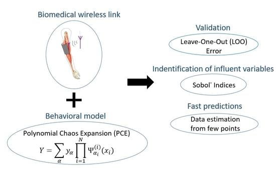
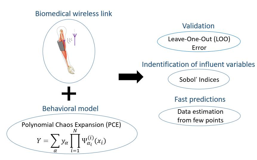
:The paper describes the sensitivity analysis of a wireless power transfer link involving an implanted antenna within the surrounding biological environment. The approach combines a 3D electromagnetic modeling and a surrogate model (based polynomial chaos expansion). The analysis takes into account geometrical parameters of the implanted antenna and physical properties of the biological tissue. It allows researchers to identify at low cost the main parameters affecting the efficiency of the transmission link.
1. Introduction
Implantable Medical Devices (IMDs) have been popularly studied recently. As the modern health care system evolves, IMDs are used frequently in order to continuously monitor personal health conditions. IMDs has the potential to be light and small and able to serve various applications. However, the huge difficulty for the utilization of IMDs is their charging since no wire could be connected to an in-body IMD. Highly integrated radio-frequency (RF) circuits and developments of wireless inductive links have a significant impact on IMDs [1,2,3]. Miniaturized antennas provide wireless communication capability to transmit signals through organs or tissues towards a receiver outside the body and/or receive commands to adjust the implant settings. They also allow continuous monitoring and therapeutic treatment without constraints to the patient’s mobility. Medical implants have the advantages of being light and small. These antennas can obtain real-time information in biomedical telemetry and transmit physiological data to the external antenna. For different purposes, they are used for body-centric communication [4], glucose monitoring [5], and other body parts of telemetry [6,7,8]. Since the charging process is always noninvasive, obtaining an optimal electromagnetic link is challenging, necessitating, among others, designation of several design parameters like operational frequency, implanted device shape, and maximum power deposited on the tissues while implant size needs to be minimal to avoid tissue damage and increase patient safety. For biomedical uses, several frequency bands are authorized: Medical Device Radiocommunication (MedRadio) Service band (401–406 MHz), and the Industrial, Scientific, and Medical (ISM) bands (433.1–434.8 MHz, 868–868.6 MHz, 902.8–928 MHz and 2.4–2.5 GHz). Also, a Radio Frequency (RF) medical energy transmission system normally consists of two parts: an antenna for receiving energy from external power source and a rectifying circuit for converting AC power to DC power [9,10,11,12].
As one of the three common methods for wireless power transfer in large scale, microwave radiation has its own advantages by operating in the farfield range: smaller and more robust to physical positioning or disorientations than two other transmission methods, and perfectly fit the requirements for an IMD. Therefore, many researches have been published with their own designs or analyses in this domain: H. Zhang et al. have designed an antenna embedded into muscle phantom at 2.4 GHz [13]; A. Kiourti et al. have also proposed and tested their design which is implanted into head model at 400 MHz [14]; the research team of A. Mohamed has studied another miniaturized antenna that is simulated in a skin box as well [15].
In [16], a miniaturized circular antenna was designed to support both energy and information transmission. The antenna is embedded into a three-layer cylindrical model of arm and its performance is evaluated. It has dual resonant frequency which covers MedRadio (401–406 MHz) and ISM bands (902–928 MHz). The wireless transmission link was analyzed and allowed to determine the amount of power that could be received from an external antenna at maximum authorized input power. However, it was observed that the performance of the implanted antenna and the characteristics of the transmission link are highly dependent on many parameters defining the electromagnetic problem. Geometrical parameters considered in the study like implantation depth, orientation of the antenna, and distance between exciting source and embedded antenna strongly affect the overall efficiency of the system. Also, physical parameters relevant to materials used for the miniaturized system or relevant to the environment (biological tissues) impact the global efficiency.
Indeed, 3D computational models can be applied for solving the global electromagnetic problem involving implanted antenna and the environment. Such full wave computational approaches give reliable results about the resulting efficiency of the transmission link, taking into account inhomogeneous materials and fine details of the implanted system. Nevertheless, any modification in the problem needs to run again the 3D simulation and in case of parametric or sensitivity analysis this may lead to heavy computational burden. In such a situation, the introduction of stochastic tools allows researchers to deal with the variability of all the parameters describing the electromagnetic problem. Such approaches were shown to be very efficient in the framework of the determination of specific rate absorption (SAR) in biological tissues due to mobile phones at microwaves frequencies [17,18,19] and more recently to electromagnetic compatibility problems [20].
This paper shows that a surrogate model based on polynomial chaos expansion (PCE) provides a powerful tool for optimizing the performances of the transmission link and perform a sensitivity analysis at low cost. In particular, such PCE gives straightforward results regarding Sobol’s indices highlighting the most significant geometrical parameters in the study.
2. Implanted Antenna Scenario and Transmission Link
In fact, many factors could affect the power transmission efficiency, especially with the presence of an extremely lossy material like human tissue. But these factors are not often studied by researchers nowadays. In this paper, a parametric uncertainty study on a biomedical wireless power transmission link is performed. As presented in Figure 1, a four-layer human arm model (bone, muscle, fat, skin) is designed and used in this electromagnetic simulation. Comparing the previous works [13,14,15], the four-layer model that is used in this paper is more realistic without taking much more time to calculate.
In this model, a miniaturized circular antenna is embedded into the muscle layer and the implantation depth is calculated from the muscle-fat interface to the antenna center. The implanted antenna is embedded along the direction of the muscle fiber in order not to hamper the arm’s movement. Table 1 shows the electrical properties of different human tissue at 915 MHz. The length of this human arm model is set to the minimum sufficient value with which the results are not affected in order to save the calculation time.
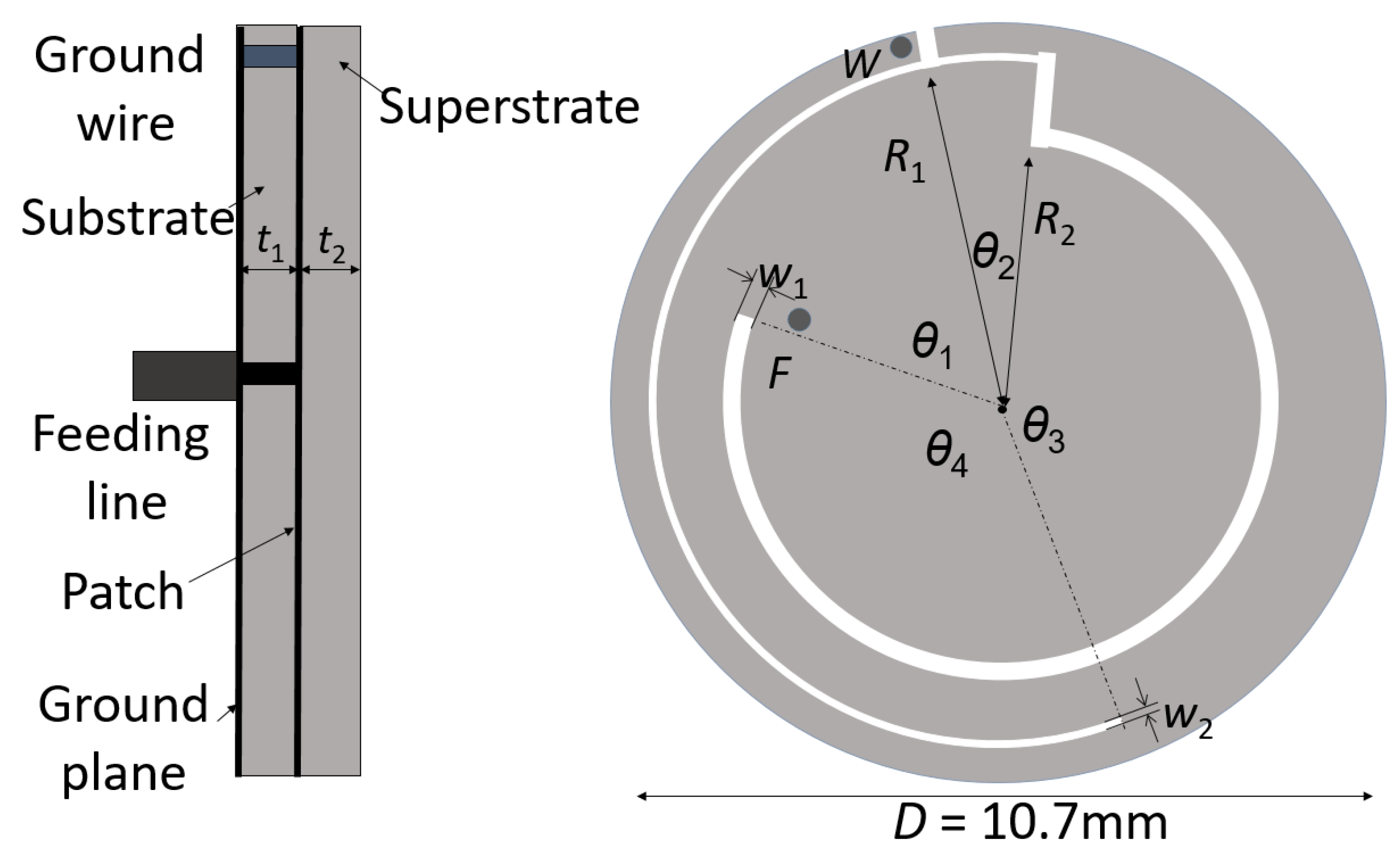
The embedded antenna with all relative parameters are presented in Figure 2. The antenna has a circular substrate (thickness = 0.64mm) and a superstrate of the same size and thickness, which are all made of material Rogers RO3210 (εr = 10.2, tanδ = 0.003). A radiating patch situates between the two layers. Two arctic slots are cut from the metallic patch for the appearance of the two resonant frequencies (400 MHz at MedRadio band and 915 MHz at ISM band respectively). A ground plane positions below the substrate and is connected with the radiating patch by a via (radius = 0.15 mm) at point W for miniaturization. A coaxial cable standardized to 50 Ω is used for feeding the antenna at point F. All the necessary parameters are marked in Figure 2 and detailed in Table 2. Due to multiple standards on the transmission power limit [21,22], this wireless power transmission system operates at the ISM bands (902.8–928 MHz) and the antenna is used for receiving power from another outside antenna at this frequency.
A metallic wave reflector is placed behind the human tissue model in order to enhance the implanted antenna’s power reception. The half-cylindrical reflector (open angle = 180°, thickness = 1.2 mm) is placed behind skin surface (see Figure 1) at the opposite to the patch antenna side. Reflector is made of copper and has a thickness larger than the penetration depth. It is cylindrical and the radius is chosen according to the following formula:
where f is the reflector’s focal distance, d is the reflector’s width and θ0 is half value of the reflector’s open angle.
In this paper, several different variables are analyzed. The thickness of the muscle and fat and the radius of the bone are all variable in order to simulate different cases of the wearing patient. Also, the implantation depth and the reflector to skin distance are also variable in order to simulate some other uncertainties such as patient’s movement or wearing clothes. All these variables and calculation are chosen according to multiple concerns for utilization in real life. Finally, the gain of the antenna inside the human arm model at 915 MHz is the output parameter.
In order to eliminate the mismatch loss impact from the output results, the reflection coefficients are calculated. As shown in Figure 3, the antenna always has a resonant frequency at 915 MHz and the corresponding S11 is around −16 dB which indicates that it is matched with the input impedance.
For all the samples that are used in Section 4, the reflection coefficient S11 is always ensured to be less than −10 dB in order to avoid the mismatch loss.
3. Polynomial Chaos Expansion (PCE)
Polynomial chaos expansion methods are non-intrusive methods and use 3D solvers as black boxes. Let M be a mathematical model that from N input values (parameters) generates the output (observable) y given by:
The input values maybe affected by some random variations or uncertainties. Assuming that the components of the input random vector X are independent, it can be shown that if the random response of the physical phenomena Y has a finite variance, then it can be expressed as an infinite modal expansion, denoted polynomial chaos:
where α is a multi-index, are the coefficients, are basis functions, multivariate orthonormal polynomials. These polynomials are built using tensor products:
where α denotes the N-uplet divided by subheadings.
These univariate polynomials are a family of orthonormal polynomials with respect to the margin probability density functions (pdf) given by:
where δjk is the Kronecker symbol.
If is the marginal pdf of the random input variable Xi, then from the independence of the input variables then the pdf of X is given by:
In case of uniform or Gaussian input distributions, the corresponding polynomial basis are the Legendre and Hermite polynomials families, respectively. The PCE coefficients can be estimated by using spectral projections or via the use of least-square regressions. The “projection” approach takes advantage of the orthogonality of the chaos polynomials [23].
Surrogate Model Based on PCE
A truncation of the Polynomial Chaos Expansion provides a surrogate model at low cost avoids if the evaluation of the coefficients is performed using least-square regressions. Let us consider an approximate model of the exact model M. The corresponding random output is given by a truncated sum of P polynomials expressed as:
The unknown coefficients of the truncation can be estimated through least square regression while minimizing a root mean square error. If we denote y the output vector collecting n values in the vector corresponding to the n inputs x(i) (i = 1,…,n) given by , then the estimated unknown coefficients derived from a regression approach are given by:
where is the matrix whose coefficients are .
The Latin Hypercube Sampling approach, known as LHS, is often used for planning the design of experiments. The validation of the truncated model can be checked using Bootstrap or LOO (Leave-One-Out) validation error. This last approach is a natural definition. If we consider n input values x(i) giving n output , one sample point can be removed and a new surrogate model can be built on the basis of n − 1 sample values. Then a comparison between the predicted output value with this surrogate model and the value can reflects the accuracy of the approach. This leads to the LOO criterion defined as:
Depending on the targeted accuracy, new samples can be added. From the computational efficacy point of view, it is important to select the most important polynomials. Then, a further reduction of the basis size can be performed using an adaptive technique, the so-called LARS algorithm (Least angle regression method) [24]. This algorithm identifies the polynomials having the most impact on the output response and on the sensibility indices.
For a sensitivity analysis the “Sobol” decomposition [25] is well known. Quantitative estimates of the output sensitivity both to each input individually and to each of possible combinations as well, are straightforward; thanks to the orthonormality of the polynomial chaos basis, the global variance and the partial variances can be expressed with the coefficients of the expansion:
where the set of α tuples such that only the indices are nonzero:
The indices can be analytically extracted from the PCE [23] and are defined as:
4. Numerical Results and Discussion
All the calculations in this chapter are performed by the UQLab module in Matlab [26]. The sample data points are obtained from simulations by CST Studio Suite [27]. In general, one group with 5 variables (radius of bone B, reflector to skin distance R, thickness of fat F, thickness of muscle M, and implantation depth I) 243 samples in total are analyzed. The chosen observable output in the electromagnetic problem is the gain of the antenna. The ranges for each variable are presented in the following Table 3. In these variable ranges, the S11 value is almost immune to changes and stays at around −16 dB.
4.1. LOO Error
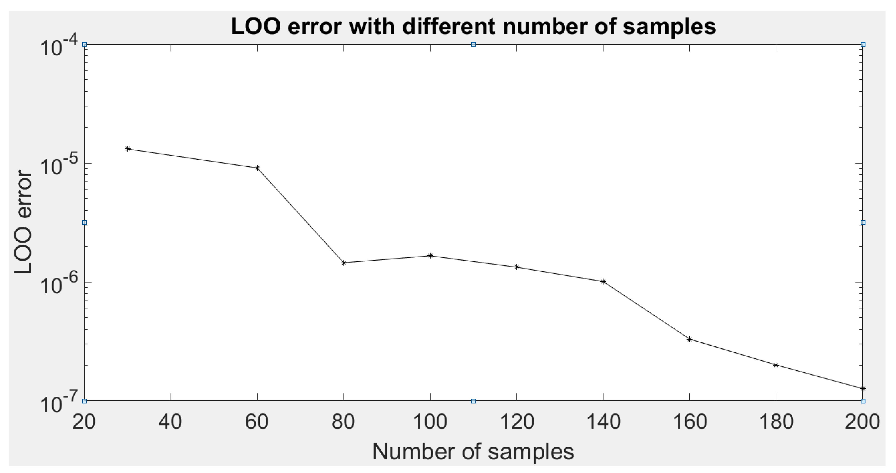
As a global indicator for the method accuracy, the LOO error of the first group of variables is shown in Figure 4.
As seen in Figure 4, the LOO error decreases effectively as more samples are included into the database. When 200 sample point are taken into account, the LOO error is 1.2 × 10⁻⁷. This validates the reliability of the established PCE model and ensure the correctness of the following results.
4.2. Sobol Indices
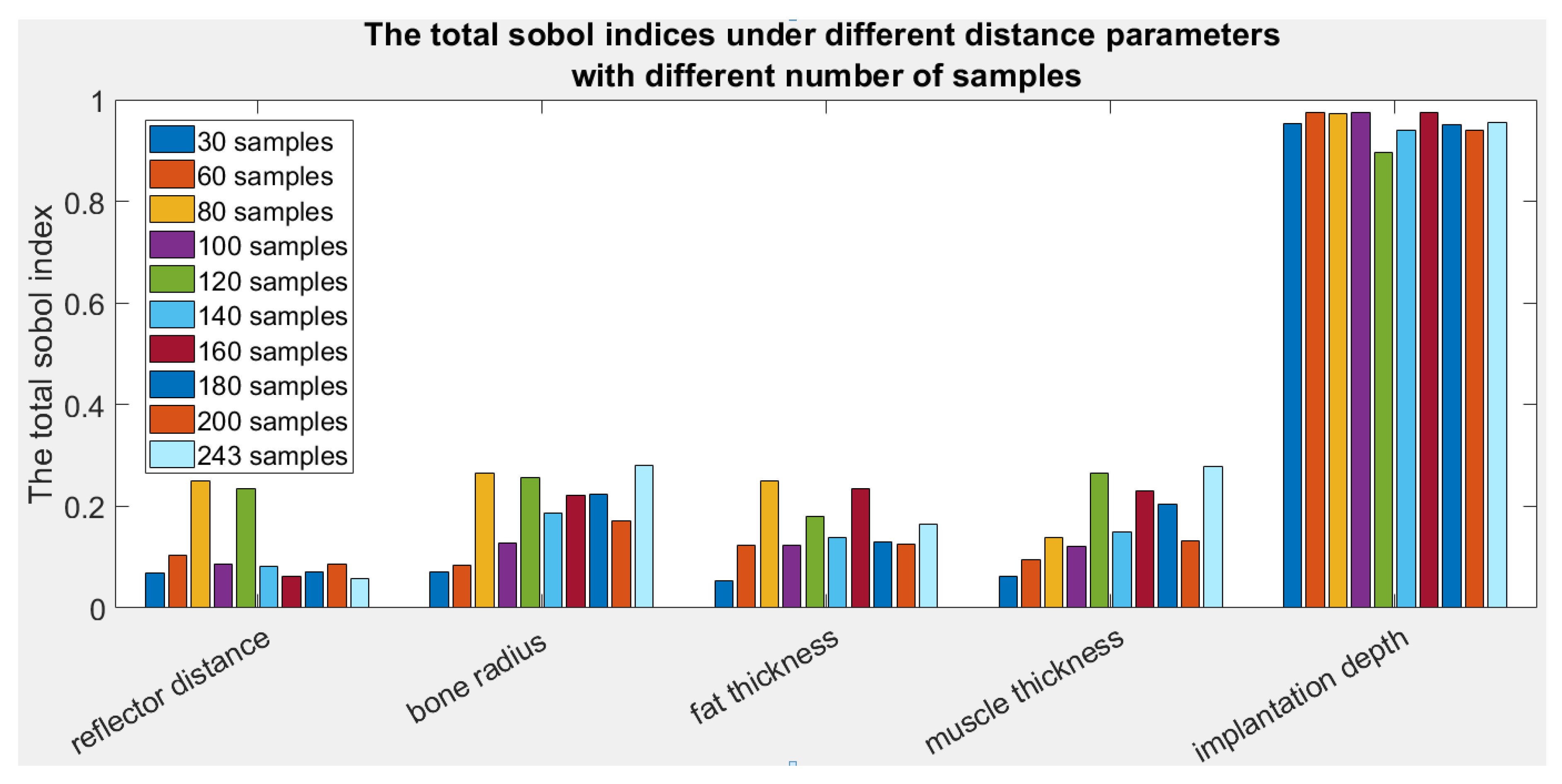
Sobol Index is a value that varies from 0 to 1 which indicates the sensitivity of the output against each parameter. More the index is close to 1, more influence this parameter has on the result. With the value of Sobol indices, it is easy to figure out the parameter that should be paid more attention and which one less attention. Each Sobol index of the output Gain = M (bone radius B, reflector distance R, fat thickness F, muscle thickness M, implantation depth I) is defined as
where P is one of the variables (B, R, F, M, I) that affect the output.
The Sobol indices are easy to evaluate with a surrogate PCE model by using Matlab. Figure 5 shows the first order Sobol Index relevant to the different uncertainty parameters.
As shown in Figure 5, the implantation depth is the most important factor among the five different parameters. It is worth pointing out that the implantation depth refers to the distance between the muscle-fat interface and the antenna center. This conclusion could be deduced even with only 30 samples. Therefore, the implantation depth should always be considered during the design and analyze for a wireless power transmission system.
4.3. Data Prediction
Another tremendous advantage of using PCE metamodel is that it could predict data points by using only limited numbers of sample points. This could reduce largely the calculation time, especially when the calculation model is complicated or a great number of calculations are needed. In Section 4.1, the LOO error value shows that the estimation model could be established with at least 30 samples (LOO error less than 1‰). Here, an estimation model is built basing on 60 samples in order to be more accurate. In Table 4, some random data points (except for the 60 that build the estimation model) are estimated by using the PCE model and compared with the values that calculated by CST Studio. The absolute errors and relative errors are calculated and presented in Table 4. The test sample vector is (bone radius B, reflector distance R, fat thickness F, muscle thickness M, implantation depth I).
As presented in Table 4, the five randomly chosen points are well estimated with an average relative error around 1.3%. Therefore, this surrogate model established by 60 samples could be used to estimate the real simulation results with an error tolerance less than 2%.
5. Conclusions
This paper presents a methodology based on a surrogate model (PCE method) to improve the microwave transmission link calculation in a biomedical application involving an implanted antenna. Firstly, the transmission scenario and the embedded antenna design are presented. Then the PCE method and the construction of a surrogate model based on PCE are discussed in details. With this method, the surrogate model of the transmission link is established. The trustworthiness of the model is firstly validated by LOO error and the impact of the different variables on the results is compared by calculating the Sobol indices of these variables. The result of finding that the implantation depth is the most important factor is also theoretically reasonable since the muscle tissue has a higher permittivity and thus leads to more loss. Finally, a surrogate model that is based on limited number of samples is used to estimate the results of other variable combinations. The average relative error could be easily controlled within 2% by using less than 1/4 of all samples, which proves the possibility of saving largely the calculation time by using this method when the model is relatively complex and a great number of calculation is needed. Such approach is an engineering oriented tool which may improve the design of wireless power transfers in a biomedical scenario.
Author Contributions
Conceptualization, S.D.; L.P.; methodology, L.P.; software, S.D.; validation, S.D.; L.P.; formal analysis, S.D.; investigation, S.D.; resources, S.D.; data curation, S.D.; writing—original draft preparation, S.D.; L.P.; writing—review and editing, S.D.; L.P.; visualization, S.D.; supervision, L.P.; project administration, L.P. All authors have read and agreed to the published version of the manuscript.
Funding
This research received no external funding.
Conflicts of Interest
The authors declare no conflict of interest.
References
- Kiourti, A.; Nikita, K.S. A review of implantable patch antennas for biomedical telemetry: Challenges and solutions. IEEE Antennas Propag. Mag. 2012, 54, 210–228. [Google Scholar] [CrossRef]
- Campi, T.; Cruciani, S.; Palandrani, F.; De Santis, V.; Hirata, A.; Feliziani, M. Wireless Power Transfer Charging System for AIMDs and Pacemakers. IEEE Trans. Microw. Theory Tech. 2016, 64, 633–642. [Google Scholar] [CrossRef]
- Basar, M.R.; Ahmad, M.Y.; Cho, J.; Ibrahim, F. An Improved Wearable Resonant Wireless Power Transfer System for Biomedical Capsule Endoscope. IEEE Trans. Ind. Electron. 2018, 65, 7772–7781. [Google Scholar] [CrossRef]
- Hall, P.S.; Hao, Y. Antennas and Propagation for Body-Centric Wireless Communications; Artech House: Norwood, MA, USA, 2006. [Google Scholar]
- Karacolak, T.; Hood, A.; Topsakal, E. Design of a dual-band implantable antenna and development of skin mimicking gels for continuous glucose monitoring. IEEE Trans. Microw. Theory Tech. 2008, 56, 1001–1008. [Google Scholar] [CrossRef]
- Huang, F.-J.; Lee, C.-M.; Chang, C.-L.; Chen, L.-K.; Yo, T.-C.; Luo, C.-H. Rectenna application of miniaturized implantable antenna design for trible-band biotelemetry communication. IEEE Trans. Antennas Propag. 2011, 59, 2646–2653. [Google Scholar] [CrossRef]
- Liu, C.; Guo, Y.; Sun, H.; Xiao, S. Design and safety considerations of an implantable rectenna for far-field wireless power transfer. IEEE Trans. Antennas Propag. 2014, 62, 5798–5806. [Google Scholar] [CrossRef]
- Liu, C.; Zhang, Y.; Liu, X. Circularly Polarized Implantable Antenna for 915 MHz ISM-Band Far-Field Wireless Power Transmission. IEEE Antennas Wirel. Propag. Lett. 2018, 17, 373–376. [Google Scholar] [CrossRef]
- Cheng, H.; Yu, T.; Luo, C. Direct current driving impedance matching method for rectenna using medical implant communication service band for wireless battery charging. IET Microw. Antennas Propag. 2013, 7, 277–282. [Google Scholar] [CrossRef]
- DeLong, B.J.; Kiourti, A.; Volakis, J.L. A Radiating Near-Field Patch Rectenna for Wireless Power Transfer to Medical Implants at 2.4 GHz. IEEE J. Electromagn. RF Microw. Med. Biol. 2018, 2, 64–69. [Google Scholar] [CrossRef]
- Okba, A.; Takacs, A.; Aubert, H. Compact Rectennas for Ultra-Low-Power Wireless Transmission Applications. IEEE Trans. Microw. Theory Tech. 2019, 67, 1697–1707. [Google Scholar] [CrossRef]
- Bakogianni, S.; Palaiologos, M.; Koulouridis, S. Performance evaluation and sensitivity analysis of a novel rectenna system for deep implanted devices. In Proceedings of the 2017 11th European Conference on Antennas and Propagation (EUCAP), Paris, France, 19–24 March 2017. [Google Scholar]
- Zhang, H.; Gao, S.; Ngo, T.; Wu, W.; Guo, Y. Wireless Power Transfer Antenna Alignment Using Intermodulation for Two-Tone Powered Implantable Medical Devices. IEEE Trans. Microw. Theory Tech. 2019, 67, 1708–1716. [Google Scholar] [CrossRef]
- Kiourti, A.; Nikita, K.S. Miniature scalp-implantable antennas for telemetry in the MICS and ISM bands: Design, safety considerations and link budget analysis. IEEE T. Antenn. Propag. 2012, 60, 3568–3575. [Google Scholar] [CrossRef]
- Mohamed, A.E.; Sharawi, M.S. Miniaturized dual-wideband circular patch antenna for biomedical telemetry. In Proceedings of the 2017 11th European Conference on Antennas and Propagation (EUCAP), Paris, France, 19–24 March 2017; pp. 1027–1030. [Google Scholar]
- Ding, S.; Koulouridis, S.; Pichon, L. A Dual-Band Miniaturized Circular Antenna for Deep in Body Biomedical Wireless Applications. In Proceedings of the 13th European Conference on Antennas and Propagation (EuCAP), Krakow, Poland, 31 March–5 April 2019. [Google Scholar]
- Silly-Carette, J.; Lautru, D.; Wong, M.-F.; Gati, A.; Wiart, J.; Fouad Hanna, V. Variability on the Propagation of a Plane Wave Using Stochastic Collocation Methods in a Bio Electromagnetic Application. IEEE Microw. Wirel. Compon. Lett. 2009, 19, 185–187. [Google Scholar] [CrossRef]
- Liorni, I.; Parazzini, M.; Fiocchi, S.; Ravazzani, P. Study of the Influence of the Orientation of a 50-Hz Magnetic Field on Fetal Exposure Using Polynomial Chaos Decomposition. Int. J. Environ. Res. Public Health 2015, 12, 5934–5953. [Google Scholar] [CrossRef] [PubMed] [Green Version]
- Voyer, D.; Musy, F.; Nicolas, L.; Perrussel, R. Probabilistic methods applied to 2D electromagnetic numerical dosimetry. Compel Int. J. Comput. Math. Electr. Electron. Eng. 2008, 27, 651–667. [Google Scholar] [CrossRef] [Green Version]
- Larbi, M.; Stievano, I.S.; Canavero, F.G.; Besnier, P. Variability Impact of Many Design Parameters: The Case of a Realistic Electronic Link. IEEE Trans. Electromagn. Compat. 2018, 60, 34–41. [Google Scholar] [CrossRef]
- International Telecommunications Union. Recommendation ITU-R RS.1346; ITU: Geneva, Switzerland, 1998. [Google Scholar]
- FCC. Standard Specification for Radiated Emission Limits, General Requirements; FCC 15. 209; FCC: Washington, DC, USA, 1990.
- Sudret, B. Global sensitivity analysis using polynomial chaos expansions. Reliab. Eng. Syst. Saf. 2008, 93, 964–979. [Google Scholar] [CrossRef]
- Blatman, G.; Sudret, B. Adaptive sparse polynomial chaos expansion based on least angle regression. J. Comput. Phys. 2011, 230, 2345–2367. [Google Scholar] [CrossRef]
- Sobol, I.M. Sensitivity estimates for nonlinear mathematical models. Math. Model. Comput. Exp. 1993, 1, 407–414. [Google Scholar]
- Marelli, S.; Sudret, B. UQLab: A framework for uncertainty quantification in Matlab. In Proceedings of the 2nd International Conference on Vulnerability, Risk Analysis and Management (ICVRAM2014), Liverpool, UK, 24 April 2014; pp. 2554–2563. [Google Scholar]
- Computer Simulation Technology (CST). STUDIO SUITE; Ver 2017, CST AG; CST: Danvers, MA, USA, 2017. [Google Scholar]
Figure 1.
Power transmission link design.
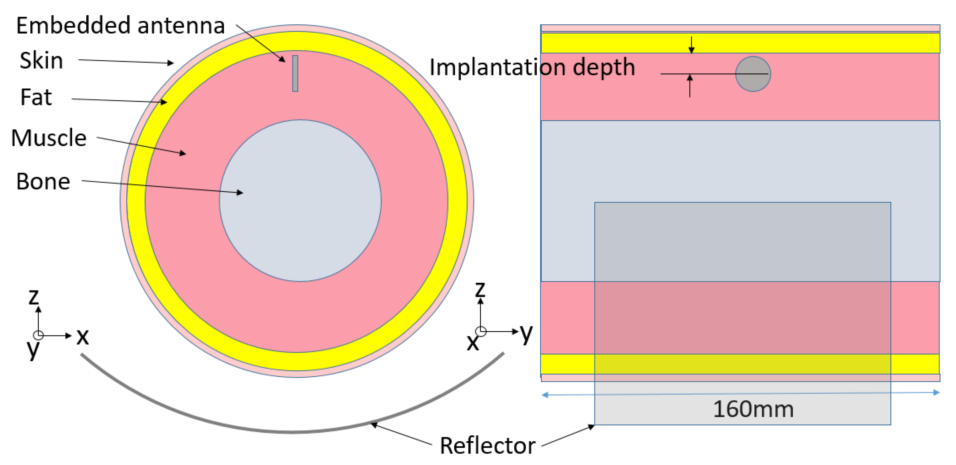
Figure 2.
Detailed antenna design.

Figure 3.
Reflection coefficient of the antenna embedded in the arm model.
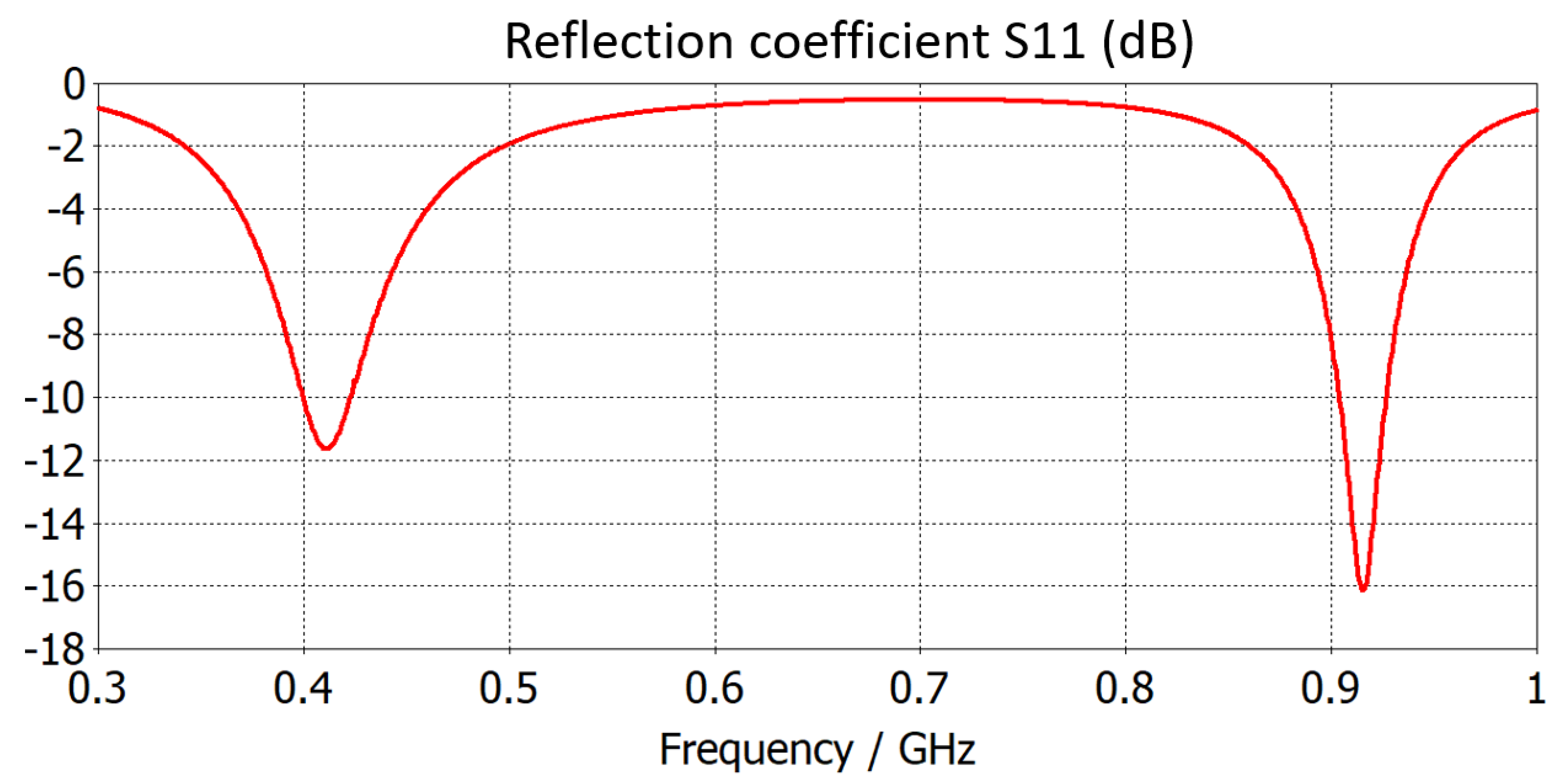
Figure 4.
Leave-One-Out (LOO) Error in log VS Number of samples.

Figure 5.
The Sobol indices VS different parameters under different number of samples.

Table 1.
Dielectric constants of human tissue.
| Frequency | Bone | Muscle | Skin | Fat | |
|---|---|---|---|---|---|
| 915 MHz | εr | 12.45 | 54.98 | 41.35 | 5.46 |
| σ (S/m) | 0.15 | 0.93 | 0.85 | 0.10 | |
Table 2.
Antenna parameters.
| Parameter Name | Value (mm) | Parameter Name | Value (mm) | Parameter Name | Value (deg) |
|---|---|---|---|---|---|
| R1 | 4.9 | t1 | 0.64 | θ1 | 70 |
| R2 | 3.76 | t2 | 0.64 | θ2 | 18 |
| w1 | 0.15 | D | 10.7 | θ3 | 163 |
| w2 | 0.32 | - | - | θ4 | 109 |
Table 3.
The ranges for the 5 analyzed variables.
| Parameter Name | Bone Radius B | Reflector to Skin Distance R | Fat Thickness F | Muscle Thickness M | Implantation Depth I |
|---|---|---|---|---|---|
| Range (mm) | 20–40 | 0–20 | 1–20 | 25–40 | 10–20 |
Table 4.
Estimation error at random points.
| Test Samples (B, R, F, M, I) (mm) | Simulated Gain (dB) | Estimated Gain (dB) | Absolute Error (dB) | Relative Error (%) |
|---|---|---|---|---|
| (10; 30; 10.5; 37.5; 15) | −29.7364 | −29.4675 | 0.268919 | 0.9043 |
| (10; 36.67; 10.5; 37.5; 15) | −29.0338 | −28.6122 | 0.421595 | 1.4521 |
| (3.3; 30; 10.5; 27.5; 11.67) | −27.8142 | −27.5534 | 0.260767 | 0.9375 |
| (10; 23.33; 10.5; 37.5; 15) | −28.7928 | −29.253 | 0.460239 | 1.5985 |
| (16.67; 0; 10.5; 32.5; 15) | −28.2000 | −28.6401 | 0.440114 | 1.5607 |
© 2020 by the authors. Licensee MDPI, Basel, Switzerland. This article is an open access article distributed under the terms and conditions of the Creative Commons Attribution (CC BY) license (http://creativecommons.org/licenses/by/4.0/).
Share and Cite
MDPI and ACS Style
Ding, S.; Pichon, L. Sensitivity Analysis of an Implanted Antenna within Surrounding Biological Environment. Energies 2020, 13, 996. https://doi.org/10.3390/en13040996
AMA Style
Ding S, Pichon L. Sensitivity Analysis of an Implanted Antenna within Surrounding Biological Environment. Energies. 2020; 13(4):996. https://doi.org/10.3390/en13040996
Chicago/Turabian StyleDing, Shuoliang, and Lionel Pichon. 2020. "Sensitivity Analysis of an Implanted Antenna within Surrounding Biological Environment" Energies 13, no. 4: 996. https://doi.org/10.3390/en13040996
Note that from the first issue of 2016, this journal uses article numbers instead of page numbers. See further details here.