Regulated Emissions of Biogas Engines—On Site Experimental Measurements and Damage Assessment on Human Health

Abstract

Despite biogas renewability, it is mandatory to experimentally assess its combustion products in order to measure their pollutants content. To this purpose, the Authors selected six in-operation biogas plants fed by different substrates and perform an on-site experimental campaign for measuring both biogas and engines exhausts composition. Firstly, biogas measured compositions are compared among them and with data available in literature. Then, biogas engines’ exhaust compositions are compared among them, with data available in literature and with measurements obtained from an engine characterised by the same design power but fuelled with natural gas. Finally, the Health Impact Assessment analysis is used to estimate the damage on human health caused by both biogas and natural gas engines emissions. Results show that biogas causes a damage on human health three times higher than the natural gas one. But, this approach does not consider biogas renewability. So, to include this important aspect, also an analysis which considers Global Warming categories is carried out. Results highlight that natural gas is twice harmful than biogas.

1. Introduction

By now, it is a matter of fact that, despite the $279.8 billion of global investment in renewable energy sources [1] and after three flat years, global energy-related Carbon Dioxide (CO₂) emissions rose by 1.6% [2].

The rise in CO₂ emissions, the continue growth of global primary energy consumption (+2.2%) [1], the millions of premature death each year caused by energy related air pollution [2] and the expected increment of world population of an additional 1.7 billion by 2040 which can additionally push up the world energy demand by more than a quarter [2] are factors which contributes to veer away from the climate targets. Therefore, there is an urgent need of new energy policies and global environmental protection actions.

As known, since the second half of the 90’s, the world authorities are working on worldwide treaties devoted to GreenHouse Gas (GHG) emissions reduction in view of the fact that global warming is taking place and the main cause is the anthropic CO₂ emissions.

The Kyoto protocol [3] was the first international treaty while Paris Agreement [4] was the second.

Despite the adoption of the Kyoto Protocol date back to 1997, the treaty entered into force only on 16 February 2005, while its end is scheduled for 2020; the year in which the Paris Agreement, adopted by consensus on 12 December 2015, will enter into force.

Global treaties are not the unique and most effective actions put into practice because the members of the European Union (EU) fixed, since 2009, binding objectives for 2020 [5], 2030 [6] and 2050 [7].

For 2020, a 20% reduction of GHG emissions based on 1990 levels, a 20% of energy coming from Renewable Energy Sources (RES) and a rise of 20% of energy efficiency are set as common targets. Common goals are the result of the yearly purposes set for each member state and renewable resources. By means of a National Renewable Energy Action Plan (NREAP), each member state established commitments and initiatives put into force by the Country to fulfil the fixed overall targets and the objectives for RES, heating and cooling, electricity and transport as well as the support polities.

For 2030, the expected reduction of GHG emissions on 1990 bases is equal to 40% while a target of 27% is set for both energy saving and energy consumption produced from RES.

Finally, for 2050, only a challenging objective is set up: a cut of 80% of GHG emissions from 1990 levels.

Even though the Kyoto protocol is in force, the 70% of global net additions are renewable based power and the explosive annual growth of wind and solar installed capacity (+21% and +47%, respectively, in 2017), CO₂ emissions and air pollutions continue to rise as well as people awareness. Issues strictly connected to energy systems structure: still in 2017, about 85% of the world primary energy consumption (13,511.2 Mtoe) is covered by fossil fuels: 34.2% using oil, 27.6% adopting coal and 23.4% utilizing natural gas [1].

However, analysing the period 2007–2017, an encouraging and unexpected event occurred: fossil fuels quota dropped from 92% to 85% despite the primary energy consumption continues to move upward under the push of in-developing countries economic growth.

In particular, the non-OECD (non-Organization for Economic Co-operation and Development) countries primary energy consumption rose from 5897.5 Mtoe to 7906.1 Mtoe while the OECD one shrank from 5693.9 Mtoe to 5605.0 Mtoe [1]. The great merit of this reduction must be assigned to EU members. Thanks to established energy policies, EU is the only region where primary energy consumption and CO₂ emissions are significantly reduced—from 1823.9 Mtoe to 1689.2 Mtoe (period 2007–2017) and of 9.4% (period 2005–2016), respectively. Optimistic results that demonstrate the effectiveness of energy policies focused on spreading the electricity production from renewable resources like wind and solar.

Notwithstanding wind and solar global potential and future contribution to electricity demand coverage, their changeable and unforeseeable nature affects their own power production. Then, it results variable in space as well as on minutes, hours, days or even months time scale. Drawback that can provoke mismatch between power supply and demand which in turns can result in management and control problems, devices fault or, even worse, from local to global blackout. Obviously, these issues can be easily solved developing and installing large-scale energy storage plants (see, e.g., References [8,9,10,11,12,13,14,15,16]) and managing properly fossil fuels power units in order to avoid components life-time reduction (see, e.g., References [17,18,19,20,21,22,23]). Independently to these facts, wind and solar can not guarantee a both stable and programmable production as well as a simultaneous generation of electricity and heat/cold: strengths of plants working with bioenergy as input.

It is undoubtedly that a widespread use of bioenergy can be the source of:

• Food security problems [24,25,26]. The competition between food and fuel is the source of great concerns because there is the risk that agricultural crops are redirected to biofuels production instead of food purposes. Aspect that can worsen the situation of poverty and food shortage in regions like the sub-Saharan Africa or in in-developing Countries.
• Soil inappropriate usage. Massive financial supports to energy crops growth to biofuels production is the second source of concerns because it can force indirect land and output use, loss of natural habitats and extensive adoption of fertilizers and pesticides to boost crops growth and, indeed, their production (see, e.g., References [27,28,29,30,31,32]).
• Environmental issues. The spread of a large number of plants fed by bioenergy is, on the one hand, absolutely desirable because it can help in the reduction of grid congestions, exploitation of local resources as well as the diffusion of hybrid systems (e.g., References [33,34]). But, on the other hand, a massive number of bioenergy plants can be the source of concerns for local communities. In several cases, people living close to these plants demonstrated concerns and fear about emissions coming from plant chimney.

In this respect, several researchers are working on bionergy potential estimation, support polices able to guarantee a sustainable development, high efficiency power generation units and technologies devoted to electricity, heat or both of them generation by means of large quantities of unused bio-wastes and bio-residues coming from forestry, agriculture or other similar fields. The energy enhancement of residues and wastes is considered a key asset that can play a key role in future energy scenarios of both developed and in-developing countries.

In particular, being solid, liquid and gaseous biofuels (e.g., wood, bioethanol, biodiesel, vegetable oil, biogas, biomethane, etc.) available worldwide and able to guarantee a stable and programmable production of heat and cold, electricity or a combination of them, they can be an opportunity at local and regional level to improve/reinforce energy security, develop markets, boost employment, support economic development and, consequently, reduce poverty without stepping up power systems carbon footprint.

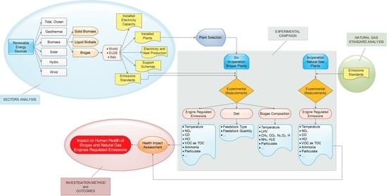
Starting from this last remark and focusing on biogas power generation plants, the authors are interested in evaluating real biogas units environmental impact with respect to both the Italian legislation and the direct fossil fuel competitor—natural gas. After that, using the Health Impact Assessment (HIA) approach, the Disability-Adjusted Life Years (DALY) is computed for both biogas and natural gas pollutants and, then, compared with amounts computable from previous published works. In this manner, a clear view of local impact on human health of pollutants coming from plants chimney can be derived and used to alleviate communities concerns about biogas plants emissions.

To foster the novelty of the work, the authors consider six in-operation biogas units fed by different feedstocks and an in-line natural gas plant. To the authors’ knowledge, no one has performed or presented a similar work in terms of both analysed plants and adopted methodology.

Biogas and natural gas are combusted in Internal Combustion Engines (ICEs) to generate heat and mechanical work; the latter is then converted into electricity. The entire set of ICEs are designed and managed by the same manufacturer and are characterised by a thermal (P_th) and electrical (P_el) power of 2459 kW and 999 kW, respectively.

Since Italian Legislation sets limits for Nitrogen Oxides (NO_x), Carbon Monoxide (CO), Hydrogen Chloride (HCl) and Volatile Organic Compounds (VOCs) expressed as Total Organic Carbon (TOC) for biogas while it restricts Particulate (PM), NO_x and Sulphur Oxide (SO_x) emissions for natural gas, Authors consider these substances in their comparisons and DALY computations.

The work is focused on biogas power generation technology and in Section 2 a brief overview of renewable and biogas sectors are presented considering the world, EU and Italian status. Then, in Section 3, the available research conducted on biogas engines emissions is presented while in Section 4, the Italian Standards set for biogas engines is discussed. Section 5 describes the analysed biogas facilities while Section 6 presents the material and methods adopted during the investigation. The results are presented and discussed in Section 7 while concluding remarks and future works are given in Section 8.

2. From Renewables to Biogas: A Brief Overview of Their Status

A biofuel, which can be solid (e.g., pellets, wood chips, biomass briquettes, etc.), liquid (e.g., bioethanol, biodiesel, etc.) or gaseous (biogas and syngas), is a combustible substance obtained from biomass. Biomass, which is organic matter derived from plants, animals, and their byproducts, is the source of bioenergy or, better, it is a renewable source of energy. In fact, the combustion process of biomass generates energy in the form of heat, electricity or both [35,36,37].

Since 2000, renewables contribute for about 12–14% to world total primary energy supply and cover about 17–18% of the global gross final energy consumption [38].

With regards to 2016, RES contribution to total primary energy supply was 80.6 EJ out of 576 EJ which means 14%. An asset that placed RES in fourth position after oil (32%), coal (27%), natural gas (22%) and before nuclear energy (5%) [38]. However, the continental distribution provides a different picture because the highest RES contribution is given in Africa (48.8%) while the lower in Europe (10.5%).

In 2016, RES input to gross final energy consumption reached 66 EJ out of 368 EJ. So, with 17.9%, RES remained the fourth source even if its input was very close to the one provided by coal and natural gas (21% each) and much higher than the one given by nuclear one (2%). Only oil, which led the ranking with 38%, was really far from RES [38].

As for total primary energy supply, the regional distribution point out, again, a large penetration of RES in Africa’s gross final energy consumption (57.1%). In particular, RES was at the ranking top followed by oil (28.4%), natural gas (8.1%) and coal (6.3%). In Asia and Americas, RES stood at 15.6% while, in Europe, the contribution was equal to 13.6%. Thanks to energy efficiency polices, European gross final energy consumption was 26% lower than the Americas (70.8 EJ vs. 89.1 EJ) and less than half of the Asia one (70.8 EJ vs. 159 EJ).

By the way, looking deeper 2016 global available data [38], it can be observed that:

• Gross final energy consumption. Renewables share, equal to 17.9%, was the sum of a 13% coming from biomass, a 3% from hydro, 0.8% from wind, 0.6% from geothermal, and 0.3% and 0.1% coming, respectively, from solar and other RES. This means that biomass was the fourth contributor after oil (38%), coal (21%) and natural gas (21%).
• Total primary energy supply. RES percentage, which was equal to 14%, was the sum of 9.8% from biomass, 2.5% from hydro, 0.6% from both geothermal and wind while the rest was solar (0.5%) and tidal, ocean, and so forth. Then, 70% of the total primary energy supply from RES was accountable to biomass, while globally it was, again, in the fourth position with 9.8% after oil (32%), coal (27%) and natural gas (22%).

It is a mater of fact that biomass is a key source but, how it contributes to electricity and heat generation compared to other renewables? And, which is the role of biogas?

As clearly shown in Figure 1a, global RES electricity generation continuous to rise with an annual growth higher than 5%. But, looking the year 2016, biomass contribution to RES electricity production reached the 9% while hydro-power and wind achieved double digits percentage of growth: +68% and +16%, respectively. Solar photovoltaic (PV) remained in the fourth place with +6%.

At regional level (see Figure 2a), electricity from RES was mainly exploited in Asia (39%), Americas (33%) and Europe (26%) but, in all cases, over the 50% of that was derived from hydro while biomass stood in the third place after wind.

Focusing on electricity generation from biomass (Figure 1b), it is undoubtedly that the main contribution was given by solid biomass with over 65%. Biogas ranked second with 15.5% followed by municipal solid waste (13.5%). So, at worldwide level, biogas was the second biofuel used to generate electricity after solid biomass. A key role that can be even more clear if the regional distribution presented in Figure 2b is analysed.

In Americas and Asia solid biomass was, in practice, the only biofuel used to electricity purposes with over 78.4% and 79.6%, respectively, while, in Europe, due to the establishment of energy polices, solid biomass share rose up (43.8%) at the expense of biogas (29.5%) and municipal solid waste (20.7%) in a view of exploiting and enhancing local plants and animal residues, unused bio-refuse, municipal and industrial waste, and so forth. A fundamental aspect also to put into practice the distributed generation concept but, as already said, a source of concerns and fear for local communities about emissions coming from plants chimney.

Regarding heat generation from renewables, there is no doubt that biomass was, practically, the unique adopted source (Figure 3a) while, in terms of biofuels (Figure 3b), the vast majority came from solid biomass followed by municipal and industrial wastes. In this case, biogas played a marginal role because, usually, it is burnt in internal combustion engines to generate electricity and not, for example, in boilers to heating purposes [39,40,41].

Biogas heat quota came from the small amount of heat recovered from ICEs cooling water and oil lubrication system used to warm up digesters. Exhausts heat content is usually wasted because biogas ICEs are not equipped with waste heat recovery units (WHRUs) which use combustion products heat content to produce useful heat (e.g., hot water, steam, oil, etc.), electricity or both of them (by means of, for example, organic Rankine cycle (ORC)). Nevertheless, it is important to point out that biogas units are usually located in isolated areas where it is difficult to find a thermal user with a sufficiently constant annual thermal demand. So, there is a great unexplored potential on biogas plants in terms of waste heat which requires specific support actions to be recovered and enhanced [39,42].

Another important point can be inferred from Figure 4. At regional level, Europe was the leading region in biomass exploitation for heating purposes due to energy policies devoted to boost technologies which use municipal and industrial wastes and, in minor quota, biogas.

Before analysing European biogas sector, it is worth to remark the importance of this work for both bioenergy and biogas sectors, because findings from emissions analysis and their impact on population in terms of DALY are crucial points which can be taken into account by Governments during source boosting process as well as by local administrations in a view of improving plant acceptance by people living in its nearby.

From 2008 to 2017, global biogas generation capacity is growth from 6699 MW to 16,915 MW [43]. But, this growth was not uniformly distributed neither around the world nor within regions: Asia and Europe, leaded respectively by China and Germany grew from 83 to 1115 MW and from 4474 to 12,064 MW, respectively. Italy comes third in the EU28 after Germany and United Kingdom (UK) with 1171 MW. Therefore, biogas production has gained a considerable momentum over the last 9 years only in these two regions.

Considering the Installed Electricity Capacity (IEC), EU28 [44] is the world sector leader with 9985 MW and 17,662 biogas plants [45] followed by USA: 977 MW of IEC and over 2200 biogas units [46]. Then, Europe, and in particular EU28 [44], is the leading region in biogas sector.

From 2009 to 2016, the number of EU28 biogas plants rose from 6227 to 17,662. The sky-rocket growth rate was registered in the period 2009–2010 (+69%) while in 2010–2011, 2011–2012 and 2013–2014 also double digits increment were registered but with less impressive rates: +18%, +11% and +15%.

In 2010–2016, the IEC and the electricity generation grew respectively from 4158 MW to 9985 MW and from 31,818 GWh to 60,922 GWh, while the highest growth rates were for both reached in 2011–2012 and equal to +52% and +77%, respectively.

Based on available data [45], EU28 yearly IEC objectives were beaten every year as clearly shown in Figure 5. A fact that reveals the effectiveness of implemented support actions.

Analysing the 2016 biogas status of EU28, the 70.7% of installed plants were fed by agricultural feedstock (namely energy crops), agricultural residues (like manure, straw, etc.) and cover/catch crops (see Figure 6a). As clearly shown in Figure 6b,c, these plants constituted the 63.6% of IEC and produced the 72.1% of the electricity coming from biogas.

Referring again to Figure 6, sewage based plants were the 16.1% while the ones fed with landfill were the 9.1%. Despite the lower number, landfill based plants constituted the 21.8% of the IEC and produced the 13.2% of the total amount of electricity generated from biogas. Sewage units contribution was equal to 5.2% of the electricity and represented the 8.2% of the IEC.

Plants fed by various types of organic waste such as bio- and municipal waste, household waste and industrial waste (namely “Other” in Figure 6) were, in number, the 3.9%, contributed for 3.2% to electricity generation and represented the 6.2% of the IEC.

For the remaining plants, no information on feedstocks nature was given (namely “Unknown” in Figure 6). Although they represented an IEC marginal quota (only 0.2%), their contribution to electricity generation was of 6.3%.

Considering the Countries ranking (Figure 7), Germany was the EU28 leader for both number of plants and IEC: 10,849 plants out of 17,662 (61.5%) were on German soil as well as 4632 MW out of 9985 MW. An IEC which generated the 54.5% of the electricity coming from biogas in EU28 (34,162 GWh out of 62,704 GWh).

Italy and France were in second and third place in terms of plant numerosity with 1555 and 873 plants, respectively, while, UK (1543 MW) and Italy (1171 MW) were in second and third position in the case of ranking countries based on IEC. Nevertheless, it can be seen a place inversion when generated electricity is considered—9368 GWh were produced in Italy against the 7832 GWh generated in UK.

Germany started biogas sector development since the early nineteens even if the first Feed-in Tariff (FiT) was lunched in the year 2000 with tariffs guaranteed for 20 years and prices variable from 92.1 € MWh⁻¹, for plants with a design power lower than 5 MW, to 102.3 € MWh⁻¹ for plants with an IEC below 0.5 MW. Supports were reviewed in 2004, 2009, 2012 and 2014 and the trend was to shift toward smaller biogas units design power (lower than 100 kW) and manure substrates. The established policies guaranteed a progressive growth that pushed Germany at the top of European and world biogas ranking.

In Italy, the biogas trend of development took place in a very different way because the Italian Government put into action its first support scheme only in 2008. It was the most generous action for electricity production from biogas never set in Europe. It was called “tariffa onnicomprensiva” (“all inclusive Feed-in Tariff”—all inclusive FiT) and guaranteed, for 15 years, 180 € MWh⁻¹ to plant fed by landfill waste and 280 € MWh⁻¹ to unit based on biomass substrates if the design electric power was lower than 1 MW. Being setted tariffs 2–3 times higher than the average electricity selling price (80 € MWh⁻¹), a sky-rocket growth of biogas installations was observed until 31 December 2012 (see Figure 8): date in which a new support scheme was lunched. Basically, from 1 January 2013, FiTs were drastically reduced as well as biogas installations. But, at the end of 2012, Italy fulfilled IEC NREAP targets set for 2020. For a clear overview of the Italian biogas sector and the established support policies, see, for example, Reference [41].

Despite Italy fulfilled its NREAP targets, at EU level, the biogas stage of development was not uniform because several member states did not accomplish their objectives. As an example, in 2016, the IEC in Romania, Portugal, Greek, Poland and France was expected to be at least 160 MW, 120 MW, 120 MW, 280 MW and 415 MW while it was 9 MW, 88 MW, 58 MW, 234 MW and 393 MW. Though, 162 MW were lacking compared to the originally budgeted.

In addition, it is also important to highlight the fact that, without new support actions, EU28 biogas targets for 2020 will be difficult to fulfil especially in Countries like Italy where biogas installations are practically blocked as well as the substitution of old units.

3. Research on Biogas Engine Emissions

Almost all of the available works on biogas engines are devoted to investigate engine’s operating parameters and emissions using prototypes or lab-scale engines fed by fuel mixtures (like biogas and Diesel, biogas and biodiesel, etc.) or gaseous fuels like simulated biogas, synthetic biogas, and so forth. Only in few works the employed fuel is raw biogas coming from an anaerobic digestion process while, to the authors’ knowledge, are rare the case in which investigated engines are grid connected units fed by biogas.

• Dual fuel engine using biogas and Diesel. First of all, a Dual Fuel (DF) engine is an ICE designed to operate with Diesel fuel which has been converted for burning a gaseous fuels and using Diesel as source of ignition. This need of using a gaseous fuel derived from the fact that stationary engines working only with Diesel require large storage tanks as well as emits a lot of pollutants. So, adopting a mixture mainly composed by a gaseous fuel like natural gas, there is no need of large fuel tanks and also emissions are reduced. In addition, if the gaseous fuel (e.g., biogas) is a renewable one, fossil fuel utilization drops down even if a small quantity of Diesel is used as source of ignition.
  With regards to investigations performed on engines fed by biogas and Diesel, Bari [48] was one of the first researchers to study engine performance and emissions effects introduced by the use of biogas instead of natural gas on DF-ICEs. Biogas fuel is not raw biogas coming from a digester but a mixture of natural gas and CO₂. This mixture is known as “simulated biogas” and in Bari’s work is injected in combination with Diesel during DF-ICE tests. The main result is that adding to Diesel a biogas with a CO₂ content up to 40% guarantees stable and comparable engine performance like in the case of Diesel-natural gas mixture.
  Swami Nathan et al. [49] initially tested pure biogas combustion in spark ignition (SI) engines. But, due to the high CO₂ content in the fuel, engine’s thermal efficiency decreases while hydrocarbons (HC) levels increases. So, they switched to a mixture of biogas and Diesel in an Homogeneous Charge Compression Ignition (HCCI) engine, but, to do that, it was necessary to properly select the charge temperature and the amount of Diesel injected into the intake manifold in order to control the combustion. At this purpose, a single cylinder, water-cooled, Direct Injection (DI) Diesel engine has been properly modified to operate on the HCCI mode. Results suggest that a Brake Mean Effective Pressure in the range 2.5–4 bar and a charge temperature of about 80–135 °C guarantee performance close to the ones reachable using pure Diesel and an extremely lower levels of Nitrogen monoxide (NO) and smoke. Despite these positive aspects, HC emissions registers a significant increment when biogas-Diesel is used instead of pure Diesel.
  Cacua et al. [50] evaluated the effects of enriching air with oxygen in a DF Diesel biogas engine characterised by a displacement of 1.55 $\times {10}^{-3}$ m³ and a rated power of 20 kW at 3000 rpm. As in previous works, the biogas fuel is a mixture of 60% by volume (% v/v) of CH₄ and 40% v/v of CO₂ while the oxygen (O₂) in air is varied from 21% to 27% v/v. Results demonstrate that oxygen enrichment improves engine thermal efficiency and reduces ignition delay time and methane emissions.
  Makareviciene et al. [51] studied the influence on performance and emissions of biogas CO₂ concentration in an engine running with a mixture of biogas and mineral Diesel fuel. Tested engine is a four-stroke four-cylinder engine initially designed for Diesel and characterised by a displacement of 1896 cm³ and a design power 66 kW. Biogas fuel is obtained mixing methane (CH₄) and CO₂ in the following three percentage: 95%-5%, 85%-15% and 65%-35%. Independently to CH₄ concentration, tests reveal that feeding a Diesel engine with biogas increases total fuel consumption and pollutants (except NO_x) while thermal efficiency decreases. So, modifying the engine control strategy and switching off the exhaust gas recirculation (EGR) system, guarantees to reduce smoke, Carbon Monoxide (CO) and HC concentrations while NO_x and air to fuel ratio are increased. Despite these positive aspects, Makareviciene et al. [51] concluded that feeding a DF-ICE with a biogas composed by 70% methane and 30% CO₂ guarantees to reduce Diesel fuel consumption and NO_x by 1.5 times each even though the engine thermal efficiency remains unchanged.
  Bora et al. [52] investigated the effect of compression ratio on the performance, combustion and emission characteristics of a DF Diesel engine running with raw biogas. The engine is a single cylinder, direct injection (DI), water cooled, variable compression ratio Diesel engine with a design power of 3.5 kW. During the experimental campaign various compression ratios and loading conditions are tested. The main result is an increment of CO and HC emissions under DF mode compared to pure Diesel combustion due to the reduction of volumetric efficiency of the former.
  Barik and Murugan [53] investigated the combustion performance and emission characteristics of a 4.4 kW DI Diesel engine running in DF mode and fed by biogas and Diesel. In this investigation, biogas is produced from the an anaerobic digestion (AD) process of non-edible de-oiled cakes obtained from oil crushing units. The engine behaviour in terms of performance and emissions are experimentally derived under different biogas flow rate conditions. Then, results are compared with the ones obtained using pure Diesel. Major findings are a reduction of 39% and 49% of NO and smoke emissions when engine runs in DF mode compared to pure Diesel operation.
  Chandekar and Debnath [54] computationally analysed engine load conditions and performance in proportion to the amount of biogas and Diesel injected into the engine. The analysis helps to design an air-biogas Venturi mixer which guarantees approximately the same high engine performance in both biogas/Diesel and pure Diesel operation.
• Dual fuel engine using biogas and biodiesel. Yoon and Lee [55] investigated the effects of biofuels combustion on the nanoparticle and emission characteristics of a common-rail DI Diesel engine. In this case, engine performance and emissions are evaluated for pure biodiesel and biogas-biodiesel mixture. To introduce the two fuels into the combustion chamber of the four-stroke single-cylinder natural aspirated DI Diesel engine with 373.3 cm³ of displacement volume, a particular arrangement has been developed. In particular, the biogas fuel is injected into a premixed chamber during the intake process by means of two gas injectors while biodiesel is directly injected into the combustion chamber by means of a high-pressure injection system. Note that biodiesel fuel is a 100% methyl ester derived from soybean oil while biogas is composed by mixing methane (>70% v/v), CO₂, hydrogen sulphide (H₂S), nitrogen (N₂), hydrogen (H₂) and O₂. The experimental campaign shows an increment of HC and CO emissions when biogas-biodiesel is used instead of pure biodiesel, while nitrogen dioxide (NO₂) and soot are drastically reduced.
  Bora and Saha [56], using a biodiesel engine running in DF-mode, evaluated the effects on its performance when biogas is added to different biodiesel types instead of pure biodiesel. Experimental measurements demonstrate that using biogas plus rice bran oil methyl ester improves engine efficiency and reduces CO and HC emissions compared to pongamia and palm oil methyl ester.
  Kalsi and Subramanian [57] experimentally tested the possibility of feeding a single-cylinder Diesel engine with biodiesel-simulated biogas mixture. Experiments show a brake thermal efficiency reduction entailed by CO₂ increment in natural gas. Adding simulated biogas to biodiesel helps to decrease NO_x and smoke emissions while HC and CO increases marginally. Despite these aspects, Kalsi and Subramanian [57] claim that a biodiesel-fuelled Diesel engine can operate in DF mode if biogas is added to biodiesel.
• Engine using simulated biogas. Park et al. [58] investigated performance and emissions of a naturally- aspirated 8-Litres SI engine initially designed for natural gas and fuelled with simulated biogas characterised by different CH₄ concentrations. The engine rotational speed and output power are maintained constant and equal to 1800 rpm and 60 kW, respectively. Methane concentration variation is given by adding N₂ to natural gas. Results show that an increment of N₂ in biogas is beneficial to thermal efficiency enhancement and NO_x emission reduction, while HC emissions and cyclic variations are drastically improved. However, to improve the combustion stability, Park et al. [58] added H₂ because it helps to stabilize the combustion process and to reduce HC despite its elevates NO_x.
  Crookes [59] adopted simulated biogas to examine engine performance and emissions but, in this case, the adopted lab-scale engine works with pure biogas and comparisons are made with Diesel and gasoline fuel. Results show that the SI-ICE which works with biogas containing large fractions of CO₂ and N₂ exhibits lower performance than in the case of natural gas or gasoline operation due to a high inert gas content. But, to overcome performance reduction the compression ratio is increased when biogas is used. Results show better engine performance but also a rise of NO_x content.
  Bedoya et al. [60] experimentally investigated the possibility of increasing the operating range of a four-cylinder 1.9-Litres Volkswagen TDI engine suitably modified for running in HCCI mode. They tested different composition of simulated biogas starting from 60% CH₄ and 40% CO₂ and three control strategies but, the engine rotational speed remained constant and equal to 1800 rpm. Oxygen enrichment guarantees to improve cycle-to-cycle variability and Total hydrocarbon (THC) emissions while gasoline pilot port injection reduces cycle-to-cycle variability, CO and THC emissions as well as it improves gross Indicated Mean Effective Pressure.
  In a latter study, Bedoya et al. [61] evaluated the effects of inlet charge temperature, boost pressure and equivalence ratio of the biogas-air mixture on performance parameters and emissions. Tests are performed on the same Four-cylinder 1.9-Litres engine running in HCCI mode and demonstrate that at low equivalence ratios, small increment of the inlet charge temperature and boost pressure guarantee CO and HC emissions reduction. At higher equivalence ratios, the effects of inlet charge conditions are reduced in both emissions and engine’s parameters. Finally, they conclude that the maximum gross indicated mean effective pressure, the maximum gross indicated efficiency and the NO_x emissions are 7.4 bar, 45% and below the US-2010 limit of 0.27 g kWh⁻¹.
  Porpatham et al. [62] studied the variations of brake thermal efficiency, exhaust gas temperature, emissions of HC, CO and NO, ignition delay, peak pressure, heat release rate and cycle-by-cycle variations in indicated mean effective pressure in a single-cylinder agricultural Diesel engine with a rated output of 4.4 kW and operated at 1500 rpm using various equivalence and compression ratios. Based on performed tests, the higher the compression ratio, the higher the brake thermal efficiency but the critical value is 13:1. Above this value, an increment of NO_x, HC, and CO emissions are observed.
  Jatana et al. [63], using a 95 cm³, single-cylinder, four-stroke spark-ignition engine with a design power of 1 kW, demonstrate, for the first time, that combining lean burn, fuel injection, and dual spark plug ignition on a small engine running with biogas, efficiency and operation stability are improved.
• Engine running with biogas. Hotta et al. [64] explored the use of raw biogas in a stand-alone gasoline SI engine. The single-cylinder engine is tested with both gasoline and raw biogas. Gasoline operation is considered as reference. Comparisons in terms of performance, combustion and emission parameters are given. For the engine fuelled with biogas, results underline a brake power and break thermal efficiency reduction of 18% and 12%, respectively, while an increment of 66% of brake specific fuel consumption is observed. In biogas fuelled engine, CO and NO_x are significantly reduced (40% and 81.5%, respectively) while un-burnt hydrocarbon and CO₂ are 6.8% and 40% higher, respectively.
• Engine running with synthetic gases derived from biogas. Arroyo et al. [65] investigated the combustion effects in a SI engine fuelled with a synthetic gases derived from catalytic decomposition of biogas. Performance are compared with the ones computed using pure gasoline, methane and biogas. Compare to other fuels, the use of a synthetic gas increases CO, CO₂ and NO_x contents in exhausts while HC is reduced.
• Problems in engine running with biogas. Surita and Tansel [66] compared the deposits formation during combustion of biogas derived from anaerobic digesters and landfills. Engine deposits are analysed to determine their chemical composition and morphology. Results show a lower silicon content in deposits collected from engine running with anaerobic digesters biogas compared to landfill ones. Apart from that, deposits coming from anaerobic digesters biogas are characterised by higher phosphorus, sulfur and calcium content.
• Global and local biogas plant emissions. As an example, Ravina and Genon [67] estimated biogas plants global and local emissions considering two alternative end uses: (a) burning biogas in a combined heat and power (CHP) unit and (b) upgrading biogas to biomethane and injects it into the natural gas network or adopts it in transports. Results show a CO₂ reduction when biogas is upgraded to biomethane and than used as fuel in transports. However, the process is sustainable only if methane losses during upgrading phases are lower than 4%. The local impact in terms of NO_x and particulate matter (PM) generated by biogas combustion is the main source of local environmental impact. Biogas combustion has been identified by the source of local pollutions that can be easily avoided by biomethane production. So, biogas upgrading guarantees environmental sustainability because GHG emissions, NO_x and PM are reduced.

Note that, several other works are available on DF-ICEs operating with biodiesel, simulated biogas, mixture of biogas and other fuels [68,69,70,71,72,73,74] or works that analyse the effect of biogas CO₂ ratio on the vibration and performance of a SI-ICE [75], the role of global fuel-air equivalence ratio and preheating on the behaviour of a biogas driven DF Diesel engine [76], the utilization of biogas and syngas produced from biomass waste in premixed SI engine [77], the influence on performance and exhaust gas emissions of n-heptane in biogas composition [78], efficiency and pollutant emissions of a SI-ICE using biogas-hydrogen fuel blends [79], accidents in biogas facilities [80], biogas upgrade to bio-methane [81], effects of CO₂-costs on biogas usage [82], and so forth.

However, to the authors’ knowledge, no one has examined in-operation biogas engines combustion products with the aim of evaluating real biogas engines emissions as well as the damage they cause. Obviously, before discussing the experimental campaign outcomes, it is mandatory to analyse the Italian Standards for biogas engines (see, Section 4) and the investigated plant characteristics (see, Section 5).

4. Italian Standards for Biogas Engines

Italian legislation, like that of the other EU member states, establishes limits for specific substances contained in biogas combustion products while not providing specifications in terms of biogas composition. This means that, for example, there is no legislation boundaries related to methane or CO₂ content in the produced biogas. Basically, each biogas manufacturer developed its own plant settings which guarantee maximizing methane production depending on feedstocks used as input. Obviously, the higher the methane content, the greater the combustion quality and stability.

Regarding pollutants in biogas ICE combustion products, two standards act as references:

• The Legislative Decree No. 152 of 3 April 2006 (L.D.152/2006) [83].
• The Legislative Decree No. 118 of 19 May 2016 (L.D.118/2016) [84].

The L.D.152/2006 sets pollutant types and concentrations that need to be monitored (the so-called “regulated emissions”) while L.D.118/2016 is an updated version of the previous Standard in which some prescribed limits are reviewed and updated.

The above-mentioned Decrees constitute the reference in terms of the environmental standards of any kind of plants involving a combustion process. So, limits need to be selected based on adopted fuel (coal, natural gas, oil, biomass, biogas, other biofuels, etc.) and plant design thermal power.

For a biogas ICE, the substances which need to be monitored are NO_x, CO, HCl and VOC as TOC. The content of pollutants is clearly distinguished based on engine nameplate thermal power (P_th). In particular, as listed in

Table 1. Legal limits for biogas plants set in the Legislative Decree No. 152 of 3 April 2006 [83].

Contaminants	Pth ≤ 3 MW	Pth > 3 MW
NOx	500 mg Nm${}^{-3}$	450 mg Nm${}^{-3}$
CO	800 mg Nm${}^{-3}$	650 mg Nm${}^{-3}$
HCl	10 mg Nm${}^{-3}$	10 mg Nm${}^{-3}$
VOC as TOC	150 mg Nm${}^{-3}$	100 mg Nm${}^{-3}$

, different limits are set for ICE with a nameplate thermal power higher or lower than 3 MW. Legal limits are referred to as 0 °C, 1013 mbar, 5% O₂ and for an engine running in design point conditions.

In Reference [83], VOC content is unclear because the settled limit also included methane, which did not allow compliance with the limit due to the current engine technical feature. So, to clarify the point and reviewing the standard, in 2016, an update was released [84]. In the Legislative Decree No. 118/2016, the VOC as TOC limit is reduced by up to 100 mg Nm⁻³ regardless of the ICE nameplate thermal power and refers only to non-methane VOC.

Table 2. Legal limits for biogas plants set in the Legislative Decree No. 118 of 19 May 2016 [84].

Contaminants	Pth ≤ 3 MW	Pth > 3 MW
NOx	500 mg Nm${}^{-3}$	450 mg Nm${}^{-3}$
CO	800 mg Nm${}^{-3}$	650 mg Nm${}^{-3}$
HCl	10 mg Nm${}^{-3}$	10 mg Nm${}^{-3}$
VOC as TOC	100 mg Nm${}^{-3}$	100 mg Nm${}^{-3}$

lists the updated legal limits. They referred to 0 °C, 1013 mbar, 5% O₂ and to an engine running in design point conditions.

In order to compare biogas and natural gas engines, it is interesting to analyse the substances restricted by the Italian Authority for ICEs running with natural gas.

For an ICE running with natural gas, the L.D.118/2016 [84] set limits for PM, NO_x and SO_x without distinction based on ICE nameplate thermal power.

As clearly shown in

Table 3. Legal limits for interal combustion engines fuelled by natural gas [84].

Contaminants	Value
NOx	350 mg Nm${}^{-3}$
SOx	35 mg Nm${}^{-3}$
PM	5 mg Nm${}^{-3}$

, no prescriptions are given for natural gas engines in terms of CO, HCl and VOC as TOC. In addition, the NO_x limit is more stringent than that set for biogas ICE.

As Germany is the World and EU leader in the biogas sector, the authors also analyse the German standard to identify the regulated emissions and their limits.

Biogas engine emissions are regulated by the Technical Instructions on Air Quality Control—TA Luft [85] in which are set prescription for CO, NO_x, SO_x and Formaldehyde.

Legal limits change on engine’s operating principle and/or design power bases. In fact, emissions in waste gases can not exceed the following concentrations (volume content of oxygen in waste gas of 5 per cent):

• Carbon monoxide

  –

  650 mg Nm${}^{-3}$→ SI engine with P_th > 3 MW.

  –

  1000 mg Nm${}^{-3}$→ SI engine with P_th≤ 3 MW.

  –

  650 mg Nm${}^{-3}$→ jet ignition engine with P_th > 3 MW.

  –

  2000 mg Nm${}^{-3}$→ jet ignition engine with P_th≤ 3 MW.

• Nitrogen Oxides

  –

  500 mg Nm${}^{-3}$→ jet ignition engine with P_th > 3 MW.

  –

  1000 mg Nm${}^{-3}$→ jet ignition engine with P_th≤ 3 MW.

  –

  500 mg Nm${}^{-3}$→ lean-burn engine or another type of four-stroke Otto engines.

• Sulphur Oxides

  –

  350 mg Nm${}^{-3}$. In particular, Reference [85] establishes that when biogas or sewage gases are used the reference value needs to be given under the requirements set in Section 5.4.1.2.3 for the combination of sulphur dioxide and sulphur trioxide emissions. Note that, in this particular case, emission standards refer to a volume content of oxygen in gas of 3 per cent. So, as computed in Reference [86], SO_x limit is approximately 300 mg Nm${}^{-3}$ at 5% O₂.

• Organic Substances

  –

  60 mg Nm${}^{-3}$ for Formaldehyde. Note that, the German Government established a financial support to encourage process managers to reduce their formaldehyde emissions to below 40 mg Nm${}^{-3}$. Obviously, to be eligible for the support [87], plants must be tested every year. The bonus is of 1 cent per kW when formaldehyde emission levels are below 40 mg Nm${}^{-3}$ and there is the simultaneous fulfilment of the emission limits for nitrogen monoxide and nitrogen dioxide (combined), and for carbon monoxide.

Based on this survey, it is clear that both German and Italian regulations limit NO_x and CO while SO_x is monitored in German biogas plants and Italian natural gas engine facilities. HCl, VOC as TOC and PM are not limited in German standard while, in the case of engines fed by natural gas, Italy established limitations on PM content.

Finally, it is clear that Germany is working to reduce emissions of toxic and volatile compounds which are known to be human carcinogens. To do that, Germany imposed limitations on Formaldehyde content and established support to boost its reduction.

5. Under-Investigation Facilities: Design Characteristics, Diet and Environmental Constraints

As emissions investigation has been conducted on six biogas ICEs and one engine fed by natural gas (NGP). The fossil fuelled power unit is used as a reference.

The entire set of analysed power units are located in North-eastern Italy and are built up for the same thermal and electrical nameplate power.

The development of the Italian biogas sector was driven by government support and, in particular, the one bunched in 2011–2012 when biogas units entered in operation before the end of December 2012, and characterised by an electric nameplate power lower than 1 MW_el, were granted for 15 years with the highest incentive never seen before in the biogas sector—280 € /MWh. These economic reasons forced the installation of 999 kW_el biogas facilities.

Note that incentives helped to spread biogas technology as well as to achieve a plant standardization characterised by high performing components. So, the analysed biogas facilities are all identical, made up by the same devices and, as said, characterised by an electrical nameplate power equal to 999 kW_el.

For clarity, biogas plants can be composed of two operating modules—the biological section and the production unit.

The biological module is made up by a reception tank, two primary fermenters, two secondary fermenters, a gas holder, a residue storage tank, a solid feeder, and a biogas filtration unit.

Each fermenter is cylindrical in shape and characterised by a height and thickness of 6 m and 0.7 m, respectively. The external diameter is equal to 23.7 m in the case of primary fermenters and 26.7 m for the secondary ones. Both primary and secondary fermenters need to be heated up and maintained at a constant temperature because the AD process is of the mesophilic type [88]. So, heating tubes and multiple layers of insulation materials are inserted into the crawl space between the internal and external fermenters walls. Into the heating tubes, a water flow rate is circulated. Water is heated up using the heat recovered from engine cooling water and lubrication oil.

The residue storage tank looks like the secondary fermenter while the solid feeder is cylindrical in shape and its geometry depends on treated feedstocks.

Despite the construction similarities, each biogas unit is fed with a different mix of feedstocks as reported in the following:

• BGP 1—Biogas plant 1 diet consists in 39.4 t day⁻¹ of maize silage, 60 m³ day⁻¹ of cattle sewage and 25.26 t day⁻¹ of cattle manure.
• BGP 2—Biogas plant 2 diet consists in 45 t day⁻¹ of maize silage, 30 m³ day⁻¹ of water and 15 t day⁻¹ of wheat silage.
• BGP 3—Biogas plant 3 diet consists in 25 t day⁻¹ of maize silage, 3 t day⁻¹ of corn flour and 20 t day⁻¹ of sugar beets.
• BGP 4—Biogas plant 4 diet consists in 44 t day⁻¹ of maize silage and 3 t day⁻¹ of corn flour.
• BGP 5—Biogas plant 5 diet consists in 27.5 t day⁻¹ of maize silage, 60 m³ day⁻¹ of pig sewage and 22.5 t day⁻¹ of chicken-dung.
• BGP 6—Biogas plant 6 diet consists in 33 t day⁻¹ of maize silage, 50 m³ day⁻¹ of pig sewage and 16 t day⁻¹ of triticale silage.

The authors selected facilities with different diets for identifying possible differences in biogas composition and engine pollutants emissions which can be linked to adopted feedstocks but the engines’ thermal design and electrical power are the same as those listed in

Table 4. Biogas engine design features.

Parameter	Value
Configuration	V 70°
No. of cylinders	20
Bore (mm)	135
Stroke (mm)	170
Displacement/cylinder (lit)	2.433
Speed (rpm)	1500
Mean piston speed (m s−1)	8.5
Compression ratio	12.5
Electrical output (kW)	999
Energy input (kW)	2459
Electrical efficiency (%)	40.58
Fuel flow rate (Nm3 h−1)	547 ± 5%
Fuel Lower Heat Value (kWh Nm−3)	4.5
Exhaust gases mass flow rate (kg h−1)	5312
Exhaust gases temperature (°C)	457

. The engine management strategy cannot be outlined due to a non disclosure agreement between the authors, plants owners and engines manufacturer.

The above-mentioned engine is a CHP unit. The heat recovered from engine coolant and lube oil is used to heat the water, which flows into the digester’s walls and guarantees to maintain fermenters at their design temperature. The exhaust’s heat content is usually lost due to the absence of a WHRU.

This arrangement is adopted in BGP 1, 2 and 3. ICEs are not equipped with WHRU; so, exhausts gases temperatures at the engine stack reach values up to 500 °C.

In BGP 4, 5 and 6, the exhaust gases temperature is lower than 300 °C thanks to the installation of a WHRU. The WHRU is an ORC turbogenerator in BGP 4 while in BGP 5 and 6 it is an inverse water generator.

The Organic Rankine Cycle unit installed in BGP 4 recovers the heat contained into the engine exhaust gases and generates additional electricity while the inverse water generator uses engine’s exhaust gases heat content to warm a water stream which is then used to heat a swimming pool (BGP 5) and, the stables and the houses of the farm (BGP 6).

Despite BGPs being located in Italy, which began operation in 2012, there was a build-up with the same layout and electric nameplate power, and were subject to emission limits set in References [83,84]. The regional governments that authorized plant construction and operation, in some cases, whittled away the emissions limits.

In fact, from analysing

Table 5. Emission limits of the selected plants.

Emission	Unit	BGP 1	BGP 2	BGP 3	BGP 4	BGP 5	BGP 6
NOx	mg Nm−3	500	450	500	500	500	500
CO	mg Nm−3	800	400	800	800	800	800
HCl	mg Nm−3	10	10	10	10	10	10
VOC as TOC	mg Nm−3	150	150	100	100	100	100

, it appears that BGP 1 and 2 exhibit different values for NO_x, CO and VOC as TOC. Both these plants are authorised for running with VOC as TOC emissions 50% higher than the other units while BGP 2 needs to reduce NO_x and CO of 50 mg Nm⁻³ and 400 mg Nm⁻³ compared to the other investigated engines.

The authors requested explanations from Regional Authorities about NO_x and CO limits discrepancies which implies additional operating cost for BGP 2 despite its location being only 3 km apart from BGP 1, but flimsy and superficial arguments were provided.

With regard to BGP 1 and 2 VOC as a TOC limit. Starting from the beginning of January 2017, the limit has been reduced at 100 mg Nm⁻³ due to the entrance into force of the Legislative Decree No. 118 of 19 May 2016 (L.D.118/2016) [84].

In the present investigation, the authors also considered an engine fed by natural gas in order to perform comparisons between its emissions and those released by biogas engines. Natural gas engines are characterised by the same technical data of biogas ICEs because the latter are the result of an optimisation process that began right from a natural gas unit like that under investigation. In fact, thanks to the spread of biogas facilities, engine manufacturers have developed an engine series that is able to run with pure biogas.

NG engines require a fuel flow rate of 281 m³ h⁻¹ and it is a CHP unit in which an inverse steam generator produces steam which is directly delivered to it in a small ceramic industry.

To this engine, the Regional Government set, as in Reference [84], the following limits:

• NO_x → 350 mg Nm⁻³
• SO_x → 35 mg Nm⁻³
• Particulate → 5 mg Nm⁻³

6. Materials and Methods

Biogas composition analysis includes not only the main components like methane, CO₂, oxygen, nitrogen and sulphur compounds but also substances like organic silicon compounds, hydrocarbons, halogenated compounds, particulate or oily mists.

Measurements are carried out by a specialist laboratory and are performed in accordance with the in force European standards (see

Table 6. Standards used to measure biogas composition.

Parameter	Standard
Moisture, Temperature	UNI 10169:2001
Lower heating value (LHV)	UNI EN ISO 6976:2008
Methane, Carbon dioxide, Nitrogen, Oxygen	EPA 3C 1996
Hydrogen	ASTM D1945 2014
Ammonia	M.U. 632:84
Total chlorine, Fluorine, Sulphur	PO/GEN/036R0
Inorganic compounds of chlorine and fluorine	DM 25/08/2000 GU...
Sulphuric acid (H2SO4)	no 223 23/09/2000 All. 2
Hydrogen sulphur	M.U. 634:84
Particulate,	UNI EN 132841:2003 +
Silica (SiOx)	Unichem 723/86 +
	APHA ed 21th 2005, 3111 D
Oily mists	UNI EN 132841:2003 + M.U. 759:87
Polysiloxanes	UNI EN 13649:2002
Hydrocarbons	UNI EN 15984:2011
VOCs	EPA TO15 1999

).

The results obtained in terms of biogas composition are compared and discussed as well as the data published in literature being considered.

Emissions measurements included the species prescribed by Italian emissions standards [83,84] (NO_x, CO, VOC as TOC and HCl for biogas engines and NO_x, particulate and SO₂ for natural gas ICE) but also substances like ammonia, H₂S, Chlorine compounds and organic compounds of Fluorine, and so forth.

As previously, measurements are carried out by a specialist laboratory and are performed in accordance with the in force European standards (see

Table 7. Standards used to measure exhaust gases composition.

Parameter	Standard
Temperature, Flow rate	UNI 10169:2001
PM10, PM2.5	UNI EN ISO 23210:2009
Particulate	UNI EN 132841:2003
Oxygen	UNI EN 14789:2006
CO2	UNI EN 14789:2006
Ammonia, H2S	M.U. 632:84
CO, SO2, NOx	UNI EN 14791:2006
HCl	UNI EN 1911:2010
Fluorine inorganic	DM 25/08/2000 GU no. 223 23/09/2000 All. 2
VOC as TOC	UNI EN 12619:2013

). Note that PM10, PM2.5 and particulates cannot be measured with a company’s equipment when the exhaust gas temperature is higher than 300 °C.

In the certificate by the company that performed the analysis, measurements are characterised by an uncertainty of a 95% of confidence interval.

Biogas emissions are compared with those obtained from the natural gas plant and, again, with data available in the literature.

During computations, measured values below the instrument detection limit are conventionally set as equal to half of that limit according to the criterion accredited by the scientific community [89].

Regarding the analysis of damage on human health induced by biogas and natural gas, the Health Impact Assessment method is adopted as clearly described by Reference Frischknecht et al. [90]. Note that additional information about analysis parameters and adopted coefficients are given in the results section.

7. Results and Discussion

The first part of this section is devoted to presenting, comparing and discussing biogas composition analysis (Section 7.1), while biogas and natural gas engine exhausts are analysed, compared among them and with literature data and, discussed in Section 7.2.

7.1. Biogas Composition Analysis

In

Table 8. Biogas composition—part 1.

Substance	Unit	BGP 1	BGP 2	BGP 3	BGP 4	BGP 5	BGP 6
Moisture	%v/v	<2.0	<2.0	2.0 ± 0.6	<2.0	<2.0	<1.0
Temperature	°C	27 ± 2	24 ± 2	28 ± 2	30 ± 2	24 ± 2	19 ± 2
LHV	MJ Nm${}^{-3}$	19.88	19.67	19.92	20.64	19.67	17.99
CH${}_4$	%	53 ± 8	53 ± 7.95	51 ± 7.7	53 ± 8	55 ± 8.2	47 ± 7.1
CO${}_2$	%	44 ± 6.6	44 ± 6.6	48 ± 7.2	45 ± 6.8	44 ± 6.6	41 ± 6.1
N${}_2$	%	1.9 ± 0.3	1.9 ± 0.3	0.7 ± 0.1	1.7 ± 0.3	1.1 ± 0.17	9 ± 1.4
O${}_2$	%	0.4 ± 0.06	0.4 ± 0.06	0.1 ± 0.015	0.4 ± 0.06	0.1 ± 0.02	2.4 ± 0.4
H	%	<0.5	<0.5	<0.5	<0.5	<0.5	<0.5
NH${}_3$	mg Nm${}^{-3}$	11 ± 3.3	<0.5	2.9 ± 0.9	19 ± 5.7	17 ± 5.1	<0.5
Total chlorine	mg Nm${}^{-3}$	<2.5	<2.5	<2.1	<2.0	<2.1	<2.1
Total fluorine	mg Nm${}^{-3}$	<0.5	<1.0	<0.4	<0.5	<0.4	<0.5
Total sulphur	mg Nm${}^{-3}$	856	165	110	531	132	118
Chlorine inorganic compounds	mg Nm${}^{-3}$	<0.5	<0.5	<0.5	<0.5	<0.5	<0.5
Fluorine inorganic compounds	mg Nm${}^{-3}$	<0.5	<0.5	<0.5	<0.5	<0.5	<0.5
H${}_2$SO${}_4$	mg Nm${}^{-3}$	24 ± 8	24 ± 8	6.5 ± 2	4.7 ± 1.4	11 ± 3.3	0.9 ± 0.3
H${}_2$S	mg Nm${}^{-3}$	900 ± 270	165 ± 49.5	115 ± 34.5	561 ± 168	135 ± 41	123 ± 37
Particulate	mg Nm${}^{-3}$	0.5 ± 0.15	<0.4	<0.3	<0.4	<0.3	<0.4
Silica	mg Nm${}^{-3}$	<0.4	<0.4	<0.4	<0.4	<0.4	<0.4
Oily mists	mg Nm${}^{-3}$	<0.5	<0.5	<1.4	<1.5	<0.5	<0.5

,

Table 9. Biogas composition—part 2.

Substance	Unit	BGP 1	BGP 2	BGP 3	BGP 4	BGP 5	BGP 6
Polysiloxane
Hexamethyldisiloxane	mg Nm${}^{-3}$	<0.5	<0.5	<0.5	<0.5	<0.5	<0.5
Hexamethylcyclotrisiloxane	mg Nm${}^{-3}$	<0.5	<0.5	<0.5	<0.5	<0.5	<0.5
Octametiltrisiloxane	mg Nm${}^{-3}$	<0.5	<0.5	<0.5	<0.5	<0.5	<0.5
Decamethyl Tetra Siloxane	mg Nm${}^{-3}$	<0.5	<0.5	<0.5	<0.5	<0.5	<0.5
Octamethylcycletetrasiloxane	mg Nm${}^{-3}$	<0.5	<0.5	<0.5	0.8 ± 0.2	<0.5	<0.5
Decamethylcyclopentasiloxane	mg Nm${}^{-3}$	<0.5	<0.5	<0.5	1.1 ± 0.3	0.7 ± 0.2	<0.5
Dodecamethylpentasiloxane	mg Nm${}^{-3}$	<0.5	<0.5	<0.5	<0.5	<0.5	<0.5
Dodecamethylcicloesasiloxane	mg Nm${}^{-3}$	<0.5	<0.5	<0.5	<0.5	<0.5	<0.5

,

Table 10. Biogas composition—part 3.

Substance	Unit	BGP 1	BGP 2	BGP 3	BGP 4	BGP 5	BGP 6
Hydrocarbons
1,3 Butadiene	mol (100 mol)${}^{-1}$	<0.02	0.18 ± 0.013	<0.02	<0.02	<0.02	<0.02
1 Butene	mol (100 mol)${}^{-1}$	<0.02	0.11 ± 0.008	<0.02	<0.02	<0.02	<0.02
2 Methyl Propene	mol (100 mol)${}^{-1}$	<0.02	<0.02	<0.02	<0.02	<0.02	<0.02
Etino (Acetylene)	mol (100 mol)${}^{-1}$	<0.02	0.03 ± 0.002	<0.02	<0.02	<0.02	<0.02
Carbon monoxide	mol (100 mol)${}^{-1}$	<0.05	<0.05	<0.05	<0.05	<0.05	<0.05
Cis2Butene	mol (100 mol)${}^{-1}$	<0.02	0.13 ± 0.009	<0.02	<0.02	<0.02	<0.02
Ethane	mol (100 mol)${}^{-1}$	<0.02	0.12 ± 0.008	<0.02	<0.02	<0.02	<0.02
Ethene	mol (100 mol)${}^{-1}$	<0.02	0.06 ± 0.004	<0.02	<0.02	<0.02	<0.02
Hydrogen	mol (100 mol)${}^{-1}$	<0.05	0.13 ± 0.009	<0.05	<0.05	<0.05	<0.05
IsoButane	mol (100 mol)${}^{-1}$	<0.02	0.24 ± 0.017	<0.02	<0.02	<0.02	<0.02
IsoPentane	mol (100 mol)${}^{-1}$	<0.02	0.08 ± 0.006	<0.02	<0.02	<0.02	<0.02
nButane	mol (100 mol)${}^{-1}$	<0.02	0.23 ± 0.016	<0.02	<0.02	<0.02	<0.02
nPentane	mol (100 mol)${}^{-1}$	<0.02	0.1 ± 0.007	<0.02	<0.02	<0.02	<0.02
Oxygen + Argon	mol (100 mol)${}^{-1}$	0.44 ± 0.03	0.85 ± 0.06	<0.02	<0.02	<0.02	<0.02
Propadiene	mol (100 mol)${}^{-1}$	<0.02	0.05 ± 0.0035	<0.02	<0.02	<0.02	<0.02
Propane	mol (100 mol)${}^{-1}$	<0.02	0.24 ± 0.028	<0.02	<0.02	<0.02	<0.02
Propene	mol (100 mol)${}^{-1}$	<0.02	0.12 ± 0.0084	<0.02	<0.02	<0.02	<0.02
Trans2Butene	mol (100 mol)${}^{-1}$	<0.02	0.02 ± 0.0014	<0.02	<0.02	<0.02	<0.02

,

Table 11. Biogas composition—part 4.

Substance	Unit	BGP 1	BGP 2	BGP 3	BGP 4	BGP 5	BGP 6
Volatile Organic Compounds
Dichlorine Difluorine Methane	mg Nm${}^{-3}$	<0.2	<0.2	<0.2	<0.2	<0.2	<0.2
Chlorine Methane	mg Nm${}^{-3}$	<0.2	<0.2	<0.2	<0.2	<0.2	<0.2
1,2Dichlorine1,1,2,2Tetrafluorine Ethane	mg Nm${}^{-3}$	<0.2	<0.2	<0.2	<0.2	<0.2	<0.2
Vinyl chloride	mg Nm${}^{-3}$	<0.2	<0.2	<0.2	<0.2	<0.2	<0.2
Methyl bromide	mg Nm${}^{-3}$	<0.2	<0.2	<0.2	<0.2	<0.2	<0.2
Ethyl chloride	mg Nm${}^{-3}$	<0.2	<0.2	<0.2	<0.2	<0.2	<0.2
Trichlorine fluorine Methane	mg Nm${}^{-3}$	<0.2	<0.2	<0.2	<0.2	<0.2	<0.2
1,1Dichlorine Ethylene	mg Nm${}^{-3}$	<0.2	<0.2	<0.2	<0.2	<0.2	<0.2
Dichlorine Methane	mg Nm${}^{-3}$	<0.2	<0.2	<0.2	<0.2	<0.2	<0.2
1,1,2Trichlorine2,2,1Trifluorine Ethane	mg Nm${}^{-3}$	<0.2	<0.2	<0.2	<0.2	<0.2	<0.2
1,1Dichlorine Ethane	mg Nm${}^{-3}$	<0.2	<0.2	<0.2	<0.2	<0.2	<0.2
1,2cisDichlorine Ethylene	mg Nm${}^{-3}$	<0.2	<0.2	<0.2	<0.2	<0.2	<0.2
Chloroform	mg Nm${}^{-3}$	<0.2	<0.2	<0.2	<0.2	<0.2	<0.2
1,2Dichlorine Ethane	mg Nm${}^{-3}$	<0.2	<0.2	<0.2	<0.2	<0.2	<0.2
1,1,1Trichlorine Ethane	mg Nm${}^{-3}$	<0.2	<0.2	<0.2	<0.2	<0.2	<0.2
Benzene	mg Nm${}^{-3}$	<0.2	<0.2	<0.2	<0.2	<0.2	<0.2
Tetrachloride carbon	mg Nm${}^{-3}$	<0.2	<0.2	<0.2	<0.2	<0.2	<0.2
1,2Dichlorine Propane	mg Nm${}^{-3}$	<0.2	<0.2	<0.2	<0.2	<0.2	<0.2
Trichlorine Ethylene	mg Nm${}^{-3}$	<0.2	<0.2	<0.2	<0.2	<0.2	<0.2

,

Table 12. Biogas composition—part 5.

Substance	Unit	BGP 1	BGP 2	BGP 3	BGP 4	BGP 5	BGP 6
Volatile Organic Compounds
1,2Dichlorine Propane	mg Nm${}^{-3}$	<0.2	<0.2	<0.2	<0.2	<0.2	<0.2
Trichlorine Ethylene	mg Nm${}^{-3}$	<0.2	<0.2	<0.2	<0.2	<0.2	<0.2
1,3cisDichlorine Propene	mg Nm${}^{-3}$	<0.2	<0.2	<0.2	<0.2	<0.2	<0.2
1,3transDichlorine Propene	mg Nm${}^{-3}$	<0.2	<0.2	<0.2	<0.2	<0.2	<0.2
1,1,2Trichlorine Ethane	mg Nm${}^{-3}$	<0.2	<0.2	<0.2	<0.2	<0.2	<0.2
Toluene	mg Nm${}^{-3}$	1.5 ± 0.5	1.4 ± 0.4	0.4 ± 0.1	0.5 ± 0.1	0.9 ± 0.2	0.2 ± 0.05
1,2Dibromo ethane	mg Nm${}^{-3}$	<0.2	<0.2	<0.2	<0.2	<0.2	<0.2
Tetrachloro Ethylene	mg Nm${}^{-3}$	<0.2	<0.2	<0.2	<0.2	<0.2	<0.2
Chlorine Benzene	mg Nm${}^{-3}$	<0.2	<0.2	<0.2	<0.2	<0.2	<0.2
Ethyl Benzene	mg Nm${}^{-3}$	<0.2	<0.2	<0.2	<0.2	<0.2	<0.2
meta Xylene + para Xylene	mg Nm${}^{-3}$	<0.2	<0.2	<0.2	<0.2	<0.2	<0.2
Styrene	mg Nm${}^{-3}$	<0.2	<0.2	<0.2	<0.2	<0.2	<0.2
1,1,2,2Tetrachloro Ethane	mg Nm${}^{-3}$	<0.2	<0.2	<0.2	<0.2	<0.2	<0.2
orto Xylene	mg Nm${}^{-3}$	<0.2	<0.2	<0.2	<0.2	<0.2	<0.2
1,3,5Trimetil Benzene	mg Nm${}^{-3}$	<0.2	<0.2	<0.2	<0.2	<0.2	<0.2
1,2,4Trimetil Benzene	mg Nm${}^{-3}$	<0.2	<0.2	<0.2	<0.2	<0.2	<0.2
1,3DiChlorine Benzene	mg Nm${}^{-3}$	<0.2	<0.2	<0.2	<0.2	<0.2	<0.2

and

Table 13. Biogas composition—part 6.

Substance	Unit	BGP 1	BGP 2	BGP 3	BGP 4	BGP 5	BGP 6
Volatile Organic Compounds
1,4DiChlorine Benzene	mg Nm${}^{-3}$	<0.2	<0.2	<0.2	<0.2	<0.2	<0.2
1,2DiChlorine Benzene	mg Nm${}^{-3}$	<0.2	<0.2	<0.2	<0.2	<0.2	<0.2
1,2,4TriChlorine Benzene	mg Nm${}^{-3}$	<0.2	<0.2	<0.2	<0.2	<0.2	<0.2
EsaChlorine Butadiene	mg Nm${}^{-3}$	<0.2	<0.2	<0.2	<0.2	<0.2	<0.2
Dimetil Sulfide	mg Nm${}^{-3}$	<0.5	<0.5	1.5	<0.5	<0.5	<0.5
Carbon Disulfide	mg Nm${}^{-3}$	<0.5	<0.5	<0.5	<0.5	<0.5	<0.5
Thiophene	mg Nm${}^{-3}$	<0.5	<0.5	<0.5	<0.5	<0.5	<0.5
Dietil Sulfide	mg Nm${}^{-3}$	<0.5	<0.5	<0.5	<0.5	<0.5	<0.5
Tetraidro Thiophene	mg Nm${}^{-3}$	<0.5	<0.5	<0.5	<0.5	<0.5	<0.5
Diallil Sulfide	mg Nm${}^{-3}$	<0.5	<0.5	<0.5	<0.5	<0.5	<0.5
Dimetil DiSulfide	mg Nm${}^{-3}$	<0.5	<0.5	<0.5	<0.5	<0.5	<0.5
Metil Mercaptan	mg Nm${}^{-3}$	<0.5	<0.5	<0.5	<0.5	<0.5	<0.5
Etil Mercaptan	mg Nm${}^{-3}$	<0.5	<0.5	<0.5	<0.5	<0.5	<0.5
nPropil Mercaptan	mg Nm${}^{-3}$	<0.5	<0.5	<0.5	<0.5	<0.5	<0.5
nButil Mercaptan	mg Nm${}^{-3}$	<0.5	<0.5	<0.5	<0.5	<0.5	<0.5

, biogas composition elements are listed including both polysiloxanes and VOCs like hydrocarbons and halogenated compounds.

Detected volumetric percentage of methane is almost constant (47% to 53%) despite the different feedstocks compositions and quantities used as input.

Sulphur compounds are H₂S and sulphuric acid. In the case of the presence of water, sulphur compounds can cause corrosion effects in engine metal parts or in the heat exchanger used to evaporate the ORC working fluid or that which constitutes the inverse water generator. Sulphur compounds and particularly H₂S, are the result of the degradation of some sulphur-containing amino acids and are formed during the AD process. The detected values vary considerably—from 115 to 900 mg Nm⁻³ which means 87–707 ppm. Engine manufacturer suggests a value up to 200 ppm. Beyond this prescribed value, it is recommended to install a desulphurization unit. So, as the threshold was exceeded in BGP 1 and BGP 4, the authors suggested that the plant owners monitor the substance concentration and, in case, install a desulphurization unit to prevent engines’ corrosion.

Ammonia is also a compound the concentration of which is not negligible—the detected values range from 0 to 26 ppm, with an average value of 6 ppm. However, in biogas plants for the direct production of electricity, the removal of ammonia is not applied. Instead, it is carried out with membrane or cryogenic techniques for the upgrade of biogas to biomethane.

Table 14. Biogas composition comparisons with data available in the literature.

Substance	Unit	BGP 1	BGP 2	BGP 3	BGP 4	BGP 5	BGP 6	BG 1 [91]	BG 2 [91]	BG 3 [91]	BG 4 [91]	BG 5 [91]
CH${}_4$	%	53	53	51	53	55	47	56	55	56–65	67–70	55–58
CO${}_2$	%	44	44	48	45	44	41	n.a.	44	38–40	29	37–38
N${}_2$	%	1.9	1.9	0.7	1.7	1.1	9	n.a.	n.a.	n.a.	n.a.	<1
O${}_2$	%	0.4	0.4	0.1	0.4	0.1	2.4	n.a.	n.a.	n.a.	n.a.	<1–2
H${}_2$S	ppm	707.4	129.7	87.3	435.1	106.1	95.5	300	300	500–1000	3–5	32–169
NH${}_3$	ppm	14	<0.6	4	25	22	<0.6	0.5 ÷ 2	0.5 ÷ 2	0.5 ÷ 2	0.5 ÷ 2	0.5 ÷ 2

compare the data available in the literature with measured biogas composition in terms of CH${}_4$, CO${}_2$, N${}_2$, O${}_2$ and H${}_2$S. Note that the authors select Reference [91] instead of other available works because it is unique to present measured data instead of average values derived from other statistical data sources.

In the case of plants fed by animal manure and energy crops, Rasi [91] measured higher methane percentage compared to Authors’ results. In fact, Rasi registered peaks around 70% and an average value of 58% while Authors’ maximum CH${}_4$ percentage reaches 55% and the average value achieves 52%.

However, in Rasi’s biogas plant, BG 3, BG 4, and BG 5—which are those with the higher CH${}_4$ content—the diet included sludge from a wastewater treatment plant, municipal and industrial waste or industrial confectionery and not only energy crops and manure like in the authors’ case. In fact, the authors’ and Rasi CH${}_4$ content is comparable if BG 1 and 2 are considered. Those plants are fed by energy crops and manure as in Authors’ investigation. It is then possible to conclude that analysed biogas plants present methane content percentage absolutely in line with the ones registered in other Countries units.

In terms of H${}_2$S content, similar values are observed (3–1000 ppm) in samples collected by both Rasi and the authors while ammonia content in Rasi’s investigation is lower (0.5–2 ppm) compared to the authors’ ones (0–25 ppm).

As pointed out in the literature, halogenated compounds are rarely found in biogas from anaerobic digestion of agricultural materials and animal sewage. In fact, as listed in Table 11, Table 12 and Table 13, also in the present investigation the entire set of these substances presents a value below the detection limit of the measurement apparatus.

The most frequent silicon compounds found in biogas are polysiloxanes, which are not harmful to health. However, during combustion they can produce silicon oxide which accumulates in the hot parts of the engine—valves and pistons.

Silicon oxide accumulation is the main cause of engine valve failure. A phenomenon which implies frequent maintenance interventions and, subsequently, unexpected costs for maintenance and production loss.

As clearly shown by values listed in Table 9, also siloxanes are detected only in traces or their values are below the detection limit of the measurement apparatus.

Among VOCs, benzene and toluene are the most dangerous compounds.

As given in Table 11, in the present investigation, benzene is detected only in trace and its value is lower than the instrumental detection limit. However, it is important to remark that Rasi [91] detected in similar plants quantities which range from 0.7 to 1.3 mg Nm${}^{-3}$.

Regarding Toluene, a previous investigation detected quantities in the range 0.2–0.7 mg Nm${}^{-3}$ [91], while the present study assessed concentrations in the range 0.2–1.5 mg Nm${}^{-3}$ as given in Table 11. Therefore, unlike in the case of benzene, toluene is detected and its concentration in 3 cases—BGP 1, BGP 2 and BGP 5—is out of the range previously published in the literature. However, to the authors” knowledge, it is very difficult to correlate high toluene concentration in biogas with plant diet in terms of adopted feedstock.

7.2. Exhaust Gases Emissions

Emissions values along with physical and chemical characteristics of the exhausts are listed in

Table 15. Exhaust gases physical and chemical characteristics. PM10, PM2.5 and particulate can not be measured with adopted equipment when exhaust gases temperature is higher than 300 °C.

Substance	Unit	BGP 1	BGP 2	BGP 3	BGP 4	BGP 5	BGP 6	NG
Temperature	°C	503 ± 5	505 ± 5	470 ± 5	171 ± 2	267 ± 5	227 ± 5	149 ± 2
Flow rate (wet)	Nm${}^3$ h${}^{-1}$	5100 ± 510	4850 ± 485	4000 ± 400	4130 ± 413	4300 ± 430	4900 ± 490	4900 ± 490
Flow rate (dry)	Nm${}^3$ h${}^{-1}$	4200 ± 420	4030 ± 403	3500 ± 350	3350 ± 335	3700 ± 370	4300 ± 430	4250 ± 425
Water vapor	%v/v	18 ± 5.4	17 ± 5.1	13 ± 4.3	19 ± 5.7	14 ± 4.2	14 ± 4.2	10 ± 3
PM 10	mg Nm${}^{-3}$				0.8 ± 0.2	<0.1	<0.1	0.3 ± 0.06
PM 2.5	mg Nm${}^{-3}$				0.8 ± 0.2	<0.1	<0.1	0.2 ± 0.06
Particulate	mg Nm${}^{-3}$				1.1 ± 0.3	<0.1	0.1 ± 0.03	0.8 ± 0.2
O${}_2$	%v/v	7.2 ± 0.4	7.4 ± 0.4	7.3 ± 0.4	7.2 ± 0.4	7.2 ± 0.4	7.6 ± 0.4	11.6 ± 0.6
CO${}_2$	%v/v	12.4 ± 0.93	12.5 ± 0.9	13.6 ± 1	13.2 ± 1	12.6 ± 0.9	16.2 ± 1.2	5.4 ± 0.4
Ammonia	mg Nm${}^{-3}$	0.7 ± 0.2	3.7 ± 1.1	<0.5	<0.5	<0.5	<0.5	<0.5
H${}_2$S	mg Nm${}^{-3}$	<4.0	<4.0	<4.0	<4.0	<4.0	<4.0	<4
HCl	mg Nm${}^{-3}$	<0.1	<0.1	<0.2	1.4 0.4	<0.2	<0.1	0.2 0.06
SO${}_2$	mg Nm${}^{-3}$	74 ± 22	24 ± 8	18 ± 6	132 ± 39.6	48 ± 14.4	26 ± 7.8	0.2 ± 0.06
Fluorine inorganic compounds	mg Nm${}^{-3}$	2.5 ± 0.8	<0.5	<0.5	<0.5	<0.5	0.9 ± 0.3	3.9 ± 1.2
CO	mg Nm${}^{-3}$	474 ± 47	238 ± 23.8	356 ± 36	406 ± 41	465 ± 46.5	163 ± 16	122 ± 12
NO${}_x$	mg Nm${}^{-3}$	420 ± 36	455 ± 39	599 ± 60	547 ± 46	486 ± 41	363 ± 31	143 ± 12
VOC as TOC	mg Nm${}^{-3}$	809 ± 81	1060 ± 106	658 ± 66	862 ± 86	546 ± 55	789 ± 79	724 ± 72

, for each biogas and NG engine.

Emissions analysis show that some compounds do not comply with emissions limits. Chlorine compounds and CO are always below the limits, nitrogen oxides in three cases exceed them, even if only slightly, due to the slow deviation of the engine operating conditions from the ideal set up.

VOCs, which are composed by methane and non-methane VOCs (NMVOCs), required a dedicated analysis because the reported legal limit, 150 mg Nm${}^{-3}$ or 100 mg Nm${}^{-3}$, refers to non-methane VOCs but, in the first Italian Standard [83] that aspect was not specified. NMVOCs are substances that, among VOCs, are formed during the various stages of combustion and do not reach the complete oxidation; they are essentially Aldehydes, PAHs, dioxins and other compounds. Note that methane is excluded in VOCs contexts because it is considered not harmful for human health but only to the environment, being a greenhouse gas. However, methane VOCs comes from the fuel methane quota which passes unburned through the combustion chamber.

As the Italian Standards are unclear, the authors measured the entire set of VOCs (methane and NMVOCs). So, values listed in Table 15 referred to total VOCs. Therefore, no information can be given in regards to measured VOCs and limits set by the regulating body.

Remember that, only in the Standard updated version [84], the ambiguity in VOC prescription has been clarified. So, Authors adopt a different approach: comparing biogas VOCs emissions with the natural gas ones instead of biogas VOCs vs. Italian Standards values.

To the authors’ knowledge, in the literature, only a few works have analysed biogas emissions. For this reason, after an in-depth literature review, the authors selected the work proposed by Kristensen et al. [92] which disclosed the emission factors detected on biogas and natural gas powered plants in Denmark in the yearly 2000s.

In Kristensen et al. biogas is mainly derived from agricultural wastes (manure) but they also included emissions analysis of engines fed by biogas produced in waste deposit sites and wastewater treatment plants. Biogas general composition was 65% of methane and 35% of carbon dioxide, which is a very different composition if it is compared with the one measured by the authors of the present work.

However, it is valuable to compare the average weighted values of the emissions obtained by Kristensen et al. [92] with the ones computed considering the present investigation measurements outcomes (see

Table 16. Average regulated emissions in the present work and in Kristensen et al. [92]. The emissions refer to the electrical energy unit.

Substance	Unit	Authors		Kristensen et al. [92]
		Biogas	Natural Gas	Biogas	Natural Gas
PM 2.5	g ${\mathrm{GJ}}_{\left(\mathrm{output}\right)}^{-1}$	0.05	0.27	0.57	0.42
CO	g ${\mathrm{GJ}}_{\left(\mathrm{output}\right)}^{-1}$	494.00	166.00	758.00	457.00
NO${}_x$	g ${\mathrm{GJ}}_{\left(\mathrm{output}\right)}^{-1}$	626.00	195.00	1500.00	439.00
COV as TOC	g ${\mathrm{GJ}}_{\left(\mathrm{output}\right)}^{-1}$	1087.00	985.00	706.00	1266.00
SO${}_2$	g ${\mathrm{GJ}}_{\left(\mathrm{output}\right)}^{-1}$	61.00	0.27	52.80	/

). Still, it is worth underlining that different diets and diverse methane levels in biogas given in Reference [92] with respect to those presented in this work are elements of uncertainty that must be taken into account during the comparison.

Despite this aspect, a general reduction in both biogas and natural gas emission values compared to Reference [92] is observed. The only exception is VOCs content in biogas units. This reduction is probably related to actions linked to legal limits and/or the technical evolution of engines.

In order to properly evaluate the weight of biogas plant emissions, a damage assessment analysis has been performed by means of a Health Impact Assessment (HIA)—an approach derived from Life Cycle Impact Assessment (LCIA).

The LCIA is a methodology that allows to evaluate the impact on human health or on the environment of emissions produced by human activities [93].

The procedure consists of four basic steps as depicted in Figure 9.

The first step is the inventory of emissions released into the environment while the second step, which is called “characterization” (CA), allows us to assign emissions to relevant impact categories, within which they are converted into equivalent emissions of a substance taken as a reference. The third step is named “damage assessment” and aims to count the damage caused by each equivalent issue by evaluating it in DALY units. Finally, the fourth step collects together the results of the four damage categories and, by means of normalization, determines a single value.

In the following, the assessment of damage to human health is evaluated, leaving to subsequent studies a broader assessment which includes damage to the ecosystem and climate change because the aim of the work is to clarify the impact on human health of engine stack emissions which are of main concern to local communities living near the plant.

The emissions considered in this analysis are those foreseen by the Italian standards for biogas (NO${}_x$, CO, VOC and HCl) and natural gas engine exhausts (NO${}_x$, particulate and SO${}_2$) [84]. Since the mentioned emissions appear only in the first two impact categories (see Figure 9), the damage assessment is limited to Respiratory Inorganics (RI) and Organics (RO) categories and stops at the third step of Figure 9, that is, the Human Health step.

The “characterization” is the product of the mass of each emission “x” by its characterization factor “C${}_f$”; this is for both impact categories. The characterization factor of a substance is its mass equivalent of a reference substance, which is PM 2.5 for Respiratory Inorganics category and Ethylene for Respiratory Organics [90,93].

$$C{A}_{RI}=\sum _i^{}{x}_i\times C_{f_i}$$

(1)

$$C{A}_{RO}=\sum _j^{}{x}_j\times C_{f_j}$$

(2)

Finally, the damage (DA) is computed multiplying the characterization “CA” by the value of the specific damage “s${}_d$” for both impact categories as given in the following equation:

$$DA=C{A}_{RI}\times s_{d_{RI}}+C{A}_{RO}\times s_{d_{RO}}$$

(3)

Specific damage, s${}_d$, and damage, DA, are expressed in DALY ${k{g}_{eq}}^{-1}$ and DALY, respectively. DALY unit (Disability-Adjusted Life Year) represents the number of years of life lost by a population due to premature death and/or disability caused by a single harmful emission [90,93].

In present investigation, a population equal to the European one (431 million inhabitants) is considered, since the specific damage values have been obtained through statistical analysis carried out on the entire European population.

Table 17. Damage assessment for the emissions of biogas plants and the natural gas plant.

Substance	C${}_{\mathit{f}}$	s${}_{\mathit{d}}$	DA [DALY Nm${}^{-3}$]
			BGP 1	BGP 2	BGP 3	BGP 4	BGP 5	BGP 6	NG
PM 2.5	1.00	7.00 × 10−4	1.00	1.00	1.00	5.60 × 10−10	3.50 × 10−11	3.50 × 10−11	1.40 × 10−10
CO	1.04 × 10−3	7.00 × 10−4	3.46 × 10−10	1.74 × 10−10	2.60 × 10−10	2.97 × 10−10	3.40 × 10−10	1.19 × 10−11	8.92 × 10−11
NO${}_x$	1.27 × 10−1	7.00 × 10−4	3.74 × 10−8	4.05 × 10−8	5.34 × 10−8	4.87 × 10−8	4.33 × 10−8	3.23 × 10−8	1.27 × 10−8
COV as TOC	6.07 × 10−1	2.13 × 10−6	1.05 × 10−9	1.37 × 10−9	8.50 × 10−10	1.11 × 10−9	7.05 × 10−10	1.02 × 10−9	9.35 × 10−10
SO${}_2$	7.80 × 10−2	7.00 × 10−4	4.04 × 10−9	1.31 × 10−9	9.83 × 10−10	7.21 × 10−9	2.62 × 10−9	1.42 × 10−9	1.09 × 10−11
∑DA [DALY Nm${}^{-3}$]			4.29 × 10−8	4.34 × 10−8	5.55 × 10−8	5.79 × 10−8	4.70 × 10−8	3.49 × 10−8	1.39 × 10−8
∑DA [DALY GJ${}^{-1}$]			6.08 × 10−5	5.85 × 10−5	6.63 × 10−5	7.14 × 10−5	5.62 × 10−5	7.61 × 10−5	1.89 × 10−5
∑DA [DALY anno${}^{-1}$]			1.75	1.68	1.77	1.91	1.62	1.37	1.09

shows the summary of the damage assessment for biogas and natural gas emissions. It is specified that the HCl is not included in the analysis since it does not appear among the emissions provided by the HIA for the two considered impact categories. The “C${}_f$” values shown in Table 17 highlights that PM 2.5 is the most dangerous emission, followed by VOCs, which, on the other hand, produce less specific damage.

The large quantity of NO${}_x$ (see Table 15) forces them to have the most impact on health. As shown by the DA values listed in Table 17, they are about $4\times {10}^{-8}$ for NO${}_x$ against $1\times {10}^{-9}$ for VOCs.

The damage generated by a biogas plant in a year of operation is around 1.7 DALY year${}^{-1}$ on average bases. In a nutshell, the entire European population loses, for one year of operation of a 999 kW${}_{el}$ biogas engine, 1.7 years of life. Therefore, each inhabitant loses $4\times {10}^{-9}$ years which is equivalent to 0.12 s.

For a faster comparison, the average values of biogas engine emissions are listed in

Table 18. Damage assessment of regulated emissions of biogas and Natural gas.

Substance	Biogas		Natural Gas
	[DALY GJ${}^{-1}$]	[%]	[DALY GJ${}^{-1}$]	[%]
PM 2.5	1.35 × 10−7	0.21	1.91 × 10−7	1.01
CO	3.45 × 10−7	0.53	1.21 × 10−7	0.64
NO${}_x$	5.90 × 10−5	90.89	1.73 × 10−5	91.55
VOC as TOC	1.46 × 10−6	2.26	1.27 × 10−6	6.72
SO${}_2$	3.96 × 10−6	6.11	1.49 × 10−8	0.08
∑DA [DALY GJ${}^{-1}$]	6.49 × 10−5	100.00	1.89 × 10−5	100.00

and compared with the natural gas emissions. It can be noted that NGP produces an average damage per unit of electricity equal to $1.89\times {10}^{-5}$ against the $6.5\times {10}^{-5}$ DALY GJ${}^{-1}$ of biogas, that is, about three times less. The difference is almost computable to NO${}_x$, as shown in Table 17. Furthermore, NO${}_x$ contributes to more than 90% of total damage (see Table 18).

It is also important to note that the damage caused by SO${}_2$ is 6% of the total, which means the second source in terms of importance. Therefore, sulphur emissions not only cause damage to engine parts but also negatively affects human health.

The same damage assessment done for plants involved in the present study is carried out for the emissions detected by [92]. Computations are summarized in

Table 19. Damage assessment of regulated emissions listed in Reference [92].

Substance	Biogas [92] [g ${\mathbf{GJ}}_{\left(\mathrm{output}\right)}^{-1}$]	Natural Gas [92] [g ${\mathbf{GJ}}_{\left(\mathbf{output}\right)}^{-1}$]	C${}_{\mathit{f}}$ [kg${}_{\mathbf{eq}}$ ${\mathbf{kg}}^{-1}$]	s${}_{\mathit{d}}$ [DALY ${{\mathbf{kg}}_{\mathbf{eq}}}^{-1}$]	Biogas [DALY GJ${}^{-1}$]	Natural Gas [DALY GJ${}^{-1}$]
	PM 2.5	5.70 × 10−1	4.20 × 10−1	1.00	7.00 × 10−4	4.01 × 10−7	2.94 × 10−7
CO	758.00	457.00	1.04 × 10−3	7.00 × 10−4	5.54 × 10−7	3.34 × 10−7
NO${}_x$	1500.00	439.00	1.27 × 10−1	7.00 × 10−4	1.34× 10−4	3.91 × 10−5
VOC as TOC	706.00	1266.00	6.07 × 10−1	2.13 × 10−6	9.12 × 10−7	1.64 × 10−6
SO${}_2$	53.00		7.80 × 10−2	7.00 × 10−4	2.88 × 10−6	0.00
∑DA [DALY GJ${}^{-1}$]					1.38 × 10−4	4.13 × 10−5

.

DA values computed for both biogas and natural gas plants studied by Kristensen et al. [92] are double those calculated starting from values presented in this work. The difference is mainly related to the lower NO${}_x$ emissions, as can be clearly seen from emitted values reported in Table 16. As previously, the damage generated by biogas units is three times higher than that induced by natural gas.

It is interesting to assess the damage to the European population caused by one year of operation of all Italian plants and of all European plants.

Even if medical/biological methods adopted to estimate the emission effects on human health are characterised by uncertainties, an estimation of their damage to the European Population can be made. Considering:

• Installed biogas power in Italy: 1424 MW [45]
• Installed biogas power in Europe: 9985 MW [45]
• Average annual emissions of both Italian and European plants equal to the average emissions recorded in the present research and equal to 6.49 × 10⁻⁵ DALY GJ${}^{-1}$
• Average number of operating hours per year for Italian and European plants equal to 8000 h [39,40,41]
• European population equal to 431 million people

The computed damage to human health results:

• For Italian plants → 2661 years of life lost by the overall European population, equal to 195 s of life lost for European inhabitant.
• For European biogas units → 18,658 years of life lost by the overall European population equal to 1365 s of life lost for European inhabitant.

Based on these findings it is possible to draw some important conclusions.

The analysis of the damage to human health shows that biogas engines emissions are about 3 times more harmful than those of natural gas. This confirms that natural gas is a clean fuel. However, this conclusion does not take into account the fact that biogas is a renewable fuel, which produces less environmental damage and, by extension, less harm to human health.

==layoutwidth=297mm,layoutheight=210 mm, left=2.7cm,right=2.7cm,top=1.8cm,bottom=1.5cm, includehead,includefoot [LO,RE]0cm [RO,LE]0cm

==

To this purpose, for a more comprehensive assessment, the extension of the damage analysis to all other impact categories, is mandatory.

Leaving this type of analysis to future investigations, the analysis is now extended to the Global Warming (GW) category only, in which carbon dioxide emissions play a significant role.

Among the emissions recorded in this survey, only CO${}_2$ and CO are considered as harmful pollutants in the Global Warming category; there is also methane, but it was not explicitly measured.

Table 20. Damage assessment of emissions belonging to Global Warming category.

Substance	Biogas			Natural Gas
	C${}_{\mathit{f}}$	[kg GJ${}^{-1}$]	[kg${}_{{\mathbf{CO}}_2,\mathbf{equiv}}$ GJ${}^{-1}$]	C${}_{\mathit{f}}$	[kg GJ${}^{-1}$]	[kg${}_{{\mathbf{CO}}_2,\mathbf{equiv}}$ GJ${}^{-1}$]
CO${}_2$	0	384.08	0.00	1.00	144.4	144.40
CO	0	0.74	0.00	1.57	0.166	0.26
kg${}_{{\mathrm{CO}}_2,\mathrm{equiv}}$ GJ${}^{-1}$		0.00	0.00			144.66

shows the equivalent values in CO${}_2$ of the two previous emissions where CO${}_2$ is the reference substance for GW category. The LCIA methodology assigns a characterization factor of 1 and 1.57 respectively to CO${}_2$ and CO of fossil origin, while assigning a null value to both emissions when they are of biogenic origin.

The LCIA methodology specifies a normalization between the emissions of the two categories through two normalization factors which are: 141 for the emissions belonging to the Human health category and 1.10 × 10⁻⁴ for the emissions belonging to global warming. Taking into account damage values listed in Table 18, the results are two Normalized Values, NVs, as follows:

$$N{V}_{biogas}=6.49\times {10}^{-5}·141=0.009$$

(4)

$$N{V}_{naturalgas}=1.89\times {10}^{-5}·141+144.66·1.01\times {10}^{-5}=0.0027+0.0146=0.0173$$

(5)

The NV for biogas is about half that of the natural gas one. So, the avoided emissions of fossil CO${}_2$ and CO constitute a benefit that exceeds the negative effect related to higher biogas NO${}_x$ emissions.

At the end of this analysis, it is worth highlighting an aspect common to biofuel combustion systems—the concern over plant emissions and opposition to that facility by inhabitants living in surrounding areas. Measurements show that there is no reason to be concerned since emissions are almost all below the legal limits, and those not regulated by standards, like particulates and H${}_2$S, are always very low or undetectable.

With regard to the impact on human health, available scientific methodologies allow us to roughly evaluate the damage to health extended to the European population and not to the local population, for which other complex experimental procedures are needed. However, the DALY values calculated for biogas are very low even if they are 3 times higher than that of natural gas. Notwithstanding this, their effect is lower than that caused by CO${}_2$ released into the environment during natural gas combustion in an engine which generates the same amount of energy of the biogas one.

8. Conclusions and Future Works

The experimental investigation presented in this work considers six biogas plants and a natural gas engine for electricity production. The entire set of plants is located in northern Italy and they are characterised by a design electric power of 999 kW.

The first aim of the work is to analyse the composition of biogas produced by the digesters and the composition of the engine emissions.

The main points highlighted by the experimental campaign are as follows:

• Biogas composition
  The biogas analysis shows a variable methane concentration in the range 47–55%. These variations depend on the type of biomass adopted as feedstock. However, based on a literature survey, it is possible to claim that methane concentration is slightly lower in the analysed plants if it is compared with the literature data and derived from biogas units which operate with almost similar feedstocks in input.
  Performed measurements also highlights not negligible levels of hydrogen sulphide, which plays a key role in the corrosive action of engine’s metal parts. In two of the examined plants, its high concentration suggests the adoption of a desulphurization unit.
  Other compounds found in biogas (volatile organic compounds, polysiloxanes and hydrocarbons) are always below the instrumental thresholds.
• Exhausts emissions
  Almost all the emissions are below the limits prescribed by the Italian standards.
  VOCs are always above the legal limit, but, as previously explained, these include methane and non-methane VOCs, while the legal value envisages only non-methane emissions.
  A comparison with the study findings and previous published works but dated back to the early 2000s show a general reduction in present plants emissions levels, both for biogas and natural gas. Emissions reduction arises from both legal limits reduction and engine technical advancements.

The second aim of the work is to evaluate the damage to human health accountable to both biogas and natural gas pollutants.

The analysis of damage to human health, caused by engine exhausts, allows us to globally evaluate the emissions of the two fuels as well as to compare them.

Biogas causes damage to human health that is on average 3 times higher than natural gas. This damage depends almost entirely on NO${}_x$ because a biogas engine produces approximately three times the NO${}_x$ releases by a natural gas one.

However, if the effects of carbon dioxide on Global Warming along with the assessment of human health damage are considered, the situation is reversed—natural gas is twice as harmful as biogas.

The average damage recorded for the two fuels in this work is halved compared to the damage caused by the emissions found in previous publications and confirm that engine technical advancements and improvement of legal limits can provide beneficial effects for human health.

Finally, some useful indications can also be drawn for the legislator from the proposed work and can be useful to refine emission standards.

• To reduce the toxicity of biogas engine emissions, it is necessary to act on NO${}_x$ emission, which produces 90% of the damage on human health.
• It is advisable to include limits on sulphur dioxide for biogas engine as already common practice for natural gas ones.
• The negligible level of damage caused by CO indicates that the current limits set by the law can be considered enough and safe.

Regarding future works, the authors want to perform a similar analysis that also includes non-regulated emissions and a complete Life Cycle Impact Assessment of biogas and natural gas plants to better understand the entire set of sources of damage.

References

- BP. BP Statistical Review of World Energy 2018; BP: London, UK, 2018. [Google Scholar]
- International Energy Agency. World Energy Outlook 2018 Summary; Technical Report; International Energy Agency: Paris, France, 2018. [Google Scholar] [CrossRef]
- UNFCCC. United Nations Framework Convention on Climate Change, Kyoto Protocol; UNFCCC: Kyoto, Japan, 1998. [Google Scholar] [CrossRef] [Green Version]
- Paris Agreement. United Nations Framework Convention on Climate Change; Paris Agreement: Paris, France, 2015. [Google Scholar]
- European Parliament and Council of the European Union. Directive 2009/28/EC of the European Parliament and of the Council of 23 April 2009 on the Promotion of the Use of Energy from Renewable Sources and Amending and Subsequently Repealing Directives 2001/77/EC and 2003/30/EC; European Parliament and Council of the European Union: Brussels, Belgium, 2009.
- European Climate Foundation. 2030 Framework for Climate and Energy Policies; European Climate Foundation: Brussels, Belgium, 2014. [Google Scholar]
- European Climate Foundation. EU Roadmap 2050; European Climate Foundation: Brussels, Belgium, 2010. [Google Scholar]
- Hadjipaschalis, I.; Poullikkas, A.; Efthimiou, V. Overview of current and future energy storage technologies for electric power applications. Renew. Sustain. Energy Rev. 2009, 13, 1513–1522. [Google Scholar] [CrossRef]
- Fuchs, G.; Lunz, B.; Leuthold, M.; Sauer, D.U. Technology Overview on Electricity Storage: Overview on the Potential and on the Deployment Perspectives of Electricity Storage Technologies; RWTH Aachen: Aachen, Germany, 2012. [Google Scholar]
- Luo, X.; Wang, J.; Dooner, M.; Clarke, J. Overview of current development in electrical energy storage technologies and the application potential in power system operation. Appl. Energy 2015, 137, 511–536. [Google Scholar] [CrossRef] [Green Version]
- Benato, A. Performance and cost evaluation of an innovative Pumped Thermal Electricity Storage power system. Energy 2017, 138, 419–436. [Google Scholar] [CrossRef]
- Benato, A.; Stoppato, A. Pumped Thermal Electricity Storage: A technology overview. Therm. Sci. Eng. Prog. 2018, 6, 301–315. [Google Scholar] [CrossRef]
- Benato, A.; Stoppato, A. Energy and Cost Analysis of a New Packed Bed Pumped Thermal Electricity Storage Unit. J. Energy Resour. Technol. 2017, 140, 020904. [Google Scholar] [CrossRef]
- Benato, A.; Stoppato, A. Heat transfer fluid and material selection for an innovative Pumped Thermal Electricity Storage system. Energy 2018, 147, 155–168. [Google Scholar] [CrossRef]
- Benato, A.; Stoppato, A. Energy and cost analysis of an Air Cycle used as prime mover of a Thermal Electricity Storage. J. Energy Storage 2018, 17, 29–46. [Google Scholar] [CrossRef]
- Benato, A.; Stoppato, A. Integrated Thermal Electricity Storage System: Energetic and cost performance. Energy Convers. Manag. 2019, 197, 111833. [Google Scholar] [CrossRef]
- Maffezzoni, C. Boiler-turbine dynamics in power-plant control. Control Eng. Pract. 1997. [Google Scholar] [CrossRef]
- Stoppato, A.; Benato, A.; Mirandola, A. Assessment of stresses and residual life of plant components in view of life-time extension of power plants. In Proceedings of the ECOS 2012—The 25th International Conference on Efficiency, Cost, Optimization, Simulations and Environmental Impact of Energy Systems, Perugia, Italy, 26–29 June 2012; Volume 4, pp. 104–113. [Google Scholar]
- Benato, A.; Bracco, S.; Stoppato, A.; Mirandola, A. Dynamic simulation of combined cycle power plant cycling in the electricity market. Energy Convers. Manag. 2016, 107, 76–85. [Google Scholar] [CrossRef]
- Benato, A.; Stoppato, A.; Mirandola, A. Dynamic behaviour analysis of a three pressure level heat recovery steam generator during transient operation. Energy 2015, 90, 1595–1605. [Google Scholar] [CrossRef]
- Benato, A.; Bracco, S.; Stoppato, A.; Mirandola, A. LTE: A procedure to predict power plants dynamic behaviour and components lifetime reduction during transient operation. Appl. Energy 2016, 162, 880–891. [Google Scholar] [CrossRef]
- Belošević, S.; Tomanović, I.; Crnomarković, N.; Milićević, A.; Tucaković, D. Numerical study of pulverized coal-fired utility boiler over a wide range of operating conditions for in-furnace SO2/NOx reduction. Appl. Therm. Eng. 2016. [Google Scholar] [CrossRef]
- Sajadi, A.; Strezoski, L.; Strezoski, V.; Prica, M.; Loparo, K.A. Integration of renewable energy systems and challenges for dynamics, control, and automation of electrical power systems. Wiley Interdiscip. Rev. Energy Environ. 2019, 8, e321. [Google Scholar] [CrossRef] [Green Version]
- Food and Agriculture Organization of the United Nations. Bioenergy and Food Security—The BEFS Analytical Framework; Food and Agriculture Organization of the United Nations: Rome, Italy, 2010. [Google Scholar]
- Tran, N.; Illukpitiya, P.; Yanagida, J.F.; Ogoshi, R. Optimizing biofuel production: An economic analysis for selected biofuel feedstock production in Hawaii. Biomass Bioenergy 2011. [Google Scholar] [CrossRef]
- Wesseler, J.; Drabik, D. Prices matter: Analysis of food and energy competition relative to land resources in the European Union. NJAS Wagening. J. Life Sci. 2016, 77, 19–24. [Google Scholar] [CrossRef]
- Berglund, M.; Börjesson, P. Assessment of energy performance in the life-cycle of biogas production. Biomass Bioenergy 2006. [Google Scholar] [CrossRef]
- Pehnt, M. Dynamic life cycle assessment (LCA) of renewable energy technologies. Renew. Energy 2006. [Google Scholar] [CrossRef]
- Luo, L.; van der Voet, E.; Huppes, G. Life cycle assessment and life cycle costing of bioethanol from sugarcane in Brazil. Renew. Sustain. Energy Rev. 2009, 13, 1613–1619. [Google Scholar] [CrossRef]
- Amponsah, N.Y.; Troldborg, M.; Kington, B.; Aalders, I.; Hough, R.L. Greenhouse gas emissions from renewable energy sources: A review of lifecycle considerations. Renew. Sustain. Energy Rev. 2014, 39, 461–475. [Google Scholar] [CrossRef]
- Pragya, N.; Pandey, K.K. Life cycle assessment of green diesel production from microalgae. Renew. Energy 2016. [Google Scholar] [CrossRef]
- Ingrao, C.; Bacenetti, J.; Adamczyk, J.; Ferrante, V.; Messineo, A.; Huisingh, D. Investigating energy and environmental issues of agro-biogas derived energy systems: A comprehensive review of Life Cycle Assessments. Renew. Energy 2019. [Google Scholar] [CrossRef]
- Destro, N.; Benato, A.; Stoppato, A.; Mirandola, A. Components design and daily operation optimization of a hybrid system with energy storages. Energy 2016, 117, 569–577. [Google Scholar] [CrossRef]
- Stoppato, A.; Benato, A.; Destro, N.; Mirandola, A. A model for the optimal design and management of a cogeneration system with energy storage. Energy Build. 2016, 124, 241–247. [Google Scholar] [CrossRef]
- Long, H.; Li, X.; Wang, H.; Jia, J. Biomass resources and their bioenergy potential estimation: A review. Renew. Sustain. Energy Rev. 2013, 26, 344–352. [Google Scholar] [CrossRef]
- Mao, G.; Zou, H.; Chen, G.; Du, H.; Zuo, J. Past, current and future of biomass energy research: A bibliometric analysis. Renew. Sustain. Energy Rev. 2015, 52, 1823–1833. [Google Scholar] [CrossRef]
- Su, Y.; Zhang, P.; Su, Y. An overview of biofuels policies and industrialization in the major biofuel producing countries. Renew. Sustain. Energy Rev. 2015, 50, 991–1003. [Google Scholar] [CrossRef]
- WBA. Global Bioenergy Statistics 2018; Technical Report; WBA: Stockholm, Sweden, 2018. [Google Scholar]
- Benato, A.; Macor, A. Biogas Engine Waste Heat Recovery Using Organic Rankine Cycle. Energies 2017, 10, 327. [Google Scholar] [CrossRef]
- Benato, A.; Macor, A.; Rossetti, A. Biogas Engine Emissions: Standards and On-Site Measurements. Energy Procedia 2017, 126, 398–405. [Google Scholar] [CrossRef]
- Benato, A.; Macor, A. Italian Biogas Plants: Trend, Subsidies, Cost, Biogas Composition and Engine Emissions. Energies 2019, 12, 979. [Google Scholar] [CrossRef] [Green Version]
- Khalil, M.; Berawi, M.A.; Heryanto, R.; Rizalie, A. Waste to energy technology: The potential of sustainable biogas production from animal waste in Indonesia. Renew. Sustain. Energy Rev. 2019, 105, 323–331. [Google Scholar] [CrossRef]
- International Renewable Energy Agency. Renewable Energy Capacity Statistics 2018; Technical Report; International Renewable Energy Agency: Abu Dhabi, UAE, 2018. [Google Scholar]
- European Union. EU-28 and Candidate Countries; European Union: Brussels, Belgium, 2019. [Google Scholar]
- European Biogas Association. Statistical Report 2017; European Biogas Association: Brussels, Belgium, 2017. [Google Scholar]
- American Biogas Council. Current and Potential Biogas Production; Technical Report; American Biogas Council: London, UK, 2015. [Google Scholar]
- Gestore dei Servizi Energetici GSE S.p.A. Statistiche. Available online: https://www.gse.it/Dati-e-Scenari_site/statistiche_site/Pagine/default.aspx (accessed on 31 January 2020).
- Bari, S. Effect of carbon dioxide on the performance of biogas/diesel duel-fuel engine. Renew. Energy 1996, 9, 1007–1010. [Google Scholar] [CrossRef]
- Swami Nathan, S.; Mallikarjuna, J.M.; Ramesh, A. An experimental study of the biogas-diesel HCCI mode of engine operation. Energy Convers. Manag. 2010. [Google Scholar] [CrossRef]
- Cacua, K.; Amell, A.; Cadavid, F. Effects of oxygen enriched air on the operation and performance of a diesel-biogas dual fuel engine. Biomass Bioenergy 2012. [Google Scholar] [CrossRef]
- Makareviciene, V.; Sendzikiene, E.; Pukalskas, S.; Rimkus, A.; Vegneris, R. Performance and emission characteristics of biogas used in diesel engine operation. Energy Convers. Manag. 2013. [Google Scholar] [CrossRef]
- Bora, B.J.; Saha, U.K.; Chatterjee, S.; Veer, V. Effect of compression ratio on performance, combustion and emission characteristics of a dual fuel diesel engine run on raw biogas. Energy Convers. Manag. 2014. [Google Scholar] [CrossRef]
- Barik, D.; Murugan, S. Investigation on combustion performance and emission characteristics of a DI (direct injection) diesel engine fueled with biogas-diesel in dual fuel mode. Energy 2014. [Google Scholar] [CrossRef]
- Chandekar, A.C.; Debnath, B.K. Computational investigation of air-biogas mixing device for different biogas substitutions and engine load variations. Renew. Energy 2018, 127, 811–824. [Google Scholar] [CrossRef]
- Yoon, S.H.; Lee, C.S. Effect of biofuels combustion on the nanoparticle and emission characteristics of a common-rail di diesel engine. Fuel 2011. [Google Scholar] [CrossRef]
- Bora, B.J.; Saha, U.K. Comparative assessment of a biogas run dual fuel diesel engine with rice bran oil methyl ester, pongamia oil methyl ester and palm oil methyl ester as pilot fuels. Renew. Energy 2015, 81, 490–498. [Google Scholar] [CrossRef]
- Kalsi, S.S.; Subramanian, K.A. Effect of simulated biogas on performance, combustion and emissions characteristics of a bio-diesel fueled diesel engine. Renew. Energy 2017, 106, 78–90. [Google Scholar] [CrossRef]
- Park, C.; Park, S.; Lee, Y.; Kim, C.; Lee, S.; Moriyoshi, Y. Performance and emission characteristics of a SI engine fueled by low calorific biogas blended with hydrogen. Int. J. Hydrogen Energy 2011. [Google Scholar] [CrossRef]
- Crookes, R.J. Comparative bio-fuel performance in internal combustion engines. Biomass Bioenergy 2006. [Google Scholar] [CrossRef]
- Bedoya, I.D.; Saxena, S.; Cadavid, F.J.; Dibble, R.W.; Wissink, M. Experimental evaluation of strategies to increase the operating range of a biogas-fueled HCCI engine for power generation. Appl. Energy 2012. [Google Scholar] [CrossRef]
- Bedoya, I.D.; Saxena, S.; Cadavid, F.J.; Dibble, R.W.; Wissink, M. Experimental study of biogas combustion in an HCCI engine for power generation with high indicated efficiency and ultra-low NOx emissions. Energy Convers. Manag. 2012, 53, 154–162. [Google Scholar] [CrossRef]
- Porpatham, E.; Ramesh, A.; Nagalingam, B. Effect of swirl on the performance and combustion of a biogas fuelled spark ignition engine. Energy Convers. Manag. 2013. [Google Scholar] [CrossRef]
- Jatana, G.S.; Himabindu, M.; Thakur, H.S.; Ravikrishna, R.V. Strategies for high efficiency and stability in biogas-fuelled small engines. Exp. Therm. Fluid Sci. 2014. [Google Scholar] [CrossRef]
- Hotta, S.K.; Sahoo, N.; Mohanty, K. Comparative assessment of a spark ignition engine fueled with gasoline and raw biogas. Renew. Energy 2019, 134, 1307–1319. [Google Scholar] [CrossRef]
- Arroyo, J.; Moreno, F.; Muñoz, M.; Monné, C.; Bernal, N. Combustion behavior of a spark ignition engine fueled with synthetic gases derived from biogas. Fuel 2014. [Google Scholar] [CrossRef]
- Surita, S.C.; Tansel, B. Preliminary investigation to characterize deposits forming during combustion of biogas from anaerobic digesters and landfills. Renew. Energy 2015, 80, 674–681. [Google Scholar] [CrossRef]
- Ravina, M.; Genon, G. Global and local emissions of a biogas plant considering the production of biomethane as an alternative end-use solution. J. Clean. Prod. 2015. [Google Scholar] [CrossRef]
- Mustafi, N.N.; Raine, R.R.; Verhelst, S. Combustion and emissions characteristics of a dual fuel engine operated on alternative gaseous fuels. Fuel 2013, 109, 669–678. [Google Scholar] [CrossRef] [Green Version]
- Henham, A.; Makkar, M.K. Combustion of simulated biogas in a dual-fuel diesel engine. Energy Convers. Manag. 1998, 39, 2001–2009. [Google Scholar] [CrossRef]
- Barik, D.; Murugan, S. Simultaneous reduction of NOx and smoke in a dual fuel DI diesel engine. Energy Convers. Manag. 2014, 84, 217–226. [Google Scholar] [CrossRef]
- Bora, B.J.; Saha, U.K. Experimental evaluation of a rice bran biodiesel–biogas run dual fuel diesel engine at varying compression ratios. Renew. Energy 2016, 87, 782–790. [Google Scholar] [CrossRef]
- Zhang, Y.; Zhu, M.; Zhang, Z.; Zhang, D. Combustion and Emission Characteristics of a Spark Ignition Engine Fuelled with Biogas from Two-Phase Anaerobic Digestion (T-PAD). Energy Procedia 2017. [Google Scholar] [CrossRef]
- Nadaleti, W.C.; Przybyla, G. Emissions and performance of a spark-ignition gas engine generator operating with hydrogen-rich syngas, methane and biogas blends for application in southern Brazilian rice industries. Energy 2018. [Google Scholar] [CrossRef]
- Barbera, E.; Menegon, S.; Banzato, D.; D’Alpaos, C.; Bertucco, A. From biogas to biomethane: A process simulation-based techno-economic comparison of different upgrading technologies in the Italian context. Renew. Energy 2019, 135, 663–673. [Google Scholar] [CrossRef]
- Karagoza, M.; Saridemirb, S.; Denizc, E.; Ciftcia, B. The effect of the CO2 ratio in biogas on the vibration and performance of a spark ignited engine. Fuel 2018, 214, 634–639. [Google Scholar] [CrossRef]
- Sarkar, A.; Saha, U.K. Role of global fuel-air equivalence ratio and preheating on the behaviour of a biogas driven dual fuel diesel engine. Fuel 2018. [Google Scholar] [CrossRef]
- Kan, X.; Zhou, D.; Yang, W.; Zhai, X.; Wang, C.H. An investigation on utilization of biogas and syngas produced from biomass waste in premixed spark ignition engine. Appl. Energy 2018. [Google Scholar] [CrossRef]
- Kozarac, D.; Taritas, I.; Vuilleumier, D.; Saxena, S.; Dibble, R.W. Experimental and numerical analysis of the performance and exhaust gas emissions of a biogas/n-heptane fueled HCCI engine. Energy 2016. [Google Scholar] [CrossRef]
- Nadaleti, W.C.; Przybyla, G.; Vieira, B.; Leandro, D.; Gadotti, G.; Quadro, M.; Kunde, É.; Correa, L.; Andreazza, R.; Castro, A. Efficiency and pollutant emissions of an SI engine using biogas-hydrogen fuel blends: BIO60, BIO95, H20BIO60 and H20BIO95. Int. J. Hydrog. Energy 2018. [Google Scholar] [CrossRef]
- Trávníček, P.; Kotek, L.; Junga, P.; Vítěz, T.; Drápela, K.; Chovanec, J. Quantitative analyses of biogas plant accidents in Europe. Renew. Energy 2018. [Google Scholar] [CrossRef]
- Schmid, C.; Horschig, T.; Pfeiffer, A.; Szarka, N.; Thrän, D. Biogas Upgrading: A Review of National Biomethane Strategies and Support Policies in Selected Countries. Energies 2019, 12, 3803. [Google Scholar] [CrossRef] [Green Version]
- Jensen, I.G.; Skovsgaard, L. The impact of CO2-costs on biogas usage. Energy 2017. [Google Scholar] [CrossRef] [Green Version]
- Italian Parliament. Decreto Legislativo 3 Aprile 2006, n. 152. Norme in Materia Ambientale; Italian Parliament: Rome, Italy, 2006.
- Ministero Dell’ambiente e Della Tutela del Territorio e del Mare. Regolamento Recante Aggiornamento dei Valori Limite di Emissione in Atmosfera per le Emissioni di Carbonio Organico Totale Degli Impianti Alimentati a Biogas, ai Sensi Dell’articolo 281, Comma 5, del Decreto Legislativo n. 152 del 2006; Italian Parliament: Rome, Italy, 2016.
- Gemeinsames Ministerialblatt (GMBl). Technische Anleitung zur Reinhaltung der Luft—TA Luft; GMBl: Mainz, Germany, 2002; Volume 25–29. [Google Scholar]
- Staff, D. Germany: Stationary Engines: TA Luft. Available online: https://www.dieselnet.com/standards/de/taluft.php (accessed on 31 January 2020).
- Bundesministerium für Wirtschaft und Enrgie. Das Erneuerbare-Energien-Gesetz. Available online: https://www.erneuerbare-energien.de/EE/Redaktion/DE/Dossier/eeg.html?cms_docId=71110 (accessed on 31 January 2020).
- Cesaro, A.; Belgiorno, V. Combined biogas and bioethanol production: Opportunities and challenges for industrial application. Energies 2015, 8, 8121–8144. [Google Scholar] [CrossRef]
- Menichini, E.; Viviano, G. Treatment of data below the detection limit in the calculation of analytical results (Trattamento dei dati inferiori al limite di rivelabilita nel calcolo dei risultati analitici). Working group Istituto Superiore di Sanita Metodiche per il rilevamento. Rapp. ISTISAN 2004, 4, 15. [Google Scholar]
- Frischknecht, R.; Jungbluth, N.; Althaus, H.J.; Bauer, C.; Doka, G.; Dones, R.; Hischier, R.; Hellweg, S.; Köllner, T.; Loerincik, Y.; et al. Implementation of Life Cycle Impact Assessment Methods. Am. Midl. Nat. 2007. Available online: https://www.osti.gov/etdeweb/biblio/21282206 (accessed on 31 January 2020).
- Rasi, S. Biogas Composition and Upgrading to Biomethane; University of Jyväskylä: Jyväskylä, Finland, 2009; ISBN 978-951-39-3607-5. [Google Scholar]
- Kristensen, P.G.; Jensen, J.K.; Nielsen, M.; Illerup, J.B. Emission Factors for Gas Fired CHP Units < 25 MW; IGRC: Roskilde, Denmark, 2004. [Google Scholar]
- Jolliet, O.; Margni, M.; Charles, R.; Humbert, S.; Payet, J.; Rebitzer, G.; Rosenbaum, R. IMPACT 2002+: A New Life Cycle Impact Assessment Methodology. Int. J. Life Cycle Assess. 2003, 8, 324. [Google Scholar] [CrossRef] [Green Version]
Figure 1.
Electricity production from (a) Renewables and (b) Biomass. Data from: Reference [38].
Figure 2.
Regional distribution of the electricity generation from (a) Renewables and (b) Biomass in 2015. Data from: Reference [38].
Figure 3.
Heat production from (a) Renewables and (b) Biomass. Data from: Reference [38].
Figure 4.
Regional distribution of the heat production from (a) Renewables and (b) Biomass in 2015. Data from: Reference [38].
Figure 5.
Total installed electricity capacity at EU28 level combined with National Renewable Energy Action Plan (NREAP) yearly targets. Data from: Reference [45].
Figure 6.
(a) Number of biogas plants per feedstock, (b) Installed electricity capacity per feedstock and (c) Electricity generation per feedstock in 2016. Data from: Reference [45].
Figure 7.
Number of plants, Electricity generation and Installed Electricity Capacity in the top fourth EU countries in 2016. Data from: Reference [45].
Figure 8.
Evolution of the Italian biogas plants in terms of (a) numerousness, (b) Electricity production and (c) Installed Electricity Capacity compared to Italian NREAP yearly targets. Data from: References [45,47].
Figure 9.
Structure of Life Cycle Impact Assessment.