Abstract
In this paper we propose an optimization scheme for a selling strategy of an electricity producer who in advance decides on the share of electricity sold on the day-ahead market. The remaining part is sold on the complementary (intraday/balancing) market. To this end, we use probabilistic forecasts of the future selling price distribution. Next, we find an optimal share of electricity sold on the day-ahead market using one of the three objectives: maximization of the overall profit, minimization of the sellers risk, or maximization of the median of portfolio values. Using data from the Polish day-ahead and balancing markets, we show that the assumed objective is achieved, as compared to the naive strategy of selling the whole produced electricity only on the day-ahead market. However, an increase of the profit is associated with a significant increase of the risk.
1. Introduction
Since the beginning of electricity market deregulation in the early 90s, the markets are still evolving, bringing new challenges to the market participants. Electricity is different than other commodities due to its limited storability. As a consequence, traders of electricity experience high uncertainty and the prices are much more volatile than in any other markets. In the last decade, a significant increase in the share of electricity from renewable energy sources (RES) has been observed []. As a consequence, electricity prices have become even less predictable. This is due to the fact that supply and demand are less predictable as they change with weather conditions. It is obvious that a wind power plant is able to produce more energy in windy days, whereas a solar power plant is the most efficient in sunny days. The development of RES is the cause of an increase of importance of complementary markets that allow us to balance prices from the day-ahead markets in response to changes in weather conditions and other unforeseen events [,,]. The major share of electricity is sold on the day-ahead markets, in which contracts on a delivery of electricity within a given time period (e.g., an hour or half an hour) during the next day are settled. Since both the future demand and the future supply can not be exactly determined on the day before delivery, the main power exchanges are usually complemented with intraday or/and balancing markets. The intraday markets allow for a trade up to a few minutes before a delivery while the balancing markets are usually used by system operators to finally balance electricity supply and demand. The construction of energy markets differs among countries. In Poland the day-ahead market offers hourly and block products for the next days delivery. It is complemented with an intraday market, offering continuous trading of hourly contracts on the day ahead and the day of delivery. However, due to very low liquidity of the intraday market, most of the positions are balanced in the balancing market, managed by the system operator. On the other hand, in Germany (EPEX platform) the day-ahead market also offers hourly and block contracts, but is complemented with a liquid intraday market, hence the balancing market is actually the only technical and highly regulated platform. The EPEX intraday market offers hourly and quarter-hourly products as well as blocks of hours. Each of them can be traded until 30 min (or even 5 min in some zones) before delivery. For a more detailed analysis of intraday markets, explaining the importance of balancing positions in contracts made in the day-ahead market see [].
In this paper, we focus on the optimization of a selling strategy. We look from the point of view of an electricity supplier who has to decide in advance where to sell the produced energy. A similar problem was also considered by the authors of [] who proposed methods based on forecast of the price difference between the day-ahead and the complementary market. The decision was made based on the sign of the predicted value and allowed only for selling the whole available energy on the chosen market. Here, we extend this research by an adoption of probabilistic forecasting methods and allowing for strategies based on the sharing of sale between day-ahead and complementary markets. We focus on the maximization of the overall profit and minimization of the sellers risk with respect to the share of electricity sold on the complementary market. The optimization process is based on risk measures of the future portfolio value. When assessing the effectiveness of the proposed methods and strategies, we refer to the naive strategy of selling the whole energy on the day-ahead market. We illustrate the proposed approach using data from the Polish day-ahead and balancing markets.
There are numerous methods of point forecasting energy prices which might be considered. Their review can be found in []. The literature includes, among others, fundamental [,], reduced- form [,], statistical, Bessa et al. [,,], and computational intelligence models [,,,]. These models are mainly applied to day-ahead price forecasting. Modeling or forecasting balancing and intraday markets are not that popular, however, due to the increasing importance of these markets, the literature is growing in recent years, see e.g., [,,,] for a forecast of future relevance of balancing markets. On the other hand, an extension from point to probabilistic forecasting methods has gained much attention in recent years, see [] for a review. The latter takes into account not only the best estimate of a future value but also uncertainty of the forecast. As a consequence, it brings much more information to a decision maker and allows e.g., for a direct risk management. Similarly, as for the point forecasts, most of the literature on probabilistic forecasting focuses on day-ahead markets. To our best knowledge, Andrade et al. [] is the only article on probabilistic forecasting of prices on intraday markets, yet, while for the balancing markets, Browell [] build probabilistic forecasts of prices imbalance, but there are no articles that derive the price predictions itself. With this research we want to fill the gap on probabilistic price predictions but also combine them for different markets and utilize in a decision making process. In the paper we use the AutoRegressive time series model with eXogenous variables (ARX)—A popular approach in electricity price modeling. However, the proposed approach can be straightforwardly extended to other methods of electricity price forecasting.
The remainder of this paper has the following structure. In Section 2 we formulate a problem and describe data used in this research. In Section 3 we present the forecasting framework, which is then used in Section 3.3 for the optimization of the selling strategy. Next, in Section 4, we analyze results obtained by the application of the proposed strategy to the Polish market dataset and compare them with a benchmark strategy. Finally, in Section 5, we conclude.
2. Problem Formulation and Data Description
We assume that an electricity producer/seller can on a day preceding electricity auction decide on the share of electricity he is going to sell on the balancing market. The remaining part is sold on the day-ahead market. The producer is a price taker and decides only on the quantity. Using probabilistic forecasts of his final profit, we propose a strategy for an optimal choice of this share. Although the amount of the future electricity production is not exactly known in advance, we assume that a producer will have 1 MWh to be sold. We find an optimal distribution of this amount. Note that, in the case of known future production, the shares of energy would be proportional to what we find for a 1 MWh. In general, predictions of energy generation can be based for example on the wind forecasts. However, for a given producer the exact amount of produced energy is highly dependent on his own profile. Hence, we focus on the proportions of 1 MWh of energy rather than on the exact production.
The datasets used in this paper contain hourly prices of electricity (in Polish Zloty, PLN) from the balancing and the day-ahead electricity markets in Poland from the period between 1 January 2016 and 31 January 2018. They are merged with forecasts of domestic energy demand, forecasts of wind energy generation, and forecasts of available reserves of energy provided by the system operator in Poland. All of the mentioned exogenous variables are given in megawatt hours (MWh). The variables and the notation used in the further part of the work are summarized in Table 1. The day-ahead electricity prices are publicly available from the webpage of the Polish energy exchange (TGE) [], while the remaining data is available from the Polish energy system operator (PSE) webpage [].

Table 1.
Notation for the variables.
As there was one day for which prices from the balancing market were unavailable, seven such days for day-ahead prices and three days for exogenous variables, the missing values have been replaced by the average value of the missing feature from the same month, day of the week, and the same hour. The mean and the standard deviation (SD) of the prices and of the spread, calculated as the difference between balancing and day-ahead prices, are presented in Table 2. These descriptive statistics show that electricity prices in the analyzed period were on average higher on the balancing market, but it was also more volatile there. Moreover, the spread has a high standard deviation, which can influence the process of optimization of the selling strategy. It is worth mentioning that during the analyzed period 1 January 2016–31 January 2018, the balancing price was higher in 54.56% of cases. Statistics presented in Table 2 indicate that the prices and their volatility differ significantly between the hours. The highest mean for the prices on the day-ahead and the balancing market can be observed in the midday, and the difference between them is also the highest during this time. High electricity prices can be also observed in the afternoon and in the evening. The prices decrease in the night, when demand for electricity falls down. Standard deviations presented in Table 2 indicate that with the increase of electricity prices, volatility also increases. Further, volatility of prices on the balancing market is always significantly higher. This is true even if the price on the balancing market is not much higher than the price on the day-ahead market. Due to the fact that statistics presented in Table 2 indicate that electricity prices vary significantly depending on the hour, in the further part of work we consider selling strategies separately for each hour. Such an approach can also be motivated by the fact that hourly prices of electricity refer to contracts on a delivery within a given hour, and hence for different hours are different products. An illustration of the analyzed data for three representative hours, , is plotted in Figure 1. Note that each curve represents electricity price for a given hour quoted on the consecutive days from the analyzed period.
Table 2.
Comparison of the mean and the standard deviation (SD) of the electricity prices.
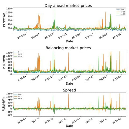
Figure 1.
Day-ahead prices, balancing prices, and spread for sample hours, , quoted on each day from the period from 1 January 2016 until 1 January 2018.
3. Construction of a Selling Strategy
3.1. The Model
ARX is a common model for electricity price forecasting [,,,,,]. It is a linear model, which uses past values of the predicted variables and some time series of exogenous (explanatory) features that are supposed to affect the modeled variable. Here, following [], we assume that:
where:
- is a vector of dummy variables for Monday, Saturday, Sunday/Holidays, and the other days of the week,
- is a vector of exogenous variables,
- L is a set corresponding to a pre-defined lag structure. It means that if , the observation from the day is one of the explanatory variables included in electricity price forecast for day t. In this paper , and are considered,
- and are vectors of coefficients, which correspond to and , respectively,
- is an autoregressive parameter,
- is a coefficient describing the influence of the price from the day-ahead market on the balancing price,
- is independent, identically distributed noise with a finite variance.
The use of the coefficient is motivated by the fact that, when a seller has to make his decision on day not all prices from for the balancing market are already known. Therefore, instead, the prices from the day-ahead market are used.
3.2. Probabilistic Forecasting
We use the ARX model for probabilistic forecasting of electricity price, an approach that has recently gained much interest in energy markets modeling literature (see [] for a review). Definitely, forecasting the whole distribution of the possible next day prices gives more information to the market participants than the point forecast. It can be used not only for the future profits evaluation but also for risk management purposes and optimization of the so called risk–return trade off.
In general, the probabilistic forecast can be defined as “predictive probability distribution over future quantities or events of interest“ []. There are two common approaches in the probabilistic forecast evaluation. In the first one the forecasted random variable is split into the point forecast and the error distribution, i.e., and these two variables are separately estimated. The distribution of can be estimated in many ways. In the paper we apply the historical simulation method (see Section 3.2.1). The second approach is based on finding the distribution of the forecasted random variable itself. This approach will be used in Section 3.2.2 for the Quantile Regression Averaging (QRA) method. Usually, the probabilistic forecasts are used in the form of Prediction Intervals (PIs), being the selected quantiles of the forecasted random variable distribution. Here, however, we use the forecasted distribution for simulations of the possible next day price scenarios.
An analysis of probabilistic forecast requires dividing a dataset into the calibration and validation windows. The calibration window is used for the model estimation. The obtained parameters are then used for the next day, i.e., first day of the validation window and price predictions. Next, the calibration window is moved by one day and the procedure is repeated. The rolling window scheme is applied until predictions for the last day of the validation window are made. Here, the calibration window length is set to 365 days, as in [] it gave the best results for disaggregated, hourly models. Precisely, the predictions are made for each day starting from the second year of the analyzed period (i.e., from 1 January 2017 until 31 January 2018) based on the preceding 365 days. Analogously, the optimization framework is evaluated day-by-day from 1 January 2017 until 31 January 2018.
3.2.1. Historical Simulation
In the historical simulation method various scenarios based on the point forecasts and the historical values of the model residuals are created. We assume that the actual prices and are given by:
where and are the point forecasts of the day-ahead and the balancing prices in day t and hour h, while and are the corresponding residuals. In order to make simulations of the price scenarios from the validation window, the point forecasts of these prices were calculated using the ARX models described by Equations (1) and (2) and combined with the corresponding samples of residuals and . These scenarios can be expressed by:
where . The procedure was applied for different combinations of exogenous variables and lag structures, as described in Table 3.
Table 3.
Results of the proposed strategies based on the maximization of the quantile (maximal profit objective), quantile (minimal risk objective), and quantile (maximal median objective) of portfolio’s forecasted value for different combinations of lags and exogenous variables as well as of the benchmark strategy with the same model structures. The best results for each strategy are marked in bold.
3.2.2. Quantile Regression Averaging
As there is no model structure that significantly outperforms the others, we also use the quantile regression averaging approach which proved to be a good solution in such case. This method is based on the quantile regression model, described by Koenker and Basset in 1978 [] and has been used for probabilistic forecasting of electricity prices in []. The main idea of the method is to determine prediction intervals using a pool of point forecasts obtained from individual models. Prediction intervals are then calculated as a solution of the optimization problem given by []:
where denotes the conditional qth quantile of the distribution of electricity price, are the explanatory variables, being in this case the point predictions of electricity prices and denotes the vector of weights corresponding to the particular predictions from . For a chosen quantile q these weights are estimated by minimizing the loss function:
Here, we extend the quantile regression averaging scheme for a construction of different scenarios of electricity price, described by Equation (7). Using quantile regression models with individual point predictions taken as independent variables we make predictions of particular quantiles of and distributions. Next, having these predictions, we obtain and approximations in . Using the inverse CDF method of a random variable simulation, we construct a set of day-ahead and balancing price scenarios. Recall that a random variable X with cumulative distribution function can be simulated as where U is a uniform random variable on . Note, that from the quantile regression averaging method the values of and are derived only in a given discrete set of points, here in . Hence, the missing values have to be interpolated for randomly generated .
The quantile regression averaging method requires two steps for the forecast derivation. First the individual point forecasts are to be made, second they are used in the quantile regression for the prediction intervals calculation. As a consequence the calibration window has to be divided into two subsets. Here, we use the first 180 data points to calibrate the individual models and next 185 data points for regressing the point forecasts. The validation window is the same as in the historical simulation approach. The algorithm for constructing different scenarios of the day-ahead prices for day t and hour h consists of the following steps:
- Take the predicted values and build quantile regression models fortreating each individual prediction as independent variable.
- On the base of the obtained models, for , make prediction of the qth quantile of distribution and construct its inverse cumulative distribution functions .
- Generate vector of independent, uniform random variables on [0,1].
- For each , with interpolate a single day-ahead price scenario as:
The different scenarios of the balancing prices are constructed using the same procedure.
3.3. Optimization of the Selling Strategy
Now, we focus on the optimization of the electricity selling strategy. To this end, we utilize probabilistic forecast scenarios obtained using methods described in the previous sections. We assume that on day an electricity producer decides on the share of energy sold on the balancing market. The remaining part is sold on the day-ahead (spot) market. The various selling price scenarios can then be constructed as:
where is the share of energy which is sold on the balancing market.
An important issue for the optimal strategy construction is the choice of an optimization criterion. As we want to allow for a trade off between risk and return, we utilize the value at risk notion [], a standard measure in risk management. This is simply a given quantile of the profit/loss distribution. In this context, maximizing the lower quantiles of the selling price, , distribution minimizes the sellers risk. On the other hand, maximizing the upper quantiles maximizes the sellers profit. The risk–return trade off can be achieved by maximizing the middle quantiles of the selling price distribution. Here, we apply all three approaches. Specifically, having a vector , the objective is to find maximum:
where is a quantile of order of conditional distribution under the condition that the share of the electricity on the balancing market is equal to
The process of determining the optimal weights is divided into two parts. In the first part we calculate the selling price scenarios for a discrete set of possible weights . Next, the weight maximizing the selected quantile of the forecasted selling prices is chosen as a starting point in the optimization routine (here we use Python minimization function based on the sequential least squares programming method). The first step of the procedure allows to avoid finding local maximums of the objective function. The optimization procedure have to be repeated for each day t and hour h of the calibration window. It can be summarized in the following way:
- Calculate different values with and .
- For each of calculate .
- Select which maximizes for .
- Apply the sequential least square programming method with taken as a starting point in the maximization of for .
3.4. Strategy Evaluation Metrics
In order to analyze economical benefits from applying the proposed strategy we compare it with the basic and most common practice of selling the whole electricity only on the day-ahead market. Then, the hourly profit can be calculated as:
where is the share of energy sold on the balancing market. In order to compare profitability of different strategies we will use the total profit calculated for all days and hours from the validation window:
where is given by Equation (9). A similar approach was used in []. However, the authors analyzed only the case in which the whole electricity is sold in one of the markets, i.e., with weights being either 1 or 0.
The profit of a possible selling strategy is obviously an important indicator of its usefulness. The second important issue is risk associated with a given strategy. Hence, we also calculate 5% Value at Risk (VaR):
of daily profits , where denotes the empirical cumulative distribution function of . It indicates the level of a potential loss. With this definition, the higher is VaR, the lower is the risk.
4. Results
We apply the proposed optimization of the selling strategy to data from the Polish day-ahead and balancing electricity markets, in details described in Section 2. To this end, we first construct probabilistic forecasts of the balancing electricity price and the day-ahead price . Next, we simulate various scenarios of the selling price, based on the share of electricity sold on the balancing market, . Since there is no model structure that significantly outperforms the others, we use different combinations of the lag structures and the exogenous variables in the ARX model, see Section 3. Finally, we optimize a given economical criterion with respect to the shares . The results of applying the proposed strategy in the validation window are compared with the strategy of [], denoted as the benchmark strategy. Recall that this strategy is based on selling the whole electricity on the market with the higher price point forecast.
4.1. Profit-Maximization Based Strategy
We start with a strategy designed to maximize the selling price, see Equation (4), achieved by an electricity seller. To this end, we find the share of electricity sold on the balancing market, , that maximizes the value of the 0.95 quantile of the constructed portfolios forecasted value. The procedure is repeated (i.e., the decision is made) for each day of the validation window. Assuming that the strategy to sale from 1 MWh of energy on the balancing market and on the day-ahead market would be accepted, the total profit , see Equation (10), and its 5% VaR were calculated. The comparison of the results obtained for the proposed strategy with the results obtained for the benchmark one for different combinations of the exogenous variables and different lag structures is presented in Table 3. We also extend the conducted research with a quantile regression method of scenarios generation, described in Section 3.2.2. Recall that in this method all of the considered point forecast models are combined.
Table 3 indicates that for each of the compared combinations of the lag structures and exogenous variables the total profit obtained with the proposed strategy was higher than the total profit obtained with the benchmark strategy based on the same exogenous variables and lag structures. In each of the considered cases the increase of profit is, however, connected with the increase of the risk, what is indicated by the value of the 5% VaR. In all of the considered cases it is related to the significant increase in the share of sales on the balancing market, which in daily terms is illustrated in Figure 2.
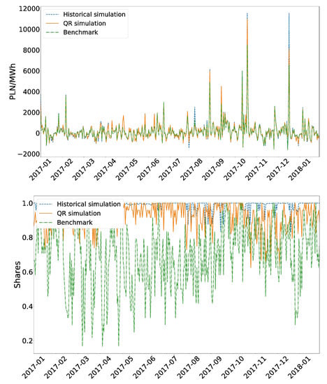
Figure 2.
Daily profits from the benchmark strategy and the strategy based on maximization of the quantile of the future portfolios value (top panel). Daily shares of sale on the balancing market associated with the benchmark strategy and the proposed quantiles maximization strategy (bottom panel). The results of the historical method are plotted for the model structure yielding the highest profit, i.e., with , , and .
Profits obtained with the proposed strategy are rather similar among the considered sets of exogenous variables and lag structure. However, it is worth to notice, that the set of parameters which has brought the highest profit for the proposed strategy, i.e., and with , for the benchmark strategy is not the most profitable. Looking at the results of the QRA method, we can notice that the total profit is in this case lower than for any of the model structures of the historical method, but still it is significantly higher that all of the profits obtained for the benchmark strategy. On the other hand, the risk associated with the strategy based on QRA is lower than the risk obtained with the historical simulation method. Still it is higher, than the risk of the benchmark strategy. Hence, in this case QRA can be regarded as a method compromising increase of the profit with lowering the risk.
4.2. Risk-Minimization Based Strategy
Since the investors not only look on the expected gain, but also on the minimization of the risk associated with the chosen strategy, another approach has also been considered. The risk minimization strategy is based on the maximization of the value at risk—A standard risk measure. Using the simulated selling price scenarios, the value of 0.05 quantile of the constructed portfolios distribution was maximized with respect to the share of electricity sold on the balancing market. It allowed to cut off the most risky scenarios. Again, for the chosen strategy, the total profit and its VaR were calculated. The obtained results are given in Table 3.
As we can see, the goal of reducing the risk associated with selling electricity has been achieved. The VaR of daily profits is significantly higher than in the case of the benchmark strategy, but at the same time, the total profit is much lower. This is due to the fact that the maximization of quantile leads to a strategy that largely focuses on selling on the day-ahead market. The share of sales on the balancing market in daily terms, for both of the strategies, is presented in Figure 3. The strategy obtained with the QRA method yields higher profit than most of the model structures (besides ) with risk being at the similar level. It is interesting to note, that using the risk-minimization strategy the obtained VaR is close to zero, with profits much larger than zero. It means that severe losses are very uncommon, while an extra profit can be achieved. This is illustrated by the top panel of Figure 3. The obtained profit in daily terms is usually smaller than of the benchmark strategy, but at the same time daily losses are also much lower.
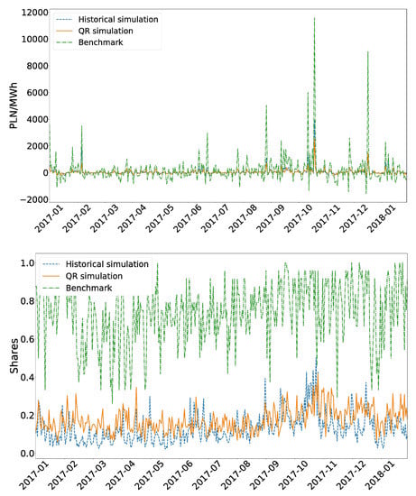
Figure 3.
Daily profits from the benchmark strategy and the strategy based on maximization of the quantile of the future portfolios value (top panel). Daily shares of sale on the balancing market associated with the benchmark strategy and the proposed quantiles maximization strategy (bottom panel). The results of the historical method are plotted for the model structure yielding the minimal risk, i.e., with , , , and .
4.3. Median-Maximization Based Strategy
Finally, we analyze results obtained by maximizing the median of the forecasted selling price distribution, rather than its tails, focusing on moderate scenarios. The results presented in Table 3 indicate that in each of the considered combinations of lag structures and exogenous variables, the obtained total profit was lower when we have applied the proposed strategy with historical simulation method, but in most cases it was also connected with the decrease of risk associated with selling electricity on the balancing market. Again, the optimal model structures are different for the proposed and the benchmark strategy.
The best results were definitely obtained with the QRA method. The total profit was higher than all of the values obtained with the historical method, being at the same time associated with the lowest risk. Comparing the QRA results with the benchmark strategy, we can see that the risk was in all cases much lower for the proposed strategy. On the other hand, the profit was also higher in most cases, with an exception only for and , and , and finally . It seems that the QRA method, based on the point forecasts averaging, is the best choice for moderate selling scenarios. For the chosen sets of parameters a comparison of daily profits and shares is illustrated in Figure 4.
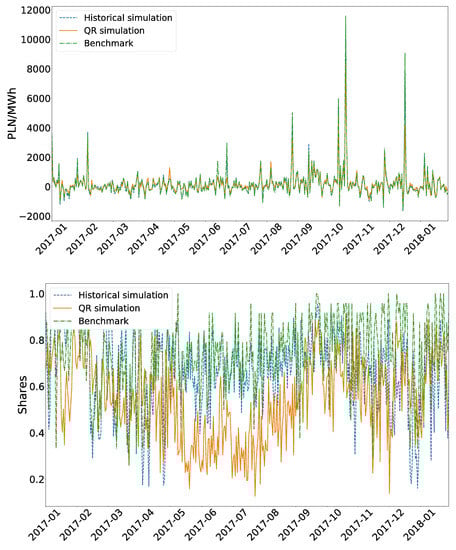
Figure 4.
Daily profits from the benchmark strategy and the strategy based on maximization of the median of the future portfolios value (top panel). Daily shares of sale on the balancing market associated with the benchmark strategy and the proposed medians maximization strategy (bottom panel). The results of the historical method are plotted for the model structure yielding the highest profit, i.e., with , , and .
4.4. Comparison of the Strategies
In Figure 5 we compare daily profits obtained using the profit-maximization, median-maximization, and the risk minimization strategies for the QRA method. Looking on the plot, as expected, daily profits are the highest for the profit-maximization based strategy, whereas they are the lowest for the strategy based on the risk-minimization. At the same time, we can observe the lowest volatility for the risk-minimization strategy and the highest for the profit-maximization. It confirms a well known fact, that higher profits are usually associated with higher risk. The median-maximization strategy profits are between the other two strategies.
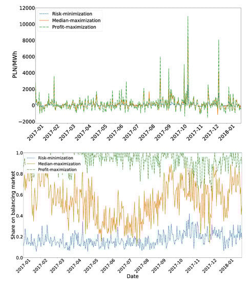
Figure 5.
Daily profits (top panel) and daily shares of sale on the balancing market (bottom panel) for the considered strategies constructed using the Quantile Regression Averaging (QRA) method.
An interesting picture can be observed on the plot of daily shares of sale in the balancing market, which are presented in the bottom panel of Figure 5. The risk-minimization strategy involves most trade in the less volatile and at the same time more safe day-ahead market. However, the optimal strategy still requires selling of about of electricity on the balancing market and there is none day for which the whole electricity should be sold on the day-ahead market. For the profit-maximization strategy the situation is opposite. If an electricity producer is focused on making a maximal possible profit, he should sell most of electricity on the balancing market, with a mean share of about . There are days in which the whole electricity should be sold on the balancing market according to this strategy. Again, for the median-maximization strategy the share of sales on the balancing market is in most days between the other two strategies, with a mean daily share of about .
5. Conclusions
Looking from a perspective of an electricity seller, an optimization of a selling strategy can be based on different factors. Both, the profit maximization and the risk minimization can be the target of the optimization. Although this subject is still a current and important problem, there is only little literature on this topic. With this paper we try to fill the gap and propose a novel approach to the optimization of the selling strategy based on probabilistic forecasting of the day-ahead and the balancing prices of energy. For this purpose, two methods of constructing strategies have been proposed, implemented, and compared with the benchmark selling strategy based on point ARX forecasts proposed recently by the authors of [].
With the chosen optimization scheme we can build a strategy that responds to a given objective, e.g., risk minimization or profit maximization. The risk-minimization and the profit-maximization strategies have let us to achieve the objective, but while applying these methods, an increase of profit was associated with a significant increase of risk. In the case of the median-maximization based strategy, which can be interpreted as a strategy utilizing maximization of the middle of the portfolio, the quantile regression averaging method has brought the most satisfactory results. In this case, we have obtained a higher total profit than in any of the cases based on the historical simulation and most cases of the benchmark strategy. At the same time, the risk associated with selling on the balancing market has been decreased.
Although the developed strategy can probably be still refined using other methods of probabilistic forecasting, we believe that the proposed approach can significantly improve a decision making process for electricity sellers. It can be also easily extended to electricity buyers or another markets where a decision on a selling platform is an important issue. It should be noted, however, that in the paper we have considered a truly marginal producer, whose decisions on the supply quantity do not influence the market prices. If the market is large relative to a small individual power plant, like in the case of the day-ahead market, then this influence is negligible. On the other hand, for smaller markets, like the balancing market, a shift on the supply side could have a considerable effect on price. A possible solution for this problem is to analyze the supply and demand curves (see e.g., the recently proposed X model, []), instead of directly forecasting the clearing price.
Author Contributions
Conceptualization, J.J.; data curation, A.M.; formal analysis, J.J. and A.M.; methodology, J.J.; software, A.M.; supervision, J.J.; validation, A.M.; visualization, A.M.; writing—original draft, J.J. and A.M. All authors have read and agreed to the published version of the manuscript.
Funding
This research received no external funding.
Conflicts of Interest
The authors declare no conflict of interest.
References
- Eurostat. Available online: https://ec.europa.eu/eurostat/statistics-explained (accessed on 17 January 2020).
- Gianfreda, A.; Parisio, L.; Pelagatti, M. The impact of RES in the Italian day-ahead and balancing markets. Energy J. 2016, 37, 161–184. [Google Scholar] [CrossRef]
- Martinez-Anido, C.B.; Brinkman, G.; Hodge, B. The impact of wind power on electricity prices. Renew. Energy 2016, 94, 474–487. [Google Scholar] [CrossRef]
- Woo, C.K.; Moore, J.; Schneiderman, B.; Ho, T.; Olson, A.; Alagappan, L.; Chawlab, K.; Toyamad, N.; Zarnikau, J. Merit-order effects of renewable energy and price divergence in California’s day-ahead and real-time electricity markets. Energy Policy 2016, 92, 299–312. [Google Scholar] [CrossRef]
- Uniejewski, B.; Marcjasz, G.; Weron, R. Understanding intraday electricity markets: Variable selection and very short-term price forecasting using LASSO. Int. J. Forecast. 2019, 35, 1533–1547. [Google Scholar] [CrossRef]
- Maciejowska, K.; Nitka, W.; Weron, T. Day-ahead vs. intraday—Forecasting the price spread to maximize economic benefits. Energies 2019, 12, 631. [Google Scholar] [CrossRef]
- Weron, R. Electricity price forecasting: A review of the state-of-the-art with a look into the future. Int. J. Forecast. 2014, 30, 1030–1081. [Google Scholar] [CrossRef]
- Karakatsani, N.V.; Bunn, D.W. Forecasting electricity prices: The impact of fundamentals and time-varying coefficients. Int. J. Forecast. 2008, 24, 764–785. [Google Scholar] [CrossRef]
- Kristiansen, T. Forecasting nord pool day-ahead prices with an autoregressive model. Energy Policy 2012, 49, 328–332. [Google Scholar] [CrossRef]
- Kosater, P.; Mosler, K. Can Markov regime-switching models improve power-price forecasts? Evidence from German daily power prices. Appl. Energy 2006, 83, 943–958. [Google Scholar] [CrossRef]
- Janczura, J.; Weron, R. An empirical comparison of alternate regime-switching models for electricity spot prices. Energy Econ. 2010, 32, 1059–1073. [Google Scholar] [CrossRef]
- Bessa, R.J.; Trindade, A.; Miranda, V. Spatial-temporal solar power forecasting for smart grids. IEEE T. Ind. Inf. 2015, 11, 232–241. [Google Scholar] [CrossRef]
- Corizzo, R.; Pio, G.; Ceci, M.; Malerba, D. DENCAST: Distributed density-based clustering for multi-target regression. J. Big Data 2019, 6, 43. [Google Scholar] [CrossRef]
- Weron, R.; Misiorek, A. Forecasting spot electricity prices: A comparison of parametric and semiparametric time series models. Int. J. Forecast. 2008, 24, 744–763. [Google Scholar] [CrossRef]
- Monteiro, C.; Ramirez-Rosado, I.J.; Fernandez-Jimenez, L.A.; Conde, P. Short-term price forecasting models based on artificial neutral networks for intraday sessions in the Iberian electricity markets. Energies 2016, 9, 721. [Google Scholar] [CrossRef]
- Ceci, M.; Corizzo, R.; Malerba, D.; Rashkovska, A. Spatial autocorrelation and entropy for renewable energy forecasting. Data Min. Knowl. Disc. 2019, 33, 698. [Google Scholar] [CrossRef]
- Abdel-Nasser, M.; Mahmoud, K. Accurate photovoltaic power forecasting models using deep LSTM-RNN. Neural Comput. Appl. 2019, 31, 2727–2740. [Google Scholar] [CrossRef]
- Areekul, P.; Senju, T.; Toyama, H.; Chakraborty, S.; Yona, A.; Urasaki, N.; Mandal, P.; Saber, A.Y. New method for next-day price forecasting for PJM electricity market. Int. J. Emerg. Electr. Power Syst. 2010, 11, 3. [Google Scholar] [CrossRef]
- Narajewski, M.; Ziel, F. Econometric modelling and forecasting of intraday electricity prices. J. Commod. Mark. 2019. [Google Scholar] [CrossRef]
- Poplawski, T.; Dudek, G.; Łyp, J. Forecasting methods for balancing energy market in Poland. Int. J. Electr. Power 2015, 65, 94–101. [Google Scholar] [CrossRef]
- Kiesel, R.; Paraschiv, F. Econometric analysis of 15-minute intraday electricity prices. Energy Econ. 2017, 64, 77–90. [Google Scholar] [CrossRef]
- Ortner, A.; Totschnig, G. The future relevance of electricity balancing markets in Europe—A 2030 case study. Energy Strateg. Rev. 2019, 24, 111–120. [Google Scholar] [CrossRef]
- Nowotarski, J.; Weron, R. Recent advances in electricity price forecasting: A review of probabilistic forecasting. Renew. Sust. Energ. Rev. 2018, 81, 1548–1568. [Google Scholar] [CrossRef]
- Andrade, J.R.; Filipe, J.; Reis, M.; Bessa, R.J. Probabilistic price forecasting for day-ahead and intraday markets: Beyond the statistical model. Sustainability 2017, 9, 1990. [Google Scholar] [CrossRef]
- Browell, J. Risk constrained trading strategies for stochastic generation with a single-price balancing market. Energies 2018, 11, 1345. [Google Scholar] [CrossRef]
- TGE. Available online: https://tge.pl/statistic-data (accessed on 17 February 2020).
- PSE. Available online: https://www.pse.pl/web/pse-eng/data (accessed on 17 February 2020).
- Hubicka, K.; Marcjasz, G.; Weron, R. A note on averaging day-ahead electricity price forecasts across calibration windows. IEEE T. Sustain. Energ. 2019, 10, 321–323. [Google Scholar] [CrossRef]
- Maciejowska, K.; Nowotarski, J.; Weron, R. Probabilistic forecasting of electricity spot prices using factor quantile regression averaging. Int. J. Forecast. 2016, 32, 957–965. [Google Scholar] [CrossRef]
- Marcjasz, G.; Serafin, T.; Weron, R. Selection of calibration windows for day-ahead electricity price forecasting. Energies 2018, 11, 2364. [Google Scholar] [CrossRef]
- Gneiting, T.; Katzfuss, M. Probabilistic forecasting. Annu. Rev. Stat. Appl. 2014, 1, 125–151. [Google Scholar] [CrossRef]
- Koenker, R.; Basset, G. Regression quantiles. Econometrica 1978, 46, 33–50. [Google Scholar] [CrossRef]
- Nowotarski, J.; Weron, R. Computing electricity spot price prediction intervals using quantile regression and forecast averaging. Comput. Stat. 2015, 30, 791–803. [Google Scholar] [CrossRef]
- McNeil, A.J.; Frey, R.; Embrechts, P. Quantitative Risk Management: Concepts, Techniques and Tools: Concepts, Techniques and Tools; Princeton University Press: Princeton, NJ, USA, 2005; p. 38. [Google Scholar]
- Ziel, F.; Steinert, R. Electricity price forecasting using sale and purchase curves: The X-Model. Energy Econ. 2016, 59, 435–454. [Google Scholar] [CrossRef]
© 2020 by the authors. Licensee MDPI, Basel, Switzerland. This article is an open access article distributed under the terms and conditions of the Creative Commons Attribution (CC BY) license (http://creativecommons.org/licenses/by/4.0/).