Sequence Impedances of Land Single-Core Insulated Cables: Direct Formulae and Multiconductor Cell Analyses Compared with Measurements


Abstract
:
1. Introduction
- Different lengths in the minor sections provoke not zeroed induced currents in the screens;
- Joint chambers and terminals which force a flat arrangement with a consequent asymmetry;
- The crossings of interfering services or natural obstacles, if any, usually overcome by directional drillings which may introduce a great cable spacing;
- That the as-built installation is always different from the project.
2. Normative and Council Direct Formulae for Computing Cable Sequence Impedances
3. MCA for Evaluating Sequence Impedances of Cable Systems
4. Description of the Four Reference Cable Systems
5. Measurement Campaigns
6. IEC/Cigré Computations
7. Some Notes on MCA Results
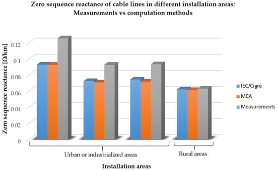
8. Final Comparisons of MCA and IEC/Cigrè with Measurements
- RED for errors greater than 15 %;
- YELLOW for errors ranging between 7.5% and 15%;
- GREEN for errors smaller than 7.5%.
9. Conclusions
- (1)
- The minor section lengths are exactly equal (practically impossible);
- (2)
- There is perfect laying symmetry along the route (trefoil laying or any laying performed with phase transpositions: both very difficult to obtain).
Author Contributions
Funding
Conflicts of Interest
References
- Benato, R.; Caciolli, L. Sequence impedances of insulated cables: Measurements versus computations. PES T&D 2012, 2012, 1–7. [Google Scholar] [CrossRef]
- IEC 60909-2: Short-Circuit Currents in Three-Phase a.c. Systems—Part 2: Data of Electrical Equipment for Short-Circuit Current Calculations, 2nd ed.; IEC: Geneva, Switzerland, 2008.
- Royer, C.; Dorison, E.; Anderson, N.; Benato, R.; Brijs, B.; Chang, K.W.; Falconer, A.; Fernandez, S.; Gudmunsdottir, U.S.; Li, J.; et al. Cable Systems Electrical Characteristics. Technical Report for CIGRE Technical Brochure N°531. 2013. Available online: https://e-cigre.org/publication/531-cable-systems-electrical-characteristics (accessed on 28 February 2020).
- Ametani, A.; Ohno, T. Derivation of Theoretical Formulas of Sequence Currents on Underground Cable Systems. IEEJ Trans. Power Energy 2011, 131, 277–282. [Google Scholar] [CrossRef]
- Ramya, G.M.; Radhika, P. Computation of Sequence Impedances for 220kv Underground Cable with Different Short Circuit Capacities. Int. J. Mod. Trends Sci. Technol. 2017, 3. Available online: http://www.ijmtst.com (accessed on 28 February 2020).
- Benato, R. Multiconductor analysis of underground power transmission systems: EHV AC cables. Electr. Power Syst. Res. 2009, 79, 27–38. [Google Scholar] [CrossRef]
- Benato, R.; Paolucci, A. Multiconductor cell analysis of skin effect in Milliken type cables. Electr. Power Syst. Res. 2012, 90, 99–106. [Google Scholar] [CrossRef]
- Benato, R.; Napolitano, D. Overall Cost Comparison between Cable and Overhead Lines Including the Costs for Repair After Random Failures. IEEE Trans. Power Deliv. 2012, 27, 1213–1222. [Google Scholar] [CrossRef]
- Benato, S.R.; Dambone Sessa, F.; Guglielmi, E.; Partal, E.; Tleis, N. Ground Return Current Behaviour in High Voltage Alternating Current Insulated Cables. Energies 2014, 7, 8116–8131. [Google Scholar] [CrossRef] [Green Version]
- Benato, R.; Sessa, S.D.; De Zan, R.; Guarniere, M.; Lavecchia, G.; Labini, P.S. Different Bonding Types of Scilla-Villafranca (Sicily-Calabria) 43 km Double-Circuit AC 380 kV Submarine-Land Cable. IEEE Trans. Ind. Appl. 2015, 51, 5050–5057. [Google Scholar] [CrossRef]
- Benato, R.; Colla, L.; Sessa, S.D.; Marelli, M. Review of high current rating insulated cable solutions. Electr. Power Syst. Res. 2016, 133, 36–41. [Google Scholar] [CrossRef]
- Benato, R.; Sessa, S.D.; Guglielmi, F.; Partal, E.; Tleis, N. Zero sequence behaviour of a double-circuit overhead line. Electr. Power Syst. Res. 2014, 116, 419–426. [Google Scholar] [CrossRef]
- Benato, R.; Sessa, S.D.; Guizzo, L.; Rebolini, M. The synergy of the future: high voltage insulated power cables and railway-highway infrastructures. IET Gener. Transm. Distrib. 2017, 11, 2712–2720. [Google Scholar] [CrossRef]
- Benato, R.; Sessa, S.D. A New Multiconductor Cell Three-Dimension Matrix-Based Analysis Applied to a Three-Core Armoured Cable. IEEE Trans. Power Deliv. 2018, 33, 1636–1646. [Google Scholar] [CrossRef]
- Carson, J.R. Wave Propagation in Overhead Wires with Ground Return. Bell Syst. Tech. J. 1926, 5, 539–554. [Google Scholar] [CrossRef]
- Pollaczek, F. Über das Feld einer unendlich langen wechsel stromdurchflossenen Einfachleitung. Electrishe Nachrichten Technik 1926, 3, 339–360. [Google Scholar]
- CCITT. Directives Concerning the Protection of Telecommunication Lines against Harmful Effects from Electric Power and Electrified Railway Lines; CCITT: Geneva, Switzerland, 1989. [Google Scholar]
- Schelkunhoff, S.A. The electromagnetic theory of coaxial transmission lines and cylindrical shields. Bell Syst. Tech. J. 1934, 13, 532–579. [Google Scholar] [CrossRef]
- Wedepohl, L.M.; Wilcox, D.J. Transient analysis of underground power transmission systems. Proc. IEEE 1973, 120, 253–260. [Google Scholar]
- Benato, R.; Sessa, S.D.; Forzan, M. Experimental Validation of 3-Dimension Multiconductor Cell Analysis by a 30 km Long Submarine Three-Core Armoured Cable. IEEE Trans. Power Deliv. 2018, 33, 2910–2919. [Google Scholar] [CrossRef]
- Choi, J.K.; Kwak, J.S.; Lee, W.K.; Jung, C.K.; Kim, J.W.; Oh, S.I. Analysis of Sequence impedance of 345 kV Cable systems with Special bondings using ATP. In Proceedings of the 2009 Transmission & Distribution Conference & Exposition: Asia and Pacific, Seoul, South Korea, 26–30 October 2009. [Google Scholar]
- Gudmundsdottir, U.S.; Gustavsen, B.; Bak, C.L.; Wiechowski, W. Field Test and Simulation of a 400-kV Cross-Bonded Cable System. IEEE Trans. Power Deliv. 2011, 26, 1403–1410. [Google Scholar] [CrossRef]
- Das, J.C. Understanding Symmetrical Components for Power System Modelling; IEEE Press Wiley: Hoboken, NJ, USA, 2017. [Google Scholar]
- Tleis, N. Power Systems Modelling and Fault Analysis: Theory and Practice, 2nd ed.; Newnes: London, UK, 2019. [Google Scholar]
- Blackburn, J.L. Symmetrical Components for Power Systems Engineering; CRC Press: Boca Raton, FL, USA, 1993. [Google Scholar]
- IEC 60909-3: Short-Circuit Currents in Three-Phase a.c. Systems—Part 3: Currents during Two Separate Simultaneous Line-to-Earth Short-Circuits and Partial Short-Circuit Currents Flowing through Earth; IEC: Geneva, Switzerland, 2010.
- IEC EN 60044-1, Instrument Transformers—Part 1: Current Transformers; IEC: Geneva, Switzerland, 1999.
- IEC EN 60044-5, Instrument Transformers—Part 5: Capacitor Voltage Transformers; IEC: Geneva, Switzerland, 2004.
- Callegaro, L. Electrical Impedance Principles, Measurement, and Applications; Taylor & Francis Group: Milton Park, UK, 2013. [Google Scholar]
- IEC 60287: Electric Cables—Calculation of the Current Rating, (in 8 parts: 1.1, 1.2, 1.3, 2.1, 2.2, 3.1, 3.2, 3.3); IEC: Geneva, Switzerland, 2015.


| Line Geometrical Characteristics | ||
| Total length | km | 8.325 |
| Trefoil laying length | km | 6.495 |
| Flat laying (spacing =1 m) length | km | 1.785 |
| Trefoil in ducts length (duct spacing = 0.150 m) | km | 0.045 |
| Conductor cross section and material | mm2 | 1000 Al |
| Screen Arrangement | cross-bonding | |
| Conductor diam. (dc) | mm | 38.4 |
| Conductor semic. screen diameter (d0) | mm | 42.3 |
| Insulating material diameter (d1) | mm | 83.1 |
| Insulating semic. screen diam. | mm | 85.3 |
| Metallic screen diameter | mm | 87.5 |
| Screen cross-section | mm2 | 85 |
| External jacket diameter | mm | 96 |
| Line Geometrical Characteristics | ||
| Total length | km | 5.868 |
| Trefoil laying length | km | 4.743 |
| Open trefoil length (spacing = 0.225 m) | km | 0.886 |
| Flat laying (spacing = 0.35 m) length | km | 0.239 |
| Conductor cross section and material | mm2 | 1600 Al |
| Screen Arrangement | cross-bonding | |
| Conductor diameter (dc) | mm | 47.5 |
| Conductor semic. screen diameter (d0) | mm | 52.9 |
| Insulating material diameter (d1) | mm | 86.9 |
| Insulating semic. screen diam. | mm | 90.7 |
| Equivalent metallic screen diameter | mm | 91.93 |
| Copper screen cross-section | mm2 | 140 |
| Aluminium screen cross-section | mm2 | 60 |
| External jacket diameter | mm | 106 |
| Line Geometrical Characteristics | ||
| Total length | km | 10.851 |
| Trefoil laying length | km | 9.831 |
| Flat laying (spacing = 0.25 m) length | km | 0.204 |
| Trefoil in ducts length (duct spacing = 0.180 m) | km | 0.267 |
| FlowMole (guide drill system) length (spacing = 0.5 m) | km | 0.549 |
| Conductor cross section and material | mm2 | 1600 Al |
| Screen Arrangement | cross-bonding | |
| Conductor diameter (dc) | mm | 49.1 |
| Conductor semic. screen diameter (d0) | mm | 51.1 |
| Insulating material diameter (d1) | mm | 89.1 |
| Insulating semic. screen diam. | mm | 93.1 |
| Copper screen inner diameter | mm | 93.9 |
| Copper screen cross-section | mm2 | 70 |
| Copper screen thickness | mm | 1.35 |
| Aluminium foil inner diameter | mm | 97.4 |
| Aluminium foil cross-section | mm2 | 61.3 |
| Aluminium foil thickness | mm | 0.2 |
| External jacket diameter | mm | 105.8 |
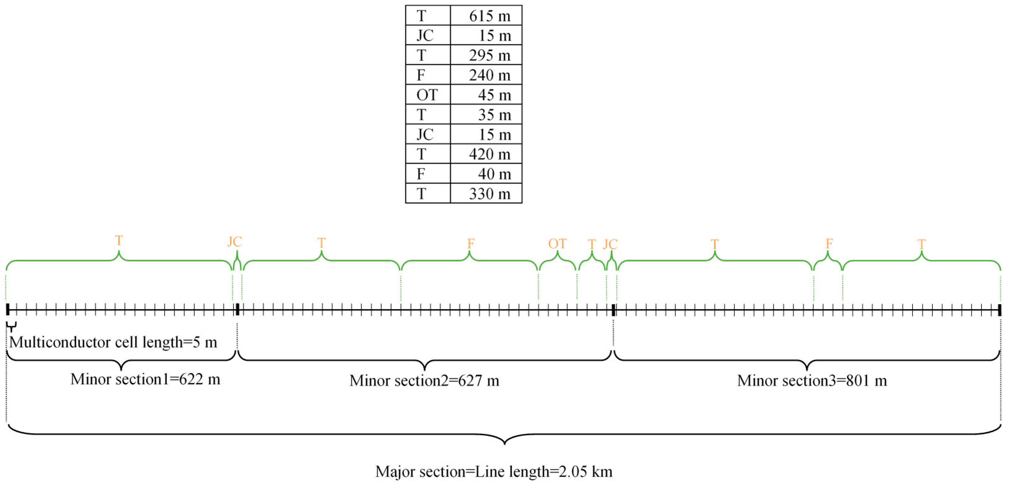
| Line Geometrical Characteristics | ||
| Total length | km | 2.05 |
| Trefoil laying length | km | 1.695 |
| Open trefoil laying length (spacing = 0.20 m) | km | 0.045 |
| Flat laying (spacing = 0.60 m) length | km | 0.310 |
| Conductor cross section and material | mm2 | 1600 Cu |
| Screen Arrangement | cross-bonding | |
| Conductor diameter (dc) | mm | 49.4 |
| Conductor semic. screen diameter (d0) | mm | 53.8 |
| Insulating material diameter (d1) | mm | 107.8 |
| Insulating semic. screen diameter | mm | 110.8 |
| Equivalent metallic screen diameter | mm | 115.3 |
| Copper screen cross-section | mm2 | 122 |
| Lead screen outer diameter | mm | 121.8 |
| Lead screen cross-section | mm2 | 748 |
| External jacket diameter | mm | 132 |
| Electrical Quantity | #1 1000 Al | #2 1600 Al | #3 1600 Al | #4 2500 Cu |
|---|---|---|---|---|
| DC p.u.l. conductor resistance at 20 °C in Ω/km | 0.0291 | 0.0186 | 0.0186 | 0.0113 |
| AC p.u.l. conductor resistance at 20 °C in Ω/km | 0.0323 | 0.0227 | 0.0224 | 0.0162 |
| Screen or equiv. screen p.u.l. resistance at 20 °C in Ω/km | 0.216 | 0.0977 | 0.162 | 0.0946 |
| Relative permittivity of insul. | 2.7 | 2.5 | 2.3 | 2.3 |
| Case #1 | Case #2 | Case #3 | Case #4 | |
|---|---|---|---|---|
| Shunt capacitance c | 0.22 | 0.2755 | 0.2320 | 0.1889 |
| Sequence Impedances | Z1= R1+ jX1 | Z0= R0+ jX0 |
|---|---|---|
| Case #1 | 0.3074 + j1.2548 | 1.9549 + j1.0452 |
| Case #2 | 0.1588 + j0.7623 | 0.6832 + j0.3699 |
| Case #3 | 0.2685 + j1.3882 | 2.0252 + j1.0054 |
| Case #4 | 0.0479 + j0.2864 | 0.2435 + j0.1913 |
| Phase Number | 1 | 2 | 3 |
|---|---|---|---|
| Phase voltage magnitudes V | 52.27 | 52.03 | 52.05 |
| Phase current magnitudes A | 40.51 | 39.91 | 40.61 |
| Phase current angles ° | 76.5 | 76.1 | 76.1 |
| Screen current magnitudes A | 1.30 | 1.70 | 1.40 |
| Case #1 | Case #2 | Case #3 | Case #4 | |
|---|---|---|---|---|
| Shunt capacitance c | 0.2225 | 0.2802 | 0.2301 | 0.1842 |
| Sequence Impedances | Z1= R1+ jX1 | Z0= R0+ jX0 |
|---|---|---|
| Case #1 | 0.2821 + j1.2626 | 2.0243 + j0.7733 |
| Case #2 | 0.1405 + j0.7070 | 0.7101 + j0.3634 |
| Case #3 | 0.2627 + j1.2509 | 1.9925 + j0.7874 |
| Case #4 | (0.0311 – 0.035) + j0.2832 | (0.2235 – 0.2274) + j0.1523 |
| Case #1 | Case #2 | Case #3 | Case #4 | |
|---|---|---|---|---|
| Shunt p.u.l. capacitance c | 0.2225 | 0.2802 | 0.2301 | 0.1842 |
| Sequence Impedances | Z1= R1+ jX1 | Z0= R0+ jX0 |
|---|---|---|
| Case #1 | 0.3064 + j1.2446 | 2.1911 + j0.819 |
| Case #2 | 0.1558 + j0.7027 | 0.7256 + j0.3587 |
| Case #3 | 0.2767 + j1.3694 | 1.9991 + j0.7672 |
| Case #4 | (0.0432 – 0.0451) + j0.277 | (0.2807 – 0.2827) + j0.1518 |
| COMPARISON BETWEEN THE DIFFERENT METHODS APPLIED TO THE ANALYSED CASE STUDIES | |||||||||||||
|---|---|---|---|---|---|---|---|---|---|---|---|---|---|
| Case #1 SE Calenzano-SE Rifredi RT | Case #2 CP S. Giuseppe-CP Portoferraio | Case #3 SE Camin-CP Bassanello | Case #4 CP Ferrara Nord-C.le SEF | ||||||||||
| IEC Cigré | MCA | Mea. | IEC Cigré | MCA | Mea. | IEC Cigré | MCA | Mea. | IEC Cigré | MCA | Mea. | ||
| c | μF/km | 0.2224 | 0.2224 | 0.2200 | 0.2802 | 0.2802 | 0.2755 | 0.2301 | 0.2301 | 0.2320 | 0.1842 | 0.1842 | 0.1889 |
| Δe | % | −1.09 | −1.09 | −1.71 | −1.71 | 0.82 | 0.82 | 2.49 | 2.49 | ||||
| R1 | Ω | 0.2821 | 0.3064 | 0.3074 | 0.1405 | 0.1558 | 0.1588 | 0.2627 | 0.2767 | 0.2865 | 0.0311 ÷ 0.0350 | 0.0432 ÷ 0.0451 | 0.0479 |
| Δe | % | 8.23 | 0.33 | 11.52 | 1.89 | 8.31 | 3.42 | 35 ÷ 26.9 | 9.3 ÷ 5.9 | ||||
| X1 | Ω | 1.2626 | 1.2446 | 1.2548 | 0.7069 | 0.7063 | 0.7623 | 1.2509 | 1.3694 | 1.3882 | 0.2832 | 0.2769 | 0.2864 |
| Δe | % | −0.62 | 0.81 | 7.27 | 7.35 | 9.89 | 1.35 | 1.12 | 3.32 | ||||
| R0 | Ω | 2.0243 | 2.0239 | 1.9549 | 0.7101 | 0.7256 | 0.6832 | 1.9925 | 1.9991 | 2.0252 | 0.2235 ÷ 0.2274 | 0.2406 ÷ 0.2434 | 0.2435 |
| Δe | % | −3.55 | −3.53 | −3.94 | −6.21 | 1.61 | 1.29 | 8.2 ÷ 6.6 | −1.19 ÷ −0.04 | ||||
| X0 | Ω | 0.7733 | 0.7711 | 1.0452 | 0.3634 | 0.3587 | 0.3699 | 0.7847 | 0.7672 | 1.0054 | 0.1523 | 0.1470 | 0.1913 |
| Δe | % | 26.01 | 26.22 | 1.76 | 3.03 | 21.95 | 23.69 | 20.39 | 23.16 | ||||
© 2020 by the authors. Licensee MDPI, Basel, Switzerland. This article is an open access article distributed under the terms and conditions of the Creative Commons Attribution (CC BY) license (http://creativecommons.org/licenses/by/4.0/).
Share and Cite
Benato, R.; Dambone Sessa, S.; Poli, M.; Sanniti, F. Sequence Impedances of Land Single-Core Insulated Cables: Direct Formulae and Multiconductor Cell Analyses Compared with Measurements. Energies 2020, 13, 1084. https://doi.org/10.3390/en13051084
Benato R, Dambone Sessa S, Poli M, Sanniti F. Sequence Impedances of Land Single-Core Insulated Cables: Direct Formulae and Multiconductor Cell Analyses Compared with Measurements. Energies. 2020; 13(5):1084. https://doi.org/10.3390/en13051084
Chicago/Turabian StyleBenato, Roberto, Sebastian Dambone Sessa, Michele Poli, and Francesco Sanniti. 2020. "Sequence Impedances of Land Single-Core Insulated Cables: Direct Formulae and Multiconductor Cell Analyses Compared with Measurements" Energies 13, no. 5: 1084. https://doi.org/10.3390/en13051084