Comparing Power-System and User-Oriented Battery Electric Vehicle Charging Representation and Its Implications on Energy System Modeling

Abstract

Battery electric vehicles (BEV) provide an opportunity to balance supply and demand in future power systems with high shares of fluctuating renewable energy. Compared to other storage systems such as pumped-storage hydroelectricity, electric vehicle energy demand is highly dependent on charging and connection choices of vehicle users. We present a model framework of a utility-based stock and flow model, a utility-based microsimulation of charging decisions, and an energy system model including respective interfaces to assess how the representation of battery electric vehicle charging affects energy system optimization results. We then apply the framework to a scenario study for controlled charging of nine million electric vehicles in Germany in 2030. Assuming a respective fleet power demand of 27 TWh, we analyze the difference between power-system-based and vehicle user-based charging decisions in two respective scenarios. Our results show that taking into account vehicle users’ charging and connection decisions significantly decreases the load shifting potential of controlled charging. The analysis of marginal values of equations and variables of the optimization problem yields valuable insights on the importance of specific constraints and optimization variables. Assumptions on fleet battery availability and a detailed representation of fast charging are found to have a strong impact on wind curtailment, renewable energy feed-in, and required gas power plant flexibility. A representation of fleet connection to the grid in high temporal detail is less important. Peak load can be reduced by 5% and 3% in both scenarios, respectively. Shifted load is robust across sensitivity analyses while other model results such as curtailment are more sensitive to factors such as underlying data years. Analyzing the importance of increased BEV fleet battery availability for power systems with different weather and electricity demand characteristics should be further scrutinized.

1. Introduction

1.1. Motivation

The Paris Agreement calls for a nearly carbon-neutral global energy and transport system by 2050 [1]. Furthermore, the European Commission announced that Europe will be climate-neutral by 2050 [2]. In Germany, the transformation of the power system is well underway; however, the transition to a greenhouse gas (GHG) emission free transport system is far behind [3]. In order to achieve transport GHG emission goals, electric vehicles (EVs) are seen as a potential solution when combined with renewable energy sources (RES) [4]. This in turn requires a new integration of the energy and transport sectors.

Integrating the energy and transport sectors requires an alignment of power demand from EVs and power supply from fluctuating RES. In order to address this challenge, increasing flexibility of the power system is necessary to ensure demand is always met [5]. Measures to increase power system flexibility include an expansion of battery storage and sector coupling [6]. Sector coupling allows for the shifting of energy from different sectors such as heating or transport. Designing sector coupling requires a detailed analysis of the interactions and dependencies between the sectors.

Sector coupling in general and EVs in particular will create an additional load on the power system. At the same time, EVs often contain oversized batteries and offer an option for added flexibility in the energy system, assuming they can flexibly charge in contrast to uncontrolled charging [7] (p. 4). Daily demand patterns depend on individual transport demand, charging behavior, infrastructure availability, and differences between working day and weekend travel. Consequently, charging behavior will influence EVs’ role in the electricity system. This serves as the motivation for developing an integrated user behavior focused modeling approach for the interactions between future EV fleets and the energy system.

1.2. Literature Review

In this section, we present a selection of literature related to the potential of integrating EVs in power systems within energy system optimization modeling and more transport related research assessing driving factors for demand patterns, charging dynamics, users’ acceptance for controlled charging, and connection choices of EV users.

Integrating endogenous vehicle market development modeling into energy system modeling has been demonstrated by [8] for the case of the COCHIN-TIMES model for different drive-train technologies.

Transportation research has carried out various research to better understand EV charging related phenomena. The acceptance of utility controlled charging and its respective factors have been assessed for 1470 plug-in EV buyers in Canada [9]. The authors find general acceptance for utility controlled charging among one-half to two-thirds of the respondents interested in buying a plug-in hybrid electric vehicle. Turning more to transportation demand-oriented driving factors for EV charging, Sun et al. show that state-of-charge (SOC), interval in days before the next trip, and vehicle-kilometers to be traveled on the next day are the main predictors for deciding to charge or not [10]. Fischer et al. complement this finding by also mentioning location and comfortable range as determinants of recharge decisions and charging characteristics [7].

Another strand of studies examines the build-up of EV charging infrastructure. Gnann et al. utilized empirical charging data in a queuing model to estimate future fast charging infrastructure requirements [11]. Chakraborty et al. examine the influence of electricity costs on charging behavior and thereby on infrastructure needs [12]. Tian et al. similarly use analysis of charging behavior to optimize the location of charging stations in China [13]. As a final example, Hardman et al. conduct a review of charging preferences in relation to the build-up charging infrastructure [14]. Thus the main focus of charging behavior models and investigations has been on determining charging infrastructure to support the uptake of EVs.

Steck et al. simulate charging behavior of EV users to determine potential emission reductions from shifting charging events [15]. Taking into account user preferences and user specific alternatives, their results show that charging demand can be shifted away from demand peaks due to the price sensitivity of EV users. Schuller shows the impact of controlled charging on RES utilization for EVs. He describes a concentrating effect of charging events when decisions are taken based on power prices [16].

Energy system modeling has been incorporating partly flexible electricity demand by EVs in their models for some time. Brown et al. (2018) describe an over proportionally high increase in system cost with uncontrollable electricity demand from the transport sector. Controlling charging times of battery electric vehicles (BEVs) is described to provide a PV-integrating effect, reducing total system cost by 10% when 25% of the fleet is flexible for a study of the European power system with 95% GHG reduction targets for 2030 [4].

Michaelis et al. assess the role of controlled charging for the German power system in 2030 utilizing the models ALADIN and eLoad taking into account commercial and public charging stations. They reproduce the finding of Schuller et al. (2013) that price-based charging leads to a load concentration around noon in summer and a night and a day peak in winter. They find a 1.8 TWh reduction of RES curtailment and up to 2.2 GW reduction of peak load by controlled charging [17]. However, charging power is limited to a conservative value of 3.7 kW per vehicle. Furthermore, the power system setup is not described so results are hard to compare and the authors call for an assessment of different flexibility options.

Luca de Tena & Pregger assume an additional power demand of 49 TWh/a for EVs in Germany for 2050. In their analysis, system losses are reduced by 1.4 TWh/a in 2030 in the base scenario. Residual peak demand can be reduced by 1.2 GW in 2030 [18].

Gerhardt et al. assume German transport sector’s power demand in 2050 amounting to approximately 120 TWh including light duty vehicles. They assume the vehicle fleet is comprised of 20% BEVs and 40% plug-in hybrid and range extended EVs. RES curtailment is reduced from 12.2 TWh to 10.7 TWh [19].

Taljegaard et al. assess implications of future BEV fleets on power system investments up to 2050 and on power system operation in 2030 for a geographical scope of Scandinavia and Germany. They find that the increase in needed power plant capacities for fulfilling increased electricity demand for the BEV fleet is lower than the increase in annual power demand through increased utilization rates of wind power (2–4%), thermal power plants, and grid interconnectors (increase of 10%), at the same time implying decreased cycling of thermal power plants. Furthermore, a potential EV fleet may decrease necessary peak power capacity by 13–15 GW by smoothing the net load curve reducing peak net load by 7 GW from 120 to 113 GW. Investments for solar power are drastically reduced by 22–42% due to PV feed-in competing with vehicle-to-grid feed-in in midday peak hours. Taking into account only the optimization of charging hours without feeding back to the grid, electricity costs from operation lies in the same order of electricity costs without optimization with slightly lower costs for an assumed 60% BEV fleet and slightly higher costs for a 100% BEV fleet [20].

Both strands of research, energy system analysis and transport research, provide valuable insights. However, the research fields of energy system analysis and transport research have been carried out in a fairly distinct manner, formulating the interest of each field’s research to the other. So far, this gap has not been bridged to integrate BEV users’ preferences in energy system analytical frameworks. At the same time, energy system model studies are hard to compare since model experiments cannot be reproduced, model scopes vary among the studies and energy system model sensitivities to different aspects of BEV charging has not been assessed in-depth.

Robinius et al. formalize the concept of sector coupling [6] and the challenge of describing different parts of both power and transport systems in adequate detail. They suggest an open model environment where sector and technology specific calculations are carried out in sub-models and interfaced with each other [21]. This approach is adopted in our paper. We use the two terms ‘energy system’ and ‘power system’—differentiating power plants, stationary storage, grids, and power demand (power system) from power demand in the transportation sector (which is part of the energy system).

This paper contributes to the existing literature by providing a first step towards bridging the gap between detailed transport modeling tools and energy system optimization models. By comparing power-system-based and vehicle user-based charging decisions, we identify the most crucial aspects that deserve high analytical detail when representing EV fleets as a potential load shifting option in power systems with high shares of fluctuating renewable energies.

1.3. Scope of This Work

Despite the fact that the flexibility related to the controlled charging of EVs is regarded as potentially highly relevant to the integration of fluctuating RES power generation, the role of EV user behavior, as well as a detailed modeling of charging infrastructure, has received relatively little attention in energy system modeling literature. We address this gap in the literature by specifically analyzing the limitations of charging flexibility related to individual decisions on when, where, and to what degree vehicles are charged. Furthermore, we evaluate the impact of representing these decisions on energy system optimization models results. By combining four models focused on vehicle buyers’ decision making, BEV charging behavior, and the energy system, we answer the following research question:

How are energy system optimization modeling results affected by representing BEV charging based on a power-system oriented perspective vs. a more user-oriented perspective?

We assess this question with regard to annual energy system results such as annual curtailment, added capacities etc. (Section 3.2.1), cost-optimal charging of EV fleets (Section 3.2.2), show explanatory insights (Section 3.2.3), and test respective sensitivities (Section 3.3).

The paper is organized as follows. Section 2 gives a brief introduction into representing vehicle buyers’ and EV users’ decisions, as well as energy system modeling, how we interface the approaches, and the scope and boundary assumptions of our scenario study. In Section 3, we describe similarities and differences in the results of the two modeling approaches, and then explain and discuss them. In Section 4, we summarize our work and identify potential areas for future research.

2. Methodology

In the following, we describe the methodological framework for model coupling and give an overview on each model. This includes the model structure, implicit modeling assumptions, and the parametrization of the models. The four models are VECTOR21, VencoPy, CURRENT, and REMix. The models stem from both energy system analysis and transport research. We apply a stock-and-flow model, VECTOR21, to model technology diffusion as well as regional differentiation of vehicle fleets serving as harmonized boundary conditions for further analyses. Individual mobility demand, EV charging, and respective power system flexibility are represented by two tools. VencoPy is a data preparation tool that was developed for the application in the REMix analysis framework [22] and calculates maximum flexibility of a hypothetical fleet based on real German travel data. In a more detailed manner, CURRENT simulates charging decisions of each EV user depending on locational preferences, infrastructure availability, and the users’ knowledge of their future trips. Both tools are based on the German travel survey from 2008 (MiD) [23]. The energy system is represented by the linear optimization model (REMix) comprising competing power system flexibility technologies including sector coupling [24]. The BEV fleet charging models and the energy system model are interfaced via five BEV fleet flexibility profiles. What they represent is described in the subsection describing BEV charging modeling while their form and function for the energy system is described in the subsection thereafter.

A baseline scenario (S0) acts as a reference and models the power system without additional demand and flexibility from an EV fleet. We then describe the model coupling framework and its application for two scenarios. In the first scenario (S1), the EV load shifting potential is calculated by VencoPy with the assumption that the fleet batteries are highly controllable by the power system. In the second scenario (S2), CURRENT simulates EV load-shifting potential with increased detail on user charging behavior, infrastructure, and variability of mobility between weekdays. Boundary conditions on technology, EV fleet, and transportation demand have been harmonized in both scenarios for comparability. Figure 1 provides an overview of the four models, their application in the scenario study, the presentation of results, and the respective sections of this paper. The flexibility profiles (Section 2.2) are the only difference between S1 and S2. Both sets of flexibility profiles are model inputs for REMix and model outputs of VencoPy (S1) and CURRENT (S2). Due to their pivotal function for further analysis, they are described in Section 3.1.

2.1. Model Descriptions

2.1.1. Vehicle Fleet Model (VECTOR21)

The model VECTOR21 (Vehicle Technologies Scenario Model) is a hybrid of an agent based and discrete choice market penetration model that assesses the competition between different powertrain alternatives. It simulates future passenger vehicles’ market shares of powertrain technologies under effects of changing political and technological conditions in an annual resolution. The basis of the simulation is the customer purchase decision. Therefore, different customer profiles (agents) choose a powertrain with the highest perceived value in a predefined framework such as regional policies or energy prices. To calculate each utility, five unique customer preferences are been identified: purchase price, operating cost, range, CO₂-emissions, and maximum vehicle acceleration [25]. To take into account current market phenomena we implement boundaries for range anxiety, as well as the lack of charging infrastructure availability.

The model also incorporates various drivetrain technologies in three size segments (i.e., small, medium, large). In particular, the model differs between pure conventional internal combustion engines and minor electrification internal combustion engines both for diesel and gasoline. In addition, there are alternatives such as plug-in hybrid electric vehicle, battery electric vehicle, fuel cell electric vehicle, and combustion engine with compressed natural gas. Furthermore, VECTOR21 covers aspects like manufacturer strategies to comply with CO₂ regulations and the regulation’s influence on the vehicle stock. Throughout the simulated year, customer purchase decisions affect the prices for new components (i.e., lithium-ion batteries, fuel cell systems) with a learning curve model.

In the second step, all new passenger vehicles are transferred into the stock model. The future evolution of a vehicle fleet is modeled based on segment specific survival rates [26]. The survival rate depends on the vehicle age and vehicle miles thus far traveled. As a result, the model offers analysis on a ZIP-code level to see stock alteration.

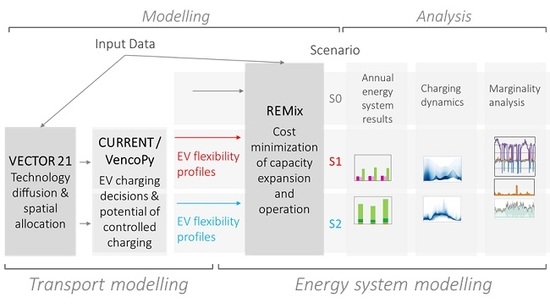
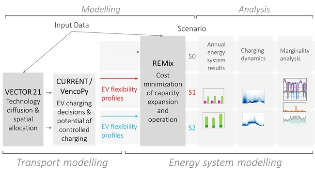
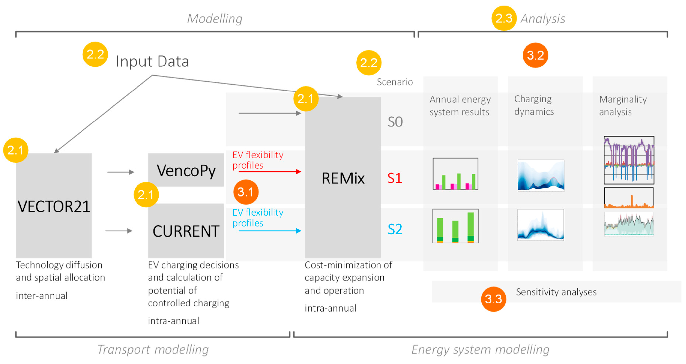
For our study, the penetration of battery EVs calculated for the year 2030 by VECTOR21 is aggregated to the two model regions considered in REMix (i.e., Northern Germany and Southern Germany).

2.1.2. Electric Vehicle Charging Models (VencoPy, CURRENT)

User-optimal BEV charging strategies are not necessarily system-optimal strategies [7]. Therefore, the consequence and differences of both approaches have to be considered in order to assess challenges and opportunities of high BEV-penetration scenarios and to draw conclusions on the detail of representing BEV charging for energy system optimization models.

In our paper, we compare two methods to simulate charging behavior of an electric fleet and then evaluate the influence of these different approaches on the energy system. First, we apply VencoPy (Vehicle Energy Consumption in Python), which is the original data preparation tool in the energy model REMix to simulate EVs and its load shifting potential in high temporal detail. VencoPy accounts for the electric demand of an electric fleet, but the charging decision and the average battery level of the fleet is determined by the power system. Second, we implement an existing transport model, CURRENT, which simulates charging behavior from a utility based approach, within the framework of REMix. This replaces the existing approach with VencoPy and accounts for detailed user behavior. We next present both models in detail. VencoPy does not directly calculate BEV charging but rather a best-case yielding high flexibility and a worst case yielding low flexibility for the energy system. Thus, when we talk about BEV charging in VencoPy’s results, we mean charging in its two respective cases.

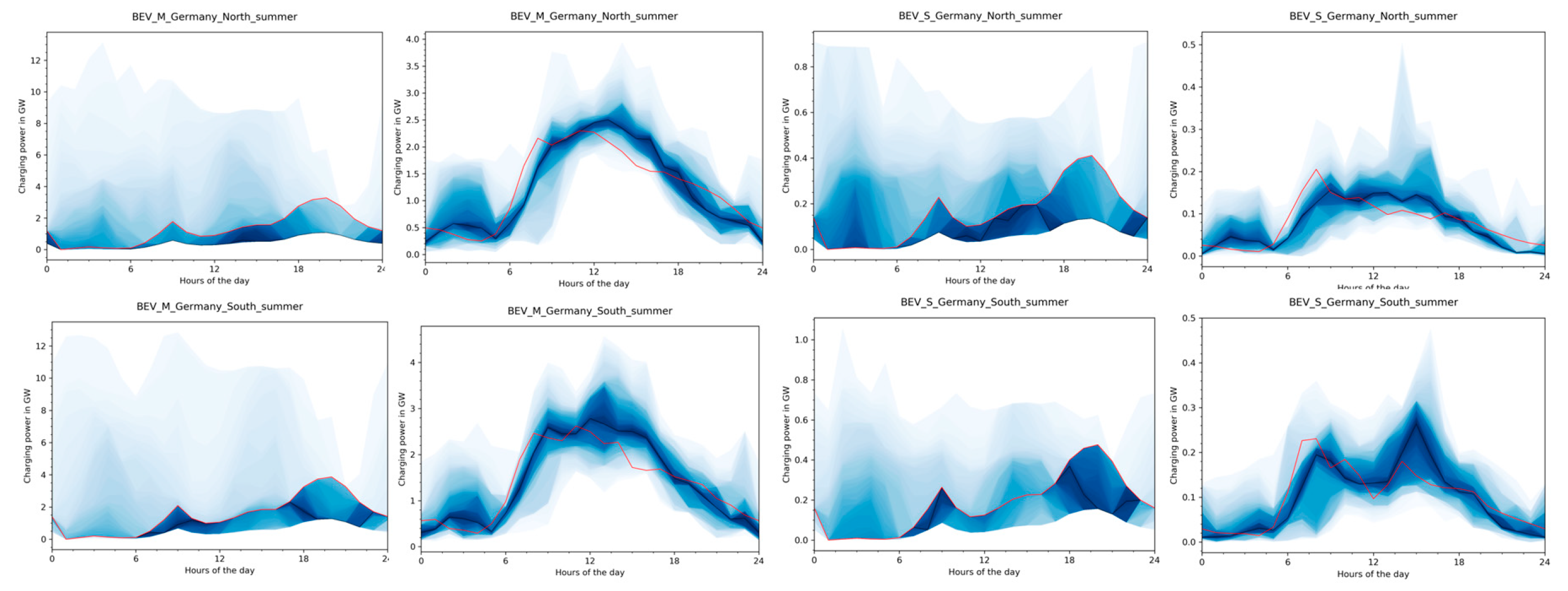
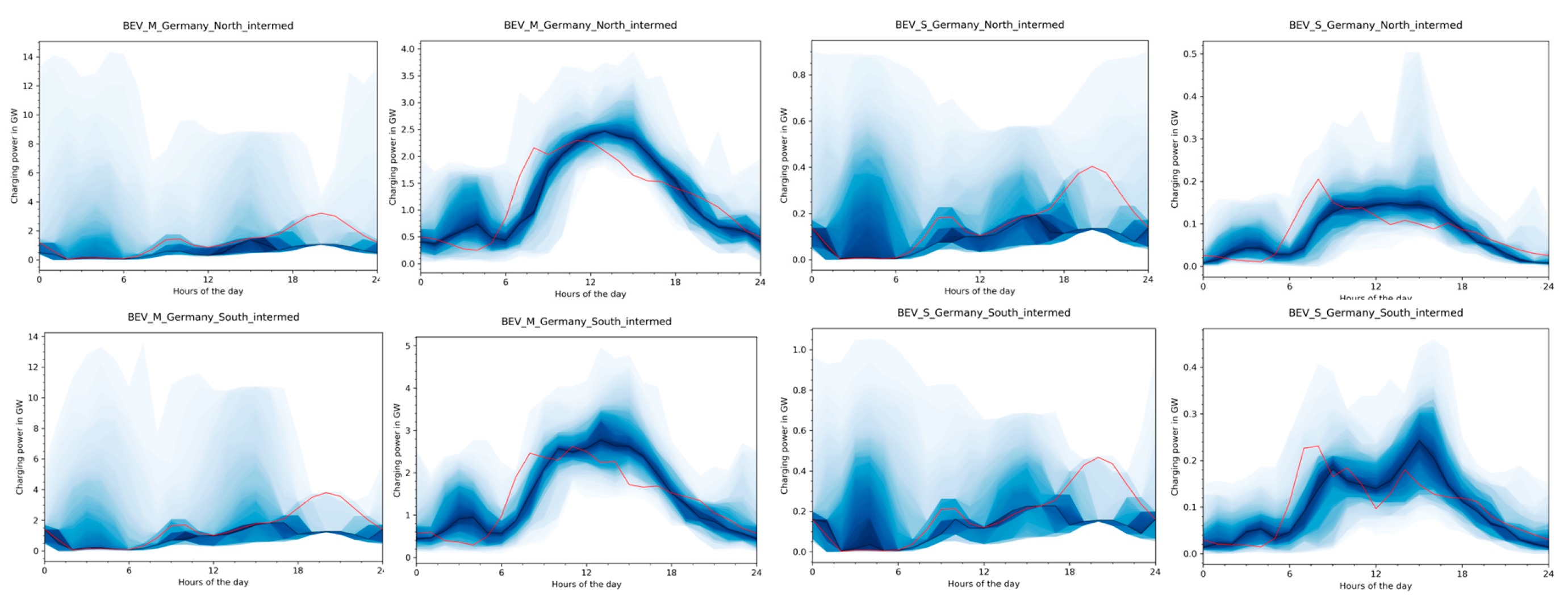
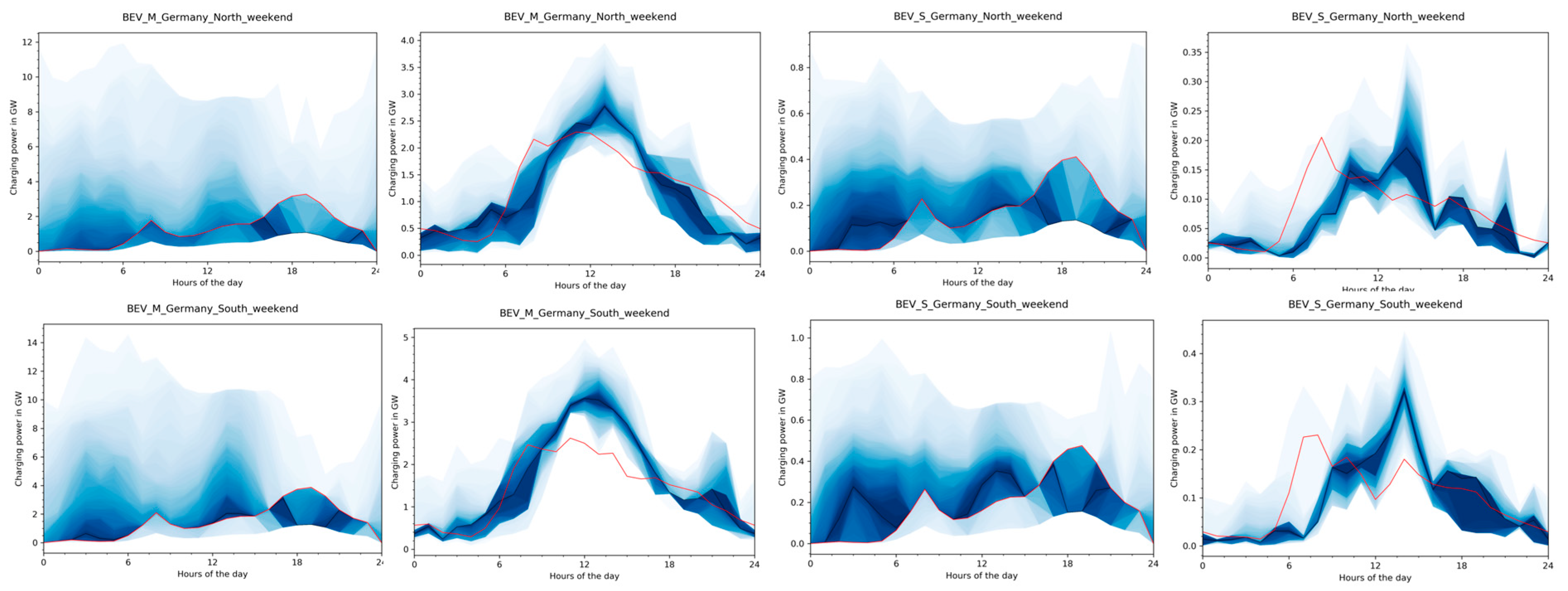
VencoPy calculates BEV flexibility profiles constraining fleet battery charging and discharging for controlled charging in hourly temporal resolution. Only home charging is assumed with vehicle segment-dependent power (small, medium, large, see Table 4). This approach is backed by empirical findings, showing a 72% of charging energy is from home charging [27]. Long-distance trips requiring fast charging events are excluded from the analysis. VencoPy calculates the hourly information of electric mileage, if a BEV is connected to the grid, and the maximum and minimum battery SOC possible to realize all travel demand. Demand data is taken from the trip dataset of the German travel survey for German household transportation demand (MiD) [23]. The maximum SOC level profile represents a case where BEVs always charge when possible with maximum SOC at beginning of the day, while the minimum battery level describes the opposite case of minimum SOC and only needed electricity for the next trips is charged before departure. A similar approach is described in e.g., [19]. Each vehicle profile is summed unweighted and normalized to a fleet profile for one day. The share of the BEV fleet that can shift its charging demand to conduct controlled charging is exogenously defined in REMix and used as a scaling factor for the normalized profiles (see next section).

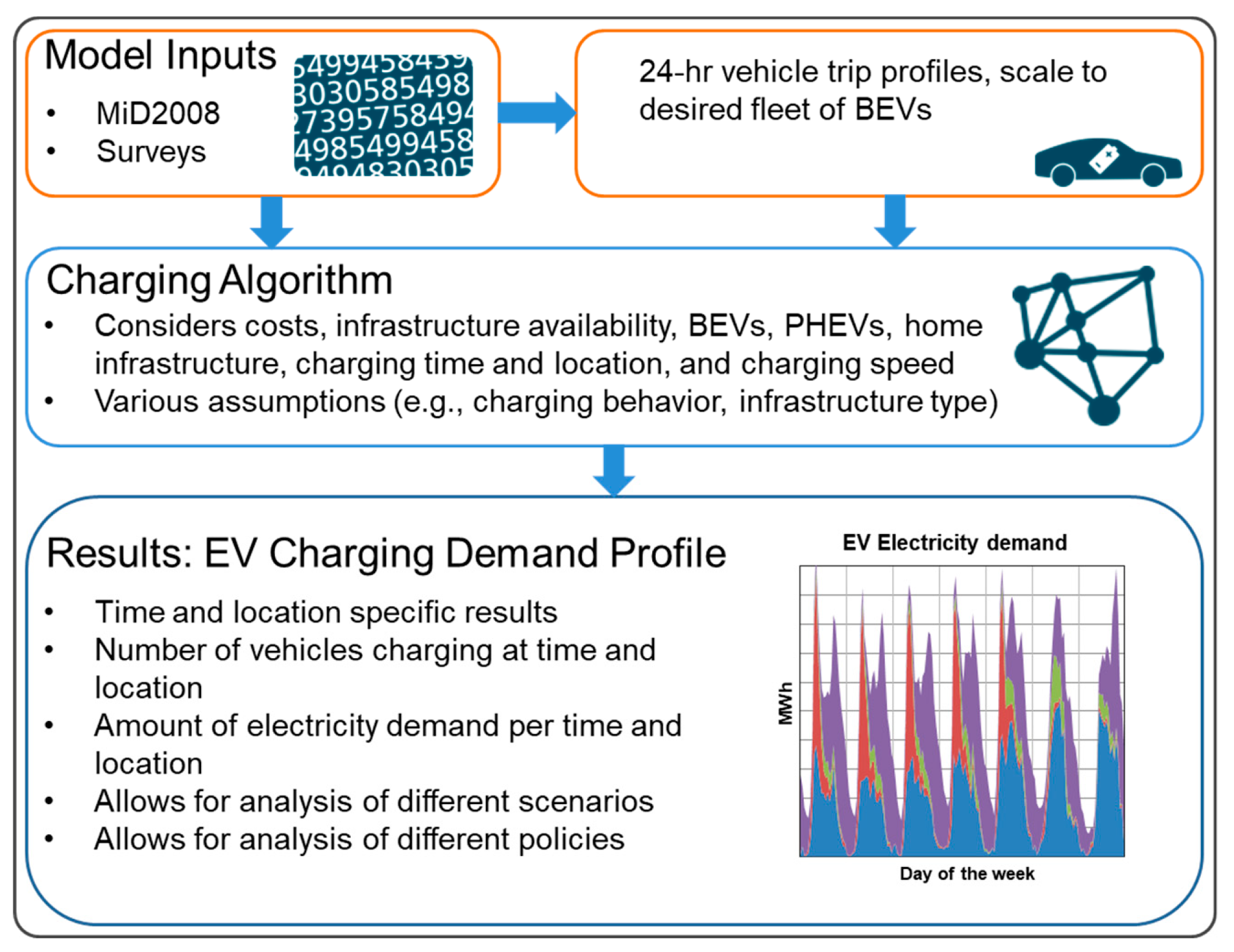
CURRENT stands for “charging infrastructure for electric vehicles analysis tool” [28]. It is a microscopic charging demand tool for BEVs providing time and location-specific information about charging [15]. CURRENT gives information on the hourly electricity demand of an electric fleet over the course of a week and shows flexibility potential for controlled charging. The overview of the model is presented in Figure 2.

Two assumptions form the basis for CURRENT’s calculations. First, BEV users do not significantly change their travel pattern. Second, users predominantly charge where they already park. These assumptions are consistent with other research [29,30] and the anticipated user behavior for a mass-market of EVs. For our case study, we use the 2008 German household travel survey (MiD) [23]. Next, we outline the workings of the model.

First, CURRENT takes the household travel dataset and creates 24-hour vehicle diaries with information for all trips and parking events for one day. Specific information for each vehicle is added to model it as an electric vehicle (e.g., electric range, charging power capacity). We then define the availability of charging infrastructure at different locations (e.g., home, work, shopping), available charging power, and a minimum parking time for a charging event. Using these assumptions and the vehicle diaries, every vehicle must run through the charging algorithm as a BEV. In the charging algorithm, every vehicle must complete every activity of the day (i.e., trip and parking event). Based on charging preferences and depending on charging opportunities during a day, a BEV is charged while parking or during a trip interruption at a fast charging station. At a fast charging event, a vehicle is charged up to 80% of its battery capacity with an average charging power of 37.5 kW. This results in an aggregated charging demand per hour of the week and per location for an entire fleet of EVs.

A charging event occurs stochastically based on a multinomial logit approach. The model enables users to account for charging preferences in their decision algorithm. A utility-based approach gives the probability of charging at each activity of the day and also for interrupting the trip for a fast charging event. The utility function of each activity considers the preference of charging per location and price per kWh. The charging decision is made by a Monte Carlo simulation according to the charging probability at the charging point. In addition, the probability of finding available charging infrastructure differs for each location (i.e., home, work, shopping, leisure, other). For each household with a vehicle and a private parking spot at home, we assign a private charging infrastructure with a maximum charging power of 7.4 kW. When interrupting a trip for a fast charging event, the probability to find a fast charging station is 100 percent. Fast chargers have a maximum charging power of 50 kW. At all other locations normal charging infrastructure with a maximum charging power of 11.1 kW is assumed. Due to a lack of empirical information, we make assumptions on the probability of finding available charging infrastructure based on [28] and assigned the information for each parking event by a Monte-Carlo simulation.

As a vehicle user does not have to charge every day—the average German daily mileage of 40 kilometers is far below an electric range of a BEV—a non-choice opportunity of not charging the vehicle on the same day is included in the choice set of the charging decision in CURRENT. The non-choice opportunity gives a probability that a vehicle is not charged every day. By simulating every vehicle diary by several sequential runs, CURRENT can simulate charging events which do not occur daily. In the end, the utility based approach leads to charging events enabled by preferences for location, price, alternatives, and current SOC. These charging events do not occur every day and at every opportunity. The calibration of CURRENT aims to get the same average SOC for the fleet at the beginning and end of the week. Further detailed information on CURRENT, all assumptions, and the detailed algorithm are summarized in [15,28].

By using the 2008 German household travel survey (MiD) VencoPy and CURRENT use the same input data. The number of BEVs by segment and region differentiated for Northern Germany and Southern Germany are harmonized for both methods and based on the results of the aforementioned stock-and-flow model VECTOR21. Also, technological assumptions of BEVs such as battery capacity, consumption, and electric range are harmonized (see Section 2.2.1).

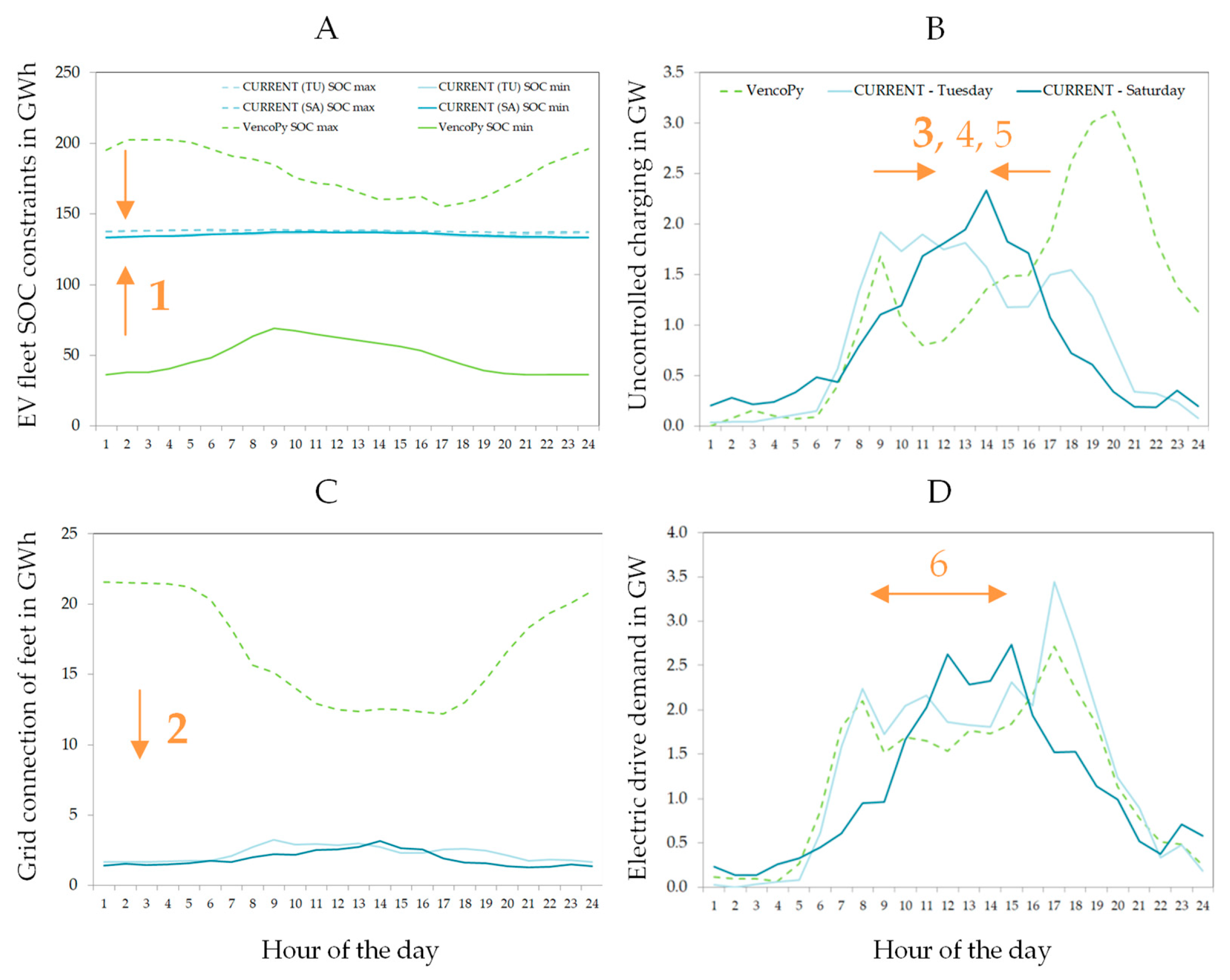
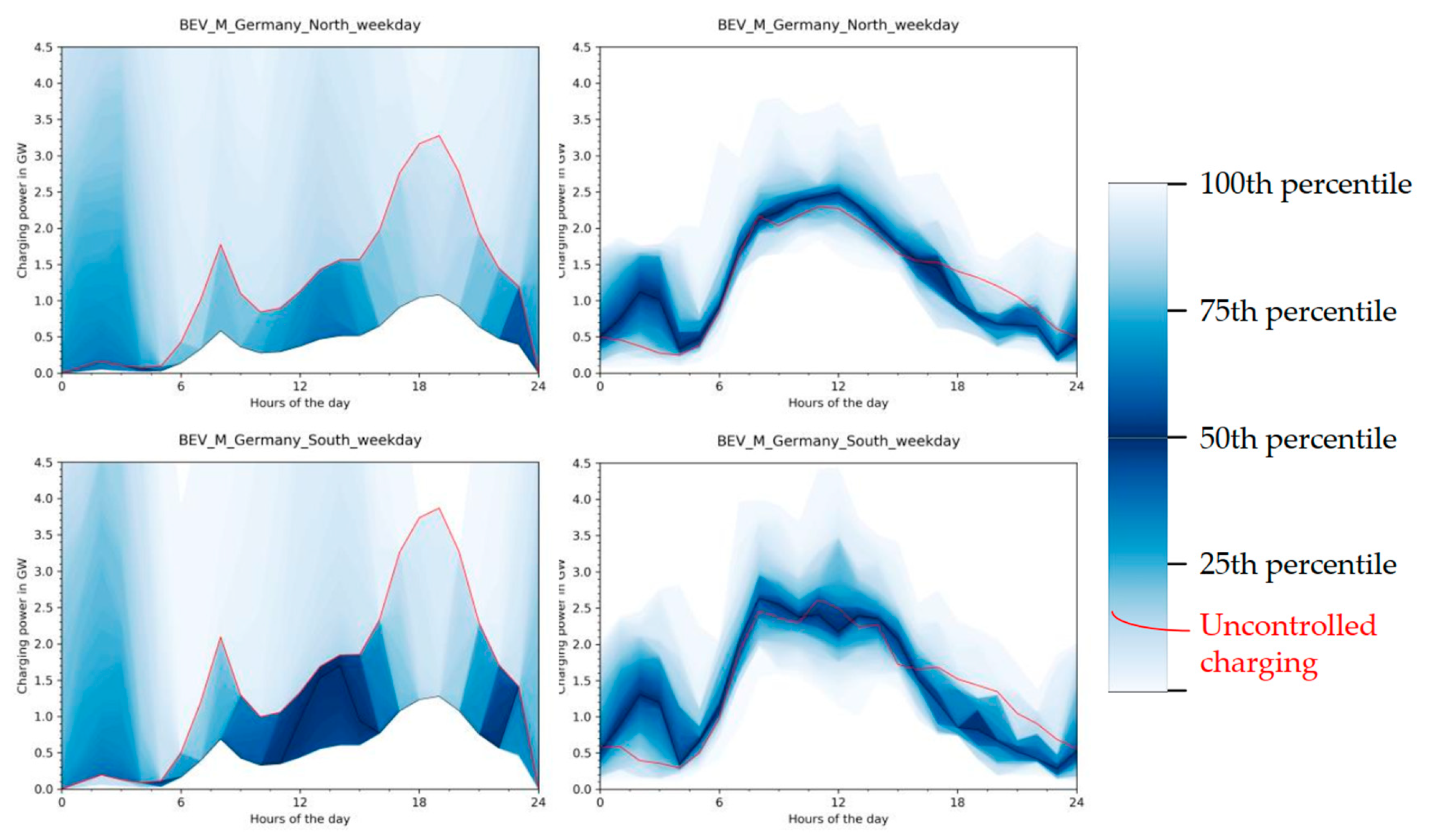
Both models differ in their degree of complexity regarding infrastructure, weekday differentiation, and users’ preferences. In comparison to VencoPy, CURRENT calculations lead to fewer charging events per day, but with the same amount of electric demand in total, and a lower number of vehicles connected to the grid because of BEV users charging and thus connecting their BEVs sufficiency-oriented in CURRENT. Also, fast charging during the trip generates a significant load due to the high charging power of each charging event and leads to high charging power during the day than in VencoPy yielding charging peaks during night hours. Fast charging events in CURRENT also give the energy system no potential to shift electricity demand, as charging time equals parking time. Since VencoPy only allows for charging at home nighttime charging is higher than during the day at other activities (i.e., work, during shopping). Allowing fast charging and charging apart from home in CURRENT, leads to more charging events during the day.

Deviating from VencoPy’s interpretation of uncontrolled charging as connecting their EV after returning home, CURRENT’s uncontrolled charging is a specific sub-part of the travel activities that require the BEV owner to recharge in order to reach sufficient SOC including fast-charging as an option of last resort. In CURRENT, minimum and maximum SOC levels of single profiles are determined via evaluating the charging time of an activity in comparison to the respective parking and thus connection time. Only if the latter is higher than necessary charging, minimum and maximum SOC profiles differ where maximum SOC represents direct charging after connection and minimum SOC the latest possible charging beginning. Thus, the power system has only little control over charging procedures under the condition of a user-oriented connection decision. This reduces the potential to shift charging demand as charging time is equal or almost equal to parking time during daytime and fast charging.

On a modeling level, a very relevant difference of the two models is their means of enforcing boundary conditions at the beginning and end of a day (VencoPy) and week (CURRENT). VencoPy assumes maximum and minimum SOC at beginning and end of a modelled day for SOC max and min respectively with a SOC security margin of 3% and secures meeting boundary conditions on each single profile basis, thus each profile and thus fleet has the same beginning and end SOC min and max. CURRENT on the other side calculates user specific SOCs for each profile under the assumption that the average BEV fleet SOC at beginning and end of the week is equal.

Table 1. Main differences between the BEV charging representation in VencoPy and CURRENT.

	VencoPy	CURRENT
Time horizon and weekday representation	1 day	7 days
BEV user representation	Demand has to be fulfilled	As in VencoPy plus temporal and activity based connection choice including non-choice option
Data and input assumptions	MiD 2008	MiD 2008
Infrastructure representation	Segment-specific rated power for home charging	Activity-specific rated power including fast-charging and availability probabilities
Boundary condition enforcement level	Single profile level	BEV fleet level

summarizes the main structural differences between BEV charging representation using VencoPy or CURRENT.

2.1.3. Energy System Optimization Model (REMix)

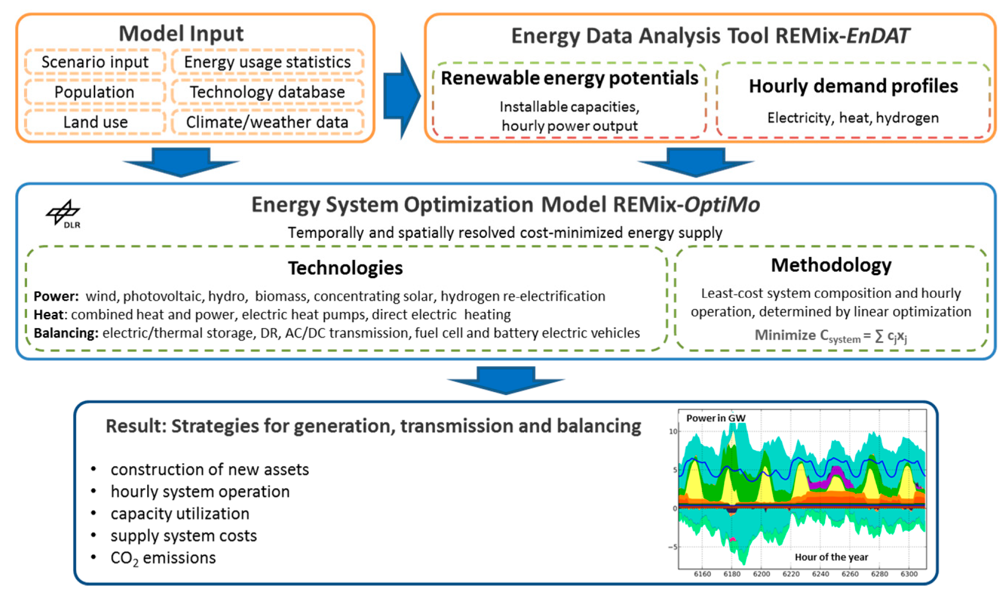
The main aim of REMix (renewable electricity mix) is to model future energy systems in high temporal and spatial resolution to adequately represent the influence of high shares of variable renewable energy sources. The model is composed of two sub models: the EnDat model for processing of input data and OptiMo to optimize the system design and operation. Figure 3 shows the main elements of the REMix model. One of the main pillars of REMix-EnDat is an inventory of renewable energy source data. It contains potentials of hourly renewable energy generation and maximum installable capacities. The model and its database are described in detail in [31]. The optimization model REMix-OptiMo relies on a linear optimization approach, which is formulated in the General Algebraic Modeling System (GAMS). The energy system is described in a system of linear equations and inequalities. The model optimizes both the hourly operation of the system during one year and the investment in additional capacities if needed to balance the energy demand. The objective function to be minimized contains the variable operational costs of all considered assets, including fuel as well as optional CO₂ emission costs, and the annuities and fixed operational costs of all endogenously added capacities.

REMix-OptiMo is a multi-node model, which implies that power generation, demand, and transmission are aggregated to predefined regional model nodes. The most important boundary condition is the power balance, which assures that power demand and supply are equal in each time step and model region. Power generation, storage, and grid technologies are represented by their cost, efficiency, availability, and maximum installable capacity. A detailed description of the general modeling approach and fundamental equations can be found in [33]. Building upon the basic model setup introduced there, REMix-OptiMo has been continuously enhanced in its scope to not only include the power sector, but also the most relevant links to the heating and transport sectors as described in [34].

The representation of EVs was originally developed within [22] and has been developed further for this work. Due to REMix’ modular structure, the sets, variables, parameters, and equations of the module representing BEVs can easily be activated or deactivated for the optimization model of minimizing the overall system cost.

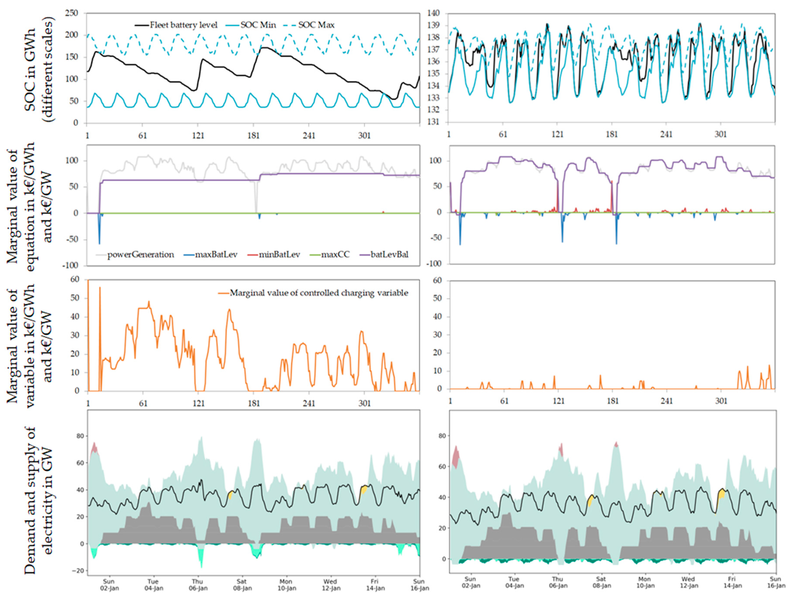
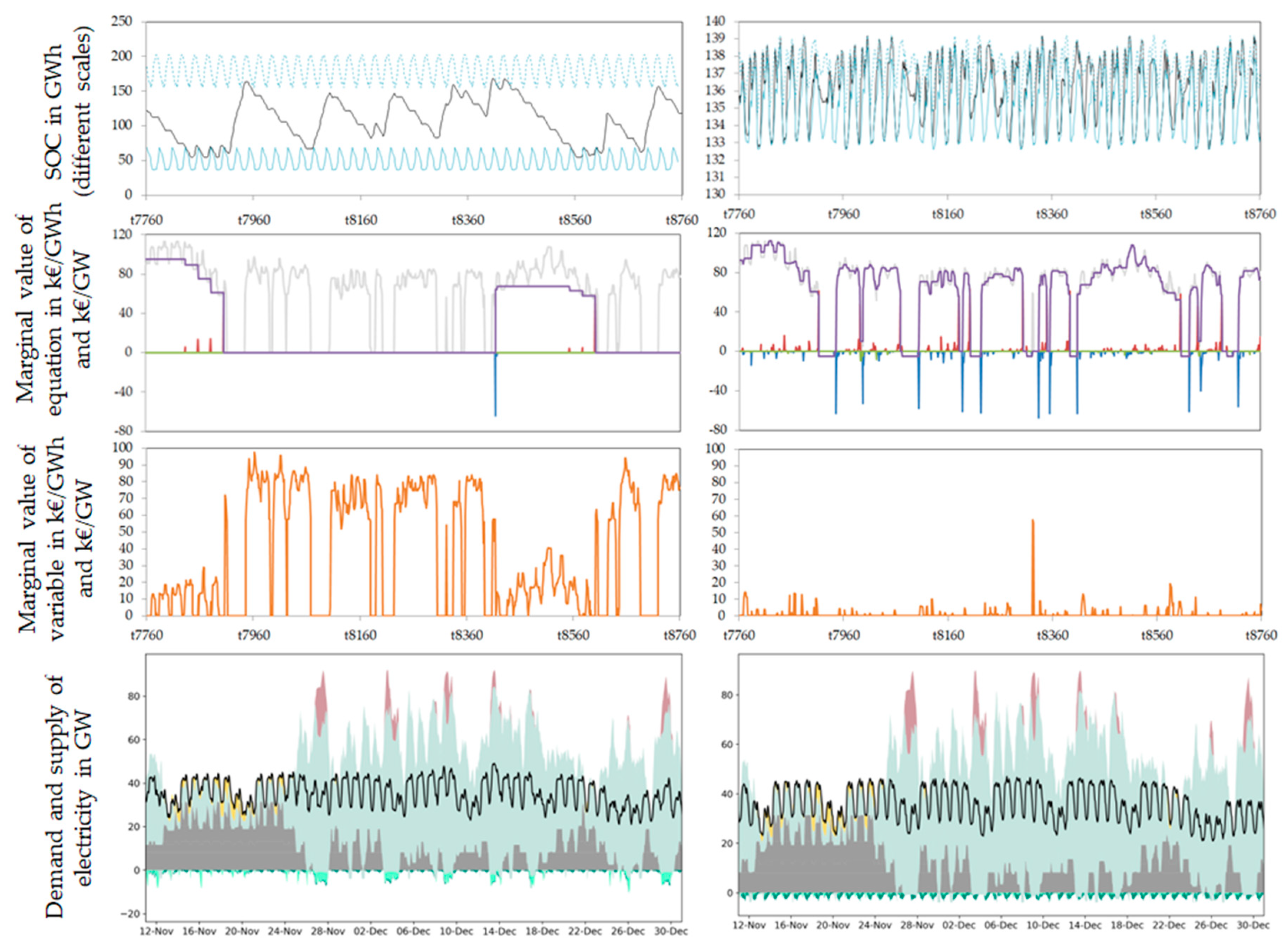
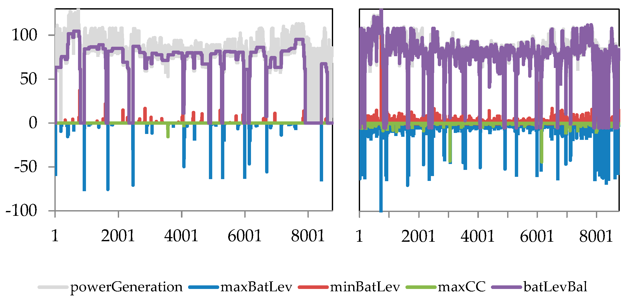
In order to represent load shifting, REMix-OptiMo requires five hourly input profiles, defining optimization constraints for charging of BEV fleet batteries. These time series input profiles contain information as follows:

• The power demand in the case of uncontrolled charging;
• The electric power demand required to fulfill mobility demand;
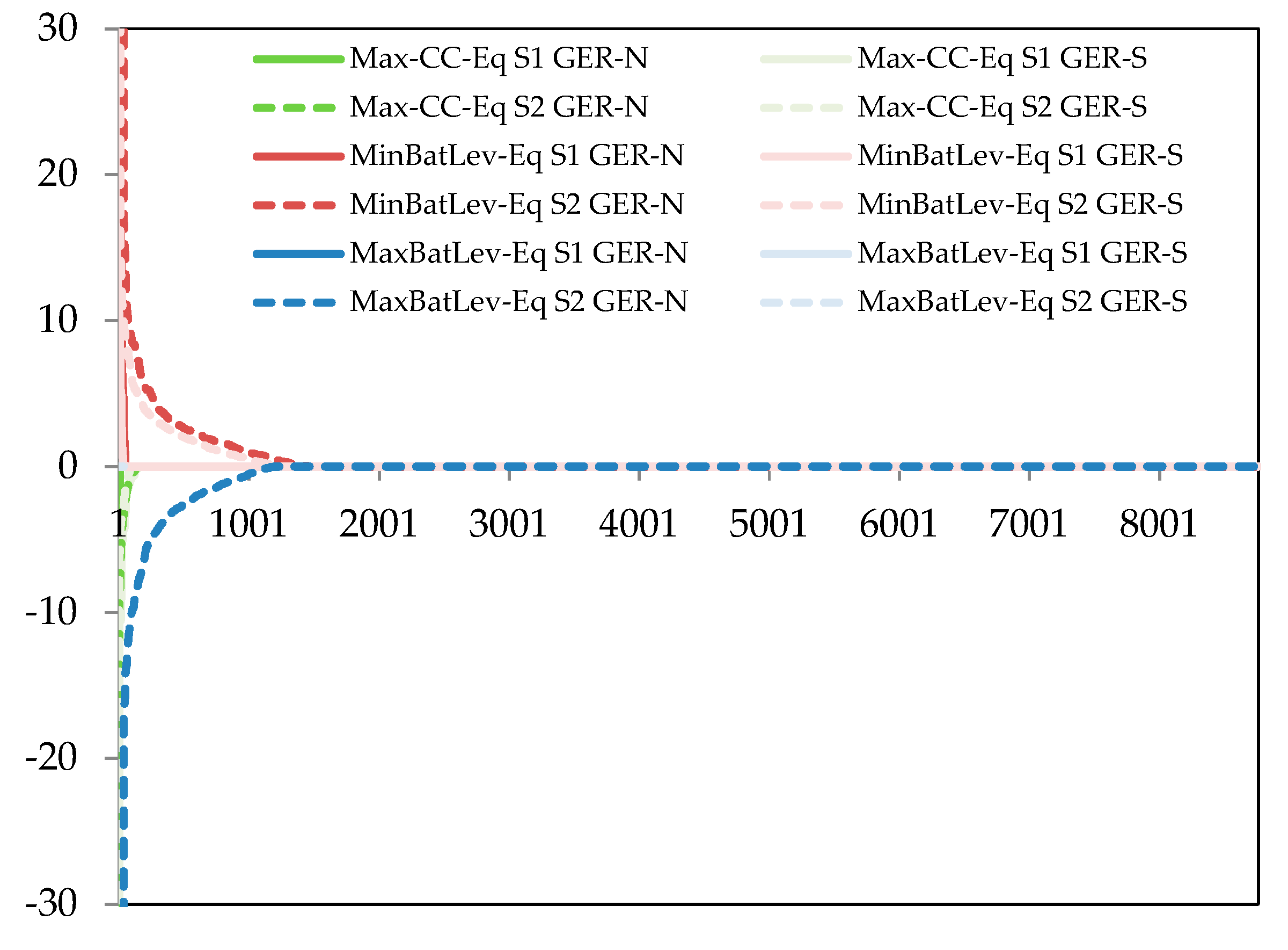
• A maximum fleet battery state-of-charge level (SOC Max);
• A minimum fleet battery state-of-charge level (SOC Min);
• The maximum rated power of the vehicle fleet connected to the grid;

More details are given in [22]. Profiles can either be given in normalized or absolute figures in units of GW and GWh. Scaling of normalized profiles to optimization input constraints is carried out in REMix’s pre-calculation phase with additional assumptions on battery capacity, vehicle numbers, charging efficiencies, and BEV segment-specific rated connection power. Non-linear effects such as the degradation of batteries depending on cycling frequency cannot be accounted for within REMix.

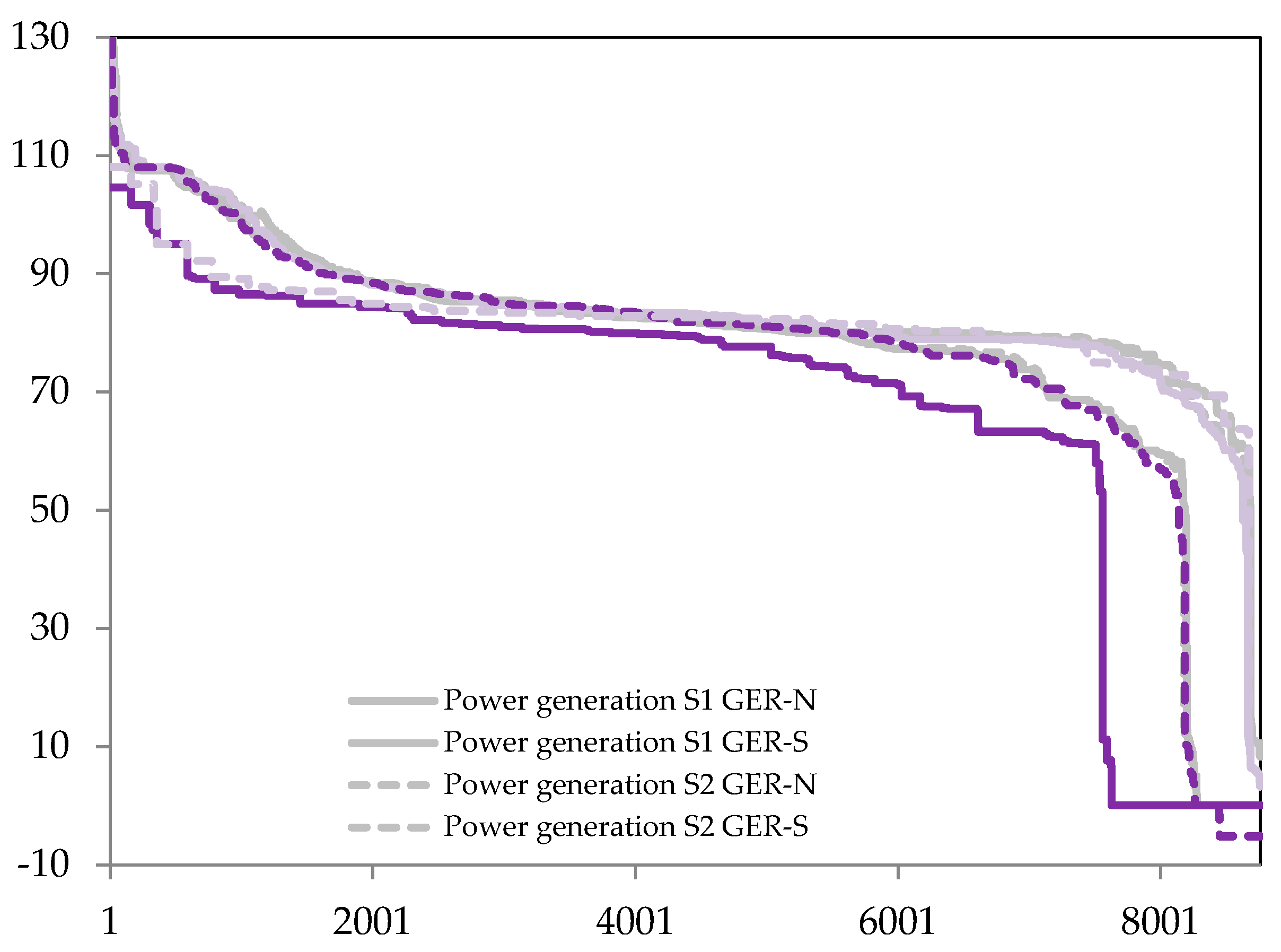
In [22], Venco provided normalized profiles with battery capacity and vehicle consumption given as input parameters. These profiles were then scaled by regional technology specific vehicle numbers, battery sizes, and consumption rates in the data preparation stage of REMix. For S1, this approach is adopted with harmonized technical and fleet-size assumptions. For S2 on the other hand, scaling from single-profile level to fleet level as well as infrastructure assumptions are endogenous parts of CURRENT calculations, thus the scaling step is skipped.

2.2. Linking the Models and Description of the Scenario Study

2.2.1. Linking the Models

Coupling the above described models requires a harmonization of dimensionality of the models, input assumptions, and at least a partial harmonization of the models’ scopes. This requires parallel runs of the lower resolution model across the higher resolution model dimension, aggregating results of the higher resolution model or selecting a relevant subset of the high-resolution dimension. Additionally, data processing steps—such as normalization, scaling, and reformatting—are needed. Harmonizing the model scope is the most challenging harmonization technique since often model endogenous specifics have to be adjusted.

Table 2. Model dimensionality and respective harmonization approaches.

Dimension	VECTOR21	REMix	CURRENT	Harmonization Approach
Spatial horizon	Germany	Germany plus neighboring countries	Germany	-
Spatial resolution	ZIP code areas	Germany in 2 nodes, others in 1 each	1 node	Aggregation of ZIP code areas to 2 nodes in Germany
Temporal horizon	2010–2050	1 year in 2030	7 days in 2030	Filtering for 2030, cloning CURRENT output for REMix
Temporal resolution	Annual	Hourly	Activity/hourly	No model harmonization between VECTOR21 and the other models, CURRENT-adaption to hourly output
Technological resolution	3 drivetrain technologies, 3 vehicle sizes	Transport: 6 technologies, Power: X technologies	1 technology	Filtering BEV, parallel CURRENT runs for each REMix-technology
Infrastructure resolution	Input to agent’s preference	1 plug power value per transport technology	Probability distributions of plug power availability depending on places	No harmonization with VECTOR21, REMix-adaptation to be able to model CURRENT output

shows the model dimensionality and harmonization approaches for respective model dimensions.

VECTOR21 model output is relevant for both REMix and CURRENT calculations, as it is taken as a quantitative input for estimating vehicle fleets of BEVs in Germany in 2030. Dimensionality mismatches are treated by either filtering or aggregation.

Cloning of CURRENT output is conducted to transfer the time horizon of a week to a full year for REMix, thereby neglecting effects of seasonal mobility behavior changes and holidays [35]. Filtering and separate runs are carried out for model regions. REMix models Germany and its neighboring countries, while surrounding countries are not relevant for modeling BEV charging decisions within Germany.

In the first scenario, S1, the BEV flexibility profiles are calculated based on the method described in [22] assuming that 94% of battery capacities of the BEV fleet are available to the power system as a battery storage. Thus, in extreme cases, each vehicle’s battery is available as battery storage with hourly varying capacity, described by profiles 3 and 4 and charge power described by profile 5 (see Section 2.1.3). In scenario S2, BEV flexibility profiles are calculated based on a harmonized CURRENT run, taking into account agent’s preferences with regard to charging location and the SOC.

2.2.2. Description of the Scenario Study

This section summarizes the main structural and quantitative model assumptions for our case study of a hypothetical German power system in 2030 including its neighboring countries. We start by describing the model scope and continue to present the main assumptions on the EV fleet and its power demand as well as techno-economic assumptions. The REMix parametrization builds upon assumptions and data given in [36].

We apply a model setup with two model regions for Germany (North and South) and its neighboring countries (i.e., Austria, Belgium, the Czech Republic, Denmark, France, Luxembourg, the Netherlands, Norway, Poland, Sweden, and Switzerland). The division into Northern Germany and Southern Germany is done to analyze the impact of the different renewable power plant portfolios. Southern Germany is dominated by wind power with approximately twice as high wind than PV installations while this relationship is inversed in Southern Germany with PV fluctuating in diurnal day and night patterns. Total fluctuating RES capacities before optimization are more than three times higher in Northern Germany compared to Southern Germany. The division of Germany is based on 21 sub-control zones of the four German transmission system operators (TSOs) [37]. Since our focus lies on differences in representation of a hypothetical EV fleet and their respective impacts on power system modeling, the German neighboring countries are taken as constant boundary conditions, even though investments in power plants and storage are allowed. Grid transmission capacities are based on [38,39]. Power system dispatch is cost-optimized for the scenario year 2030 in hourly resolution and with perfect foresight over the overall time horizon. Fluctuating RES time series are taken on the basis of calculations in [24,31,40].

We implement five conventional power plant technologies, six renewable energy technologies, as well as three storage and one transmission grid technologies as shown in

Table 3. Technology resolution of power plant, grid, storage, and EV technologies in REMix. Rows are not related to each other.

Power Plant Technologies		Grid Technologies	Storage Technologies	Electric Vehicle Technologies
Fluctuating renewable energies	Photovoltaic, wind onshore, wind offshore, run-of-the-river hydro	HVDC	Stationary lithium-ion batteries	Small BEVs
Controllable renewable energies	Reservoir hydro dam power		Pumped hydro storage	Medium BEVs
Thermal power plants	Hard coal steam turbine, lignite steam turbine, natural gas combined cycle gas turbine, natural gas gas turbine		Hydrogen underground caverns	Large BEVs

. Technology expansion is optimized in a brownfield approach based on existing capacities with the option to invest in a technology expansion to meet the power demand. Power demand from other sectors is considered only with regard to passenger BEVs.

The annual electricity demand data are taken from the European Network of Transmission System Operators (ENTSO-E). Values are disaggregated by German ENTSO-E profiles to yield hourly time series of electricity demand in order to account for the difference between weekend and weekday electric demand which is taken into account for BEV flexibility profiles in S2 as well.

In the following, we describe the quantitative basis for modeling the power system flexibility of a future EV fleet. For scenarios S0 and S1, the annual power demand from the BEV fleet has to be explicitly given and scaled in the pre-processing phases of REMix, while for scenario S2 the total EV fleet power demand is an implicit result of CURRENT. Thus, S0 and S1 input assumptions have to be harmonized in order to assure comparability across all scenario calculations. Results of the harmonization are shown in the fourth column in Table 5.

Technical assumptions that are constant for all model regions for scenario S1 are shown in

Table 4. Technology assumptions for EVs for scenario S1 and respective degree of harmonization with scenario S2 input assumptions. Battery capacity values are assumed based on a comparison of historic battery sizes and literature projections from [18,20,28,41,42].

Name		Unit	Value	Degree of Harmonization
Battery capacity (gross)	BEV-S	kWh	40	harmonized
	BEV-M	kWh	70
	BEV-L	kWh	100
Charging capacity	BEV-S	kW	3.7	Not harmonized
	BEV-M	kW	7.4
	BEV-L	kW	22
Electric demand	BEV-S	kWh/km	0.15	harmonized
	BEV-M	kWh/km	0.20
	BEV-L	kWh/km	0.25
Share of controlled charging		%	67	Not harmonized
Efficiency of vehicle charging (plug to battery)		%	95	harmonized
Variable operation and maintenance costs of controlled charging		€/MWh	5	harmonized

. Battery capacity assumptions are compared to historic values, ranges given in the IEA EV Outlook 2018, and to literature assumptions on prospective values in Figure A2.

We assume that two-thirds of the vehicles can be charged by controlled charging following an upper-bound assumption from [9], limiting the flexible charging demand to approximately 18 TWh/a. A REMix-endogenous model decision regarding the investment enabling controlled BEV charging is not considered as we are foremost interested in intra-annual implications of user behavior and increased detail of representing infrastructure. A harmonization of BEV fleet shifting capabilities will be presented in a sensitivity analysis.

Table 5. EV fleet spatially dependent parameters as aggregated results from VECTOR21 scenario.

Model Node	Vehicle Size	Number of Vehicles in Units of 1000 Vehicles	Annual Electric Demand in TWh/a
Northern Germany	BEV-S	414	1.31
	BEV-M	3365	10.68
	BEV-L	215	0.68
Southern Germany	BEV-S	492	1.52
	BEV-M	4078	12.61
	BEV-L	213	0.66
Sum	-	8777	27.47

presents VECTOR21 results for the BEV vehicle fleet aggregated to REMix model nodes for 2030. For matching geographical boundaries data from [43] was used. With a cumulated BEV fleet of 8.8 million vehicles in 2030, we assume a stronger BEV adoption than the one given in the scenarios for the European 10-year network development plan of 2.6–5.4 million EVs for Germany [44].

In scenario S1, we assume two-thirds of the BEV fleet as flexible fleet battery that can be mostly charged controlled top-down by the power system needs within the given SOC min and SOC max profiles as described in Section 2.3. In S2, we describe the charging patterns and behavior-related decisions of representative agents and thus the BEV fleet only provides a load shifting potential at times where the parking duration exceeds the charging duration.

Charging connection power of size specific BEV fleets and the share of controllable charging procedures of the fleets are not harmonized between scenarios S1 and S2. Since CURRENT simulates both infrastructure availability and user preference to connect a respective vehicle to the grid at a given location, plug power, and the controlled charging share are both determined endogenously and resulting hourly week-profiles are cloned to the annual timescale and formatted taking into account weekday specificities for adjustment of BEV profiles to other sectors’ electricity demand profiles.

2.3. Analytical Methods

We analyze the effects of differing BEV charging representation on annual energy system modeling results, on detailed sub-annual BEV charging characteristics and shed light on the changing role of the BEV fleet throughout the year by analyzing the marginal values of model equations and variables. Since energy system optimization modeling results are sensitive to GHG ambitions, the underlying weather and demand data and techno-economic assumptions, we then calculate the same model setup with three additional degrees of GHG ambitions, six additional weather and electric demand years between 2006 and 2012, and two other sets of capital expenditures for fluctuating RES technologies. With this, we test the robustness of shifted energy and annual energy system results. In this section, we describe our methodological approach to analyze REMix model results.

REMix model results are partly transformed in its post-calculation phase, yielding .gdx files. These are again aggregated using a Python script, writing pivot-table data to excel files. For analysis, multiple result files are then combined in an analysis file giving tabular data with filtering, aggregation and different visualization methods. These files are used for the analysis of REMix results on an annual basis. Peak load and information about imports and exports are extracted individually from the .gdx files.

A separate evaluation framework is set up for the analysis of sub-annual BEV fleet charging characteristics. The calculation of shifted load is carried out in this framework since the shifted load is calculated slightly different in S1 and S2. In S1, the shifted power is calculated as shown in powerShiftVP

$$\mathrm{shifted}\mathrm{power}\left(\mathrm{S}1\right)={\displaystyle \sum }_{t=1}^{8760}R\left(t\right)-{\Psi }_{CC}\left(t\right)$$

powerShiftVP

with R(t) being the cumulative charged energy of the vehicle fleet in each hour in the case of uncontrolled charging and Ψ_CC(t) being the real electric vehicle fleet charging energy. In S2, shifted power is calculated taking into account two of the BEV flexibility profiles, uncontrolled charging, and the maximum battery SOC

$$\mathrm{shifted}\mathrm{power}\left(\mathrm{S}2\right)={\displaystyle \sum }_{t=1}^{8760}\left[\left(C_{unc}\left(t\right)+{\mathrm{L}}_{max}\left(t\right)-{\mathrm{L}}_{max}\left(t-1\right)\right)-{\Psi }_{CC}\left(t\right)\right]$$

powerShiftCU

with:

• C_unc: Uncontrolled charging (battery inflow) of BEV fleet;
• Ψ_CC/Ψ_V2G: Controlled charging of BEV fleet battery in the case of only controlled charging (CC) or with the option to feed electricity back to the grid (V2G);
• Φ_V2G: Electricity fed-back to the grid from the fleet battery;
• P_drive: Exogenously given electricity demand for driving in each hour;
• Λ(t): Battery level in hour t.

In linear optimization, results comprise not only the value of variables at the optimal solution, but also the value of marginal changes of variables and constraints. These values are referred to as marginal values of variables and marginal values of equations (equalities and inequalities). Generally, the marginal value of an inequality is only unequal 0 if the formulated constraint is bounded, for example if the SOC is at its maximum level. Equalities are transformed to two inequalities, thus equalities are always bounded.

Marginal values of variables and equations are shortly described using the battery level balance equation in REMix where Latin letters describe exogenous parameters and Greek letters optimization variables. For clarity, the parameters’ and variables’ dependency on the model region and the vehicle segment are ignored. The equation batLevBal is

$$C_{unc}\left(t\right)+{\Psi }_{CC}\left(t\right)+{\Psi }_{V2G}\left(t\right)-{\Phi }_{V2G}\left(t\right)-P_{drive}\left(t\right)=\Lambda \left(t\right)-\Lambda \left(t-1\right)$$

batLevBal

The battery level constraints limiting the SOC of the BEV fleet are given by the equations maxBatLev and minBatLev

$$\Lambda \left(t\right)\le L_{max}\left(t\right)$$	maxBatLev
$$\Lambda \left(t\right)\ge L_{min}\left(t\right)$$	minBatLev

Finally, controlled charging must not be higher than the currently connected charging power of the EV fleet given by the equation maxCC

$$\frac{{\Psi }_{CC}\left(t\right)}{{\eta }_{GtV}}\le P_{charge, avail}\left(t\right)$$

maxCC

with

• η_GtV: Charging efficiency between the grid and the vehicle battery.

Each equation has a marginal value in the solution for each hour corresponding to the increase of total system cost if the sum of all non-variable terms is increased by 1 unit in the respective unit of the equation. For the maxBatLev equation this implies increasing $L_{max}\left(t\right)$. by 1 GWh and for batLevBal increasing $P_{drive}\left(t\right)-C_{unc}\left(t\right)$ by 1 GW, respectively.

Since there are only two variables for each hour, namely the battery level and the amount of controlled charging, the marginal values of the equations are tightly coupled to each other. When the EV fleet battery SOC is not bounded, the marginal of the battery level balance equation has the value of the last time that it was constrained minus the marginal value of either the maxBatLev or the minBatLev equation if it was at upper or lower bound respectively. Since maxBatLev marginal are always negative and minBatLev marginal always negative, the marginal value of the batLevBal equation increases by the negative value of the marginal of maxBatLev and continues on this level until the SOC reaches another constraint.

3. Results and Discussion

We now present the scenario study results as per Figure 1 and described in the previous sections. We start with an introductory quantitative and qualitative description of the differences between scenarios S1 and S2 (Section 3.1). Specifically, we examine the amplitudes and temporal distributions of the five EV flexibility profiles introduced and described in Section 2.1.2 and Section 2.1.3. We exemplify the profiles and identify three major and three minor differences in the two approaches of representing EV charging dynamics and constraints. Building on this, we describe the results of the scenario study on an annual scale compared to benchmark scenarios (Section 3.2.1) and differences in intra-annual EV charging characteristics between S1 and S2 (Section 3.2.2). We then present an analysis of the marginal values of the main equations and variables of the BEV module in REMix, providing deeper explanatory insights into the specific importance of different model details. Section 3.3 assesses the sensitivity of the insights with regard to GHG reduction ambitions, historic weather and load years, and assumed techno-economic parameters of power-plant technologies.

3.1. Comparison of BEV Flexibility Profiles (Intermediary Results)

As a basis for comparison, scenario S0 calculates benchmarking values without additional power demand and load-shifting flexibility from BEVs. The consecutive scenarios S1 and S2 assume a penetration of 8.8 million BEVs in Germany, implying an additional annual power demand of around 29 TWh including 5% electricity losses during charging procedures increasing the electricity demand given in Table 5.

Table 6. Summary of fleet power demand flexibility characteristics in the three scenarios considered (S0, S1, and S2). Cumulative power demand includes losses during charging. SOC range gives the minimum and maximum difference between SOC max and SOC min. Fleet connection share includes uncontrollably charging BEVs. For SOC and fleet connection ranges, VencoPy daily minimum and maximum hours, for CURRENT weekly minimum and maximum hours are used.

EV Charging Model (Scenario)	Cumulative Power Demand from BEV Fleet in TWh/a	SOC Range Available to Power System Load-Shifting in GWh	Fleet Connection Share Range in GW	Share of Uncontrolled Charging in %
- (S0)	0	0	0	-
VencoPy (S1)	29	272–419	33–59	33%
CURRENT (S2)	29	5–10	3–8	70%

provides an overview on quantitative implications of the two different methods of modeling BEV charging characteristics aggregated for Northern Germany and Southern Germany, as well as for all vehicle sizes. The hourly load shifting potential range describes the difference between the minimum and maximum BEV fleet SOCs in a specific hour. It is significantly reduced in S2. Explicitly modeling a non-choice and a fast-charging option leads to a reduction of the fleet connection share of the BEV fleet from a range between 33–59 GW in S1 to 3–8 GW in S2. The share of uncontrolled charging is an exogenous assumption in scenario S1, while it is a result of CURRENT’s microsimulation in scenario S2.

The following

Table 7. Structural differences in BEV charging representation between VencoPy and CURRENT. Shown are structural differences in the models VencoPy and CURRENT.

	Number	Representation Detail	Quantitative Effect on BEV Flexibility Profiles
Major structural differences	1	Weekly boundary conditions for BEV fleet SOC	Reducing available aggregated BEV fleet battery capacity for load shifting from minimum 272 GWh to maximum 10 GWh
	2	Taking into account users’ sufficiency-oriented charge connection	Reducing grid connection of BEVs from 33 GW min to 8 GW max
	3	Including fast-charging	Reduction of controllable charging by 16.2 TWh/a
Minor structural differences	4	Possibility to charge at other locations than home	Shifts charging availability from night to daytimes
	5	Accounting for non-availability of private home charging infrastructure	Reduction of total charging availability and shifting charging to daytime
	6	Accounting for weekday-specific travel patterns	Effects on all profiles (see text)

systematizes the above described structural differences in BEV charging modeling.

Including fast charging in CURRENT in comparison to VencoPy leads to an increase in uncontrolled charging since charging time is always as long as parking time for fast charging. The additional degrees of detail that were added to the simulation in CURRENT are other charging locations such as work and shopping, more realistic probabilities of availability of home charging infrastructure, as well as a differentiation between weekday-specific travel patterns. The expansion of time horizon from one model day in VencoPy to a week in CURRENT affects all profiles. Uncontrolled charging and grid connection are shifted to later times in the day during weekends. BEV owners drive more during the day and less during the morning and evening, which shifts electric demand to daytime hours. Load shifting potential increases during daytime hours on the weekend due to more BEVs being parked at home and available for load-shifting. EV flexibility profiles are depicted in Figure 4 for S1 and S2.

Constraining BEV fleet SOC profiles are shown in Figure 4A. There is a significant reduction in BEV fleet battery capacity available to the power system for load shifting from 270–420 GWh in S1 to 5–10 GWh in S2. This reduction is mainly explained by the first major effect of different boundary condition enforcement and aggregation procedures in VencoPy and CURRENT (see Section 2.1.2 and Table 7).

In Figure 4B, the influence of effects 3, 4, and 5 can be seen. Uncontrolled charging is shifted to daytime hours through fast charging and other charging locations and a probability that no charging option is available at home. Additionally, the influence of working day and weekend transportation demand is shown in the CURRENT profiles resulting in a 2:00 p.m. peak on Saturdays while uncontrolled charging reaches a slightly-decreasing plateau between 8:00 a.m. and 7:00 p.m. on working days.

The difference in charge connection profiles shown in Figure 4C originates from two causes. VencoPy assumes, that only home charging is allowed, but that BEV users connect their vehicles as soon as they arrive home with the rated connection capacities given in Table 4. This leads to a high fleet charge availability during night hours and an approximately 50% fleet charge availability from ~10:00 a.m.−6:00 p.m. when users start returning home. In CURRENT on the other hand, BEV users only connect their vehicle when it is required by their respective trip purposes, thus adjusting their grid connection to their respective mobility needs. This explains the overall lower fleet connection share. The reversed course of the graphs in Figure 4C is due to a more detailed non-vehicle-size-dependent infrastructure modeling in CURRENT. Fast charging is taken into account which amounts to 59% of the total charged electricity and thus significantly shifts vehicle connection from nighttime to daytime hours. Additionally, probability distributions are assumed for the charge connection availability at the places home, work, shopping, and other activities.

Electric driving demand profiles are found to be similar as shown in Figure 4D. Slight differences evolve from CURRENT’s differentiation in weekdays as well as the consideration of weights of representativeness that are given in the dataset both of which are neglected in VencoPy aggregation procedures from individual profiles to BEV fleet aggregates.

The analyses of the two methods (power system-oriented approach versus user-behavior-oriented approach) have some limitations. First, the results rely on conventional travel patterns. We assume that electric vehicle users do not alter their travel patterns. This assumption is supported by the literature, but we are also limited by the lack of data on detailed travel information of electric vehicle users [29,30]. Second, electricity demand from BEVs is temperature and seasonally dependent, which was not considered in this model experiments but suggested, e.g., in [4]. Third, assumptions for user-preferences are based on a specific study from Australia [45]. Fourth, capacity limits of medium and low voltage distribution grids connections are not taken into account. Fifth, CURRENT makes very conservative assumptions on grid connections, which are only taken from the driver’s perspective and when charging is needed.

Future work should focus on isolating each effect given in Table 7, thus giving the chance of decisively quantifying the implications of integrating each aspect into BEV charging modeling. Additionally, empirically measured charging behavior of BEV users could be taken into account to gain insights on real BEV users’ behavior. Additional inter-seasonal effects such as electricity demand by vehicle heating and cooling [4,7] as well as travel behavior due to holidays [35] should be evaluated on their respective importance to load shifting potential of future BEV fleets.

3.2. Implications of Structural Differences in Representing BEV Fleets

In this section, we give three key implications of the different model approaches on annual energy system model results, intra-annual BEV charging, and on intra-annual importance of the respective equations. Each main insight is given at the beginning of each section and then described and discussed in the following for easier readability. All results are available as .gdx files in the data Appendix A.

3.2.1. Energy System Implications on an Annual Basis

In the following, we describe the results of three scenarios (S0, S1, and S2) and thus the implications of the different modeling approaches on energy system modeling results. We find that fast charging and the reduced BEV fleet battery capacities have the strongest influence on energy system results, significantly reducing BEV fleet flexibility provision from 24 TWh in S1 to 8 TWh in S2 shifted load. Other flexibility options such as curtailment (+31% curtailed energy) and gas power plants (+5% in capacity additions) compensate for lower BEV fleet load shifting potential.

Table 8. Overview on scenario definitions and main annual results of the four main scenarios under analysis. Total system costs are given for the complete system boundary while all other values are given for Germany. Difference in total system costs between S2a and S2 is more than an order below numbers shown. Source: Own calculations.

	Scenario Definitions				Results
Scenario	Annual Electricity Demand from BEV Fleet in TWh	Controllable Share in %	Total System Costs in bn. €	Shifted Load by German BEV Fleets in TWh	Peak Load in GW	Installed Capacities of Power Plant Park in GW	Installed Fluctuating RES Capacities in GW	Fluctuating RES Capacity Additions in GW	Gas Power Plant Capacity Additions in GW	Annual Power Generation in TWh	Annual Fluctuating RES Power Generation in TWh	VRE Share in Total Power Generation in %	Annual VRE Curtailment in TWh	Imports to Germany in TWh	Exports from Northern G to Southern G in TWh
S0	0	-	68.4	0	83.9	214	153	46.2	31.3	501	279	55.7	2.9	45.9	64.7
S1a	27	0	71.7	0	91.1	224	156	49.0	39.0	525	284	54.1	3.6	50.3	62.9
S1	27	66	71.2	24.2	86.3	223	159	51.5	35.5	526	291	55.3	2.6	51.3	65.1
S2a	27	0	71.7	0	93.5	223	156	48.8	37.9	524	284	54.2	3.5	51.6	62.4
S2	27	30	71.7	8.4	87.6	222	156	48.8	37.2	524	284	54.2	3.4	51.6	62.2

shows the results of the scenarios S0, S1, and S2 including two intermediary benchmarking scenarios S1a and S2a, where additional BEV electricity demand occurs without any load shifting potential for the same scenario study boundary conditions and temporal VencoPy and CURRENT profiles (green lines in Figure 4) respectively.

Total system costs increase by approximately 5% induced by an additional electricity demand from German BEV fleets. This increase can be reduced to 4% by controllable BEV charging with high control through the power system. Total system cost values for uncontrolled and user-behavior constrained charging are similar. In S1, additional load is compensated by both gas turbine and onshore wind power capacity expansions that can be well balanced by the fleet shifting potential. A higher peak demand occurs when introducing additional BEV electricity demand. Complete inflexibility increases peak demand by 7.2 GW or 9.6 GW in S1a and S2a respectively. Assuming BEV fleets’ controlled charging decreases the peak load by 4.8 GW (S1) and 5.9 GW (S2).

Due to lower flexibility especially on an 3–4-day timescale, in S2 5% lower onshore wind capacity expansions (−2.7 GW) have to be compensated by increased gas turbine expansions of 5% (+1.7 GW) reducing the RES share in power generation slightly from 55% to 54%. Gas turbine additions are around twice as high in northern Germany. Reducing the BEV fleets’ flexibility further increases gas power plant needs by 0.7 GW in Southern Germany and around 1 GW in Northern Germany. At the same time, curtailment is increased from 2.6 TWh in S1 to 3.4 TWh in S2 indicating that despite 2 TWh lower wind power feed-in, the decreased charging controllability leads to a significant amount of hours in the year where wind oversupply cannot be stored in the BEV fleet.

Import levels are comparable in S1 and S2 and lie around 12% above the benchmark values. Main importers of electricity to Germany are France, Sweden, Switzerland, and Norway. Germany exports electricity to Poland and the Czech Republic. Inner-German electricity transport is high at above 60 TWh from Northern Germany to Southern Germany in all scenarios. It is higher in S1 due to lower power generation from conventional power plants in the south (−4 TWh) but also in the north (−2 TWh).

Especially the decreased BEV fleet battery capacity available for load shifting leads to a significant reduction in quantity and quality of flexibility provision of BEV charging. Load in S2 can only be shifted diurnally within a day thus diminishing the BEV fleet’s potential to balance wind power feed-in. This effect of future BEV fleets as a complementary PV balancing option has already been described by [4,46]. Coal power plant generation is slightly increased in Northern Germany by 1.3% and 1% for coal and lignite plants respectively and reduced by 2% for coal power plants in Southern Germany.

Curtailment reductions found in [17] are lower even in S1 when high flexibility is assumed. Peak load reductions are higher which can be explained by the assumptions of very high BEV penetration rates, considering their 40 kWh BEV battery as the smallest size with the majority being at 70 kWh. The different assumptions in charging power of our 3.7, 7.4, and 22 and fast-charging is supposedly not very relevant because of the unimportance of the charge connection constraint (see next section).

Future work should take into account BEV fleets in neighboring countries, empirical indications of BEV users’ adoption of controlled charging and respective economic incentives as well as feedback of power generation costs to the users to assess to what degree BEV users could be incentivized to system-friendly charging by price signals.

3.2.2. Energy System Implications on Charging Dynamics

Charging dynamics vary significantly between S1 and S2 as well as Northern Germany and Southern Germany as shown in the following. Reduced BEV fleet battery capacity has the strongest influence on charging profiles resulting in a significantly reduced variability. Including fast charging, the non-choice option and other daytime charging options lead to higher daytime charging peaks. Accounting for differences in weekday travel patterns lead to increased weekend daytime hour charging in Northern Germany (+40%) and Southern Germany (+12%) and to a sharper peak at 1 p.m.

For the power system, three main implications result from BEV usage. First, the mileage of an electric fleet imposes an increased electric demand in each hour for the energy system. Secondly, BEV charging events and the respective fleet grid connection power available are subject to temporal dynamics. Thirdly, controlled charging may occur when the time that a vehicle is connected to the grid is longer than the time required for a complete charging process and thus, the beginning of a charging event can be shifted to a later point in time.

As CURRENT differentiates each day of a week, the BEV electricity demand differs in particular from working days and weekend. For example on Sunday only 54% of the vehicles are used, while during the week the share of vehicles with a minimum distance driven is 70%. Not only the number of vehicles used is different for each day of a week, also travel pattern and time of travelling, which results in different time and location a charging event occurs.

Figure 5 shows the daily charging patterns for all working days of the year differentiated in charging in Southern Germany and Northern Germany for a cost-optimal charging with high controllability by the power system (S1) on the left and lower flexibility (S2) on the right-hand side.

Even though uncontrolled charging input profiles are very different, a few similarities can be observed. Generally, electricity demand is shifted from morning and evening hours to midday and nighttime hours. In S2, the reduced BEV fleet battery capacity leads to a sharply reduced variability of controlled charging power from up to 14 GW (beyond y-axis cutout of S1) to around 4.5 GW.

Between 6:00 and 9:00 a.m. the median of controlled charging is at its minimum in both scenarios. For evening hours, this is true for the timeframe between 5:00 and 9:00 p.m. for the high fleet flexibility since the evening load peak occurs in the same time interval (compare Figure 4). For scenario S2 the median is not as sharp at the bottom, which is due to varying weekday-dependent travel patterns but generally up to 1 GW below uncontrolled charging. From midnight on, charging occurs to a higher degree than in the uncontrolled charging case although uncontrolled charging reaches its minimum around 4:00 a.m.

The controlled charging median is much higher in S2 (1.1 GW in Northern Germany and 1.4 GW in Southern Germany) compared to 0.2 GW in S1 due to many working day nights in S1 where charging is not needed at all, even though electricity load is low. A strong alignment of controlled charging to PV feed-in can be observed in Southern Germany versus Northern Germany for S1. For S2, this effect is also observable, yet not as strong and complimented by generally broader charging behavior during daytime in Southern Germany compared to Northern Germany.

The results indicate the increasing importance of controlled charging at midday in sunny regions with high shares of solar energy. More charging at nighttime is seen in the north, especially if higher fleet capacities are available. This valley-filling effect has already been observed by other authors, e.g., [47]. In S1 where home charging is available to all BEV users and the whole fleet capacity is available to the power system, the variability of nighttime controlled charging procedures is higher with the median of controlled charging being at no charging power. This shows that controlled charging balances wind feed-in when available in S1, while in S2 nighttime hours are utilized in more than 90% of working days. Both aspects motivate stronger home charging infrastructure expansion in Northern Germany compared to Southern Germany.

Weekend and working day charging differences are described comparing Figure 5 and the same depiction for weekends, Figure A8. In S1, there is a general trend to more charging on the weekends across all hours increasingly making use of lower electricity demand from other sectors and showing increased load shifting times compared to S2. This effect is much stronger in Southern Germany where total BEV charging load is higher than uncontrolled charging in the vast majority of the hours except for the time between 4:00 and 11:00 p.m. where load peaks occur in the general electricity demand. In northern Germany, the charging median follows the uncontrolled charging profile except for between 4:00 and 11:00 p.m. with two frequently occurring charging peaks between 1:00 and 7:00 a.m. as well as between 11:00 a.m. and 3:00 p.m. On weekend days in S2, nighttime hour charging peaks are diminished and in Southern Germany shifted to 9:00 to 11:00 p.m. where mean charging amounts to 1.4 GW. In northern Germany, no nighttime charging peaks occur on the weekends. Weekend daytime hour charging peak is increased from 2.5 GW at working days to 3.5 GW in Southern Germany and 2.8 GW in Northern Germany on weekends and occur more sharply at 1:00 p.m. in both model regions.

Of the driving factors, mentioned in Table 7, setting a boundary condition on the fleet level rather than the single profile level has the strongest effect on cost-optimal charging characteristics, diminishing wind power balancing potential and limiting EV fleets’ load shifting to diurnal load-shifting. An additional fast charging option in S2 reduces the evening peak in uncontrolled charging shifting it to midday. Differentiating between weekend and working days does have a strong impact on BEV fleet charging as described above.

Results from [17] showing a season-dependent concentration of BEV fleet charging is reproduced by our analysis as can be seen in Appendix B Figure A5, Figure A6, Figure A7. However, Southern Germany shows a daytime peak in winter as well in S1. When BEV user preferences are taken into account, this concentration effect cannot be shown, thus providing insights to what degree the “technical potential” estimate in [17] will supposedly be limited by BEV users’ decisions.

After having presented the most important differences between S1 and S2 in a descriptive way we will now explain the quantitative reasons for differences and draw more abstract conclusions for representing transportation demand in power system models.

To what degree charging connections limit load shifting in both scenarios will be discussed in the next section. The higher degree of modeling charging infrastructure availability depending on different types of locations has a strong effect on the profiles shown in Section 3.1. Its respective impact on energy system models can be estimated by the marginal value of the charge connection constraint equation.

3.2.3. Linear Optimization Marginality Analysis

Based on the description of marginal values of equations and variables in Section 2.3, we compare the marginal values of the relevant REMix equations that model a partly flexible power demand of BEV charging in the following section. From a comparison of absolute marginal values and temporal dynamics within the power plant dispatch, we provide explanatory insights on the importance of different components of BEV modeling and their respective implications for energy system optimization modeling. Here, we present the key insights of the marginality analysis; the detailed analysis is laid out in the respective section of Appendix B.

In scenario S2, an increase of electricity demand for driving generally leads to a more direct pass through of power generation costs. BEV fleet batteries expand the availability of otherwise curtailed fluctuating RES to hours (and in scenario S1 to days) before and after low residual load situations occur. This can be observed in scenario S1, in which a load increase or charging decrease does not always lead to power system cost increases due to possible shifting of fluctuating RES feed-in as shown in the period between mid-November and mid-December in Figure A10. However, in these periods, controlled charging has a pivotal role for expanding periods of low residual load.

The number of hours in which the marginal value of an equation is above a fixed threshold makes it possible to compare the importance of that constraint for total power system cost in each scenario S1 and S2 as well as between the two model regions.

Table 9. Number of hours in which the marginal value of the constraints maxCC (BEV fleet charging connection) and batLevBal (battery balance) is higher or lower than the cutoff-values given in the second column. All numbers are only given for the fleet of medium-sized BEVs.

Constraint	Cutoff Marginal Value	S1 GER-N	S1 GER-S	S2 GER-N	S2 GER-S
maxCC	>1000€	6	88	90	63
	>1€	34	227	185	126
batLevBal	<1000€	1135	0	500	0

gives the numbers of hours for which the marginal value of the grid connection constraint maxCC of the medium-sized BEV fleet is above the thresholds given in the first column. Two cutoff values are compared in order to reflect the presence of peak marginal values. Their value corresponds to the increase of the total system costs that originate from an increase in electricity for driving or a decrease of uncontrolled charging (or a mixture of both) by 1 GW. For S2 compared to S1, the constraint gets more important in northern and less important in Southern Germany. Increases in Northern Germany occur due to higher peaks in S2 and narrower SOC bands, necessitating steeper charging at times of low residual load at decreased BEV fleet charge connection compared to S1. Decreasing number of hours in S2 in Southern Germany occur due to increased utilization of other flexibility options such as gas power plants and imports. The effect of extending low cost electricity availability can be observed in the third row of Table 9 showing the number of hours in which the marginal value of the battery balance equation batLevBal is low. While this effect does not occur in Southern Germany due to low wind availability, in Northern Germany the constraint is below the threshold in twice as many hours in S1 compared to S2.

3.3. Sensitivity Analysis

In order to test the robustness of the results, a sensitivity analysis has been carried out varying the GHG reduction ambitions, the weather years for load and fluctuating RES feed-in profiles as well as capital expenditure assumptions of wind and PV power plant technologies. Weather and electricity demand data for the years 2006–2012 are based on the analysis in [36]. Specific capital expenditure is varied based on two independent sets of values given by [48] and [49].

Table A8. Overview on scenario definitions and main annual results of the sensitivity analysis on the CO₂ emission limit and historic weather year used. Total system costs are given for the complete system boundary while all other values are given for Germany.

Scenario Definitions														Results
Scenario	Annual Electricity Demand from BEV Fleet in TWh	Controllable Share in %	GHG limitation for G Power System in Mt	Data Year for Load and VRE Feed-in	Total System Cost in Bn. €	Shifted load by German BEV Fleets in TWh	Peak Load in GW	Installed Capacities of Power Plant Park in GW	Installed RE Capacities in GW	RE Capacity Additions in GW	Gas Power Plant Capacity Additions in GW	Annual Power Generation in TWh	Annual RE Power Generation in TWh	VRE Share in Total Power Generation in %	Annual RE Curtailment in TWh	Imports to Germany in TWh	Exports from Northern G to Southern G in TWh
S0	0	-	122	2011	68.4	0	83.9	214	153	46.2	31.3	501	279	55.7	2.9	45.9	64.7
S1	27	66	122	2011	71.2	24.2	86.3	223	159	51.5	35.5	526	291	55.3	2.6	51.3	65.1
S2	27	30	122	2011	71.7	8.4	87.8	222	156	48.8	37.2	524	284	54.2	3.4	51.6	62.2
S1b	27	66	80	2011	71.4	24.6	87.4	222	166	59.0	26.4	453	309	68.2	4.9	124.0	77.6
S2b	27	30	80	2011	72.0	8.4	87.6	219	161	54.3	28.7	447	299	66.9	4.9	130.3	73.2
S1c	27	66	50	2011	72.1	24.9	89.3	237	187	79.6	21.3	431	331	76.8	6.3	147.1	77.3
S2c	27	30	50	2011	72.7	8.4	87.6	233	182	74.6	22.2	427	323	75.6	7.3	150.8	73.3
S1d	27	66	0	2011	79.4	24.2	87.4	304	274	167.1	0	497	494	99.4	5.5	105.8	89.3
S2d	27	30	0	2011	80.2	8.4	87.4	303	273	166.2	0	500	497	99.4	5.9	105.4	89.6
S1e	27	66	122	2006	72.2	23.6	90.8	211	155	47.8	27.0	510	268	53.9	1.4	54.9	65.7
S2e	27	30	122	2006	72.7	8.4	89.5	210	152	45.0	28.7	505	275	53.2	2.0	50.7	70.9
S1f	27	66	122	2007	67.9	23.4	87.6	225	165	57.6	31.2	541	309	59.4	6.7	70.2	34.4
S2f	27	30	122	2007	68.2	8.4	89.5	222	159	51.5	34.0	541	321	57.1	7.4	67.6	35.0
S1g	27	66	122	2008	68.8	23.0	91.8	213	160	52.6	24.2	535	290	56.5	4.8	68.5	40.3
S2g	27	30	122	2008	69.1	8.4	87.9	211	156	49.1	25.8	528	302	55.0	5.4	65.8	47.8
S1h	27	66	122	2009	74.8	24.3	88.0	226	165	57.8	32.0	519	273	54.8	2.2	60.1	56.4
S2h	27	30	122	2009	75.1	8.4	87.9	223	160	52.4	34.6	509	284	53.6	2.1	55.7	66.1
S1i	27	66	122	2010	77.4	23.2	94.2	226	169	61.6	28.4	516	275	54.8	2.4	54.9	58.4
S2i	27	30	122	2010	77.7	8.4	91.2	222	165	57.6	27.7	510	283	53.8	2.8	50.0	63.9
S1j	27	66	122	2012	74.4	24.0	88.4	224	164	57.3	30.9	525	291	55.0	4.8	54.9	50.7
S2j	27	30	122	2012	74.7	8.4	87.6	219	158	51.4	31.3	515	284	53.8	4.1	50.0	60.5

,

Table A10. Overview on scenario definitions and main annual results of the sensitivity analysis on specific capital expenditure assumptions for fluctuating RE technologies. Total system costs are given for the complete system boundary while all other values are given for Germany.

												Results
Scenario	Annual Electricity Demand from BEV Fleet in TWh	Controllable Share in %	CAPEX PV in k€/MW	CAPEX Wind Onshore in k€/MW	CAPEX Wind Offshore in k€/MW	Total System Cost in Bn. €	Shifted Load by German BEV Fleets in TWh	Peak Load in GW	Installed Capacities of Power Plant Park in GW	Installed RE Capacities in GW	Fluctuating RE Capacity Additions in GW	Gas Power Plant Capacity Additions in GW	Annual Power Generation in TWh	Annual Fluctuating RE Power Generation in TWh	Fluctuating RE Share in Total Power Generation in %	Annual RE curtailment in TWh	Imports to Germany in TWh	Exports from Northern to Southern G in TWh
S0	0	-	857	1100	1800	68.4	0	83.9	214	153	46.2	31.3	501	279	55.7	2.9	45.9	64.7
S1	27	66	857	1100	1800	71.2	24.2	86.3	223	159	51.5	35.5	526	291	55.3	2.6	51.3	65.1
S2	27	30	857	1100	1800	71.7	8.4	87.8	222	156	48.8	37.2	524	284	54.2	3.4	51.6	62.2
S1k	27	66	711	1233	3555	73.1	23.6	88.3	263	203	136.4	30.4	539	302	56.0	0.4	38.6	25.6
S2k	27	30	711	1233	3555	73.5	8.4	89.7	250	189	122.0	31.8	536	321	59.9	0.7	36.2	23.1
S1l	27	66	660	1040	1800	57.9	24.1	87.4	248	195	115.6	23.9	537	407	75.8	10.7	40.1	112.3
S2l	27	30	660	1040	1800	58.5	8.4	87.5	248	192	113.7	26.2	538	401	74.5	13.5	39.3	109.9

and

Table A11. Sensitivity scenario results of scenario S1m in comparison with all reference and baseline scenarios S0–S2. Total system costs are given for the complete system boundary while all other values are given for Germany.

Scenario	Annual Electricity Demand from BEV Fleet in TWh	Controllable Share in %	Total System Cost in Bn. €	Shifted Load by German BEV Fleets in TWh	Peak Load in GW	Installed Capacities of Power Plant Park in GW	Installed RE Capacities in GW	RE Capacity Additions in GW	Gas Power Plant Capacity Additions in GW	Annual Power Generation in TWh	Annual RE Power Generation in TWh	Fluctuating RE Share in Total Power Generation in %	Annual RE Curtailment in TWh	Imports to Germany in TWh	Exports from Northern G to Southern G in TWh
S0	0	-	68.4	0	83.9	214	153	46.2	31.3	501	279	55.7	2.9	45.9	64.7
S1a	27	0	71.7	0	91.1	224	156	49.0	39.0	525	284	54.1	3.6	50.3	62.9
S1	27	66	71.2	24.2	86.3	223	159	51.5	35.5	526	291	55.3	2.6	51.3	65.1
S2a	27	30	71.7	0	93.5	223	156	48.8	37.9	524	284	54.2	3.5	51.6	62.4
S2	27	30	71.7	8.4	87.8	222	156	48.8	37.2	524	284	54.2	3.4	51.6	62.2
S1m	27	30	71.4	18.9	90.0	225	158	51.1	37.9	527	289	54.8	3.0	48.4	63.4

present annual energy system model results of all carried out sensitivity scenario calculations. In scenarios b–d, the German greenhouse gas emission limits have been reduced to 80, 50 and 0 Mt per year. In scenarios e–j, weather and electric demand data years have been varied taking into account data from 2006 to 2012. Scenarios k and l correspond to two deviating specific fluctuating RES technology investment costs sets. Scenario m reduces the load shifting potential in S1 to 30% of flexible charging as in S2.

Sensitivity run results are shown as difference between a model result e.g., system cost between S1x–S2x in a sensitivity scenario x e.g., b compared to the baseline difference S1–S2. Equation sens shows the definition.

$$sensitivit{y}_{Result}=\frac{Resul{t}_{S1x}-Resul{t}_{S2x}}{Resul{t}_{S1}-Resul{t}_{S2}}$$

sens

Figure 6 shows the resulting sensitivities. The four input sensitivity types are clustered via color. Differences in BEV fleet load shifting between S1 and S2 are robust to all tested sensitivities except for scenario run S1m, in which a reduction of the share of controlled charging from 66% to 30% is exogenously given. However, despite the reduction of the charge control by more than half, the load shifting only drops by 20%. Differences of total system cost are quite robust. The peak load reduction achieved by shifted BEV charging is notably affected by almost all input parameters variations, which can be explained by the changes in the fluctuating RES capacities and power generation as well as load profiles heavily affecting the balancing requirements. Differences in power plant installations are increased in all sensitivity scenarios except for k where lower costs lead to increased PV installations in Southern Germany reducing the importance of the BEV fleets for wind power balancing. Differences in RES capacity additions are generally increased except for scenario d, the 0 t CO₂ emission limit. Here, more needed expensive flexibility options such as battery storage reduces the importance of the BEV fleet as a balancing option. Differences in gas power plant capacity additions are inverted for sensitivity scenario m, where the share of uncontrolled charging is harmonized. Thus, in S1m more gas power plant capacities are needed than in S2, which can be explained partly by better alignment of charging to PV feed-in in S2 due to available daytime and fast charging infrastructure. Annual fluctuating RES power production is increased by 7 TWh in the baseline. In most sensitivity scenarios, this is not the case and S2 model runs have between 7 and 12 TWh more RES production due to significantly increased inner-German transmission, imports from neighboring countries, and lower curtailments. The specific capital expenditure sensitivity runs drastically change the fluctuating RES portfolio. This explains that while fluctuating RES shares are 1.1% higher in S1 in the baseline runs, they are around 3% lower in sensitivity scenario k utilizing global cost assumptions. This is due to 10 GW more PV and 5 GW more onshore wind power plant capacities in S2k compared to S1k also implying increased battery capacities in S2k.

Annual curtailment of fluctuating RES is strongly sensitive to all tested input variations. Especially for varying specific capital expenditures this is due to changes in the power plant portfolio that can be observed between the baseline scenarios S1 and S2 on the one hand and the sensitivity runs k and l, introducing increased shares of PV. These effects also imply changes in transmitted power from Northern Germany to Southern Germany. While these are highly sensitive to weather and demand year variations, imports to Southern Germany are less but still sensitive to GHG limitations with a maximum of 44% increase in the 0 t CO₂ scenario.

These analyses show the robustness of BEV fleet as a load-shifting option in different model setups. Also, fluctuating RES and gas power plant capacity additions, fluctuating RES shares and annual curtailment of solar and wind power feed-in have the same effect direction as in the baseline scenarios S1 and S2. At the same time, in some sensitivity scenario calculations, energy system model results are inverted within similar sensitivity scenario calculations motivating further analyses of underlying intra-annual profile data as well as specific capital expenditure assumptions.

4. Conclusions and Outlook

Strengthening the bridge between energy systems modeling and transport research, we compare the load shifting potential of power-system controlled battery electric vehicle charging modeling with a user-preference oriented charging modeling approach. In a scenario study for Germany, implications of both approaches on cost-optimizing power system investment and dispatch modeling are presented.

The first major finding of the paper is that taking a user centric view and more charging options especially fast charging into account significantly reduces the load shifting potential of electric vehicles compared to a simplified approach to charging flexibility. Main drivers affecting electric vehicle load shifting characteristics are including fast charging, the consideration of sufficiency-oriented charging decisions, and boundary constraint enforcements for electric vehicle fleet state of charge to be equal at beginning and end of the transport model time horizon. Minor factors are weekday-specific travel patterns. By considering these drivers, the hourly electric vehicle fleet battery capacity availability to the power system is reduced by roughly 98%. Similarly, the hourly fleet connection power is reduced by about 90% which does not have a significant effect on electric vehicles’ load shifting capabilities for the power system.

The second major finding of the paper is that load shifting patterns relate to the prevailing weather patterns of fluctuating renewable energy grid feed-in. More shifting towards night hours occurs in northern Germany, where wind energy is the dominating fluctuating renewable energy source. In more solar-energy dominated Southern Germany, there is a shift of electric vehicle fleet charging towards midday when solar energy is strongest. This effect is driven by flexibility provision in a power-system oriented charging modeling while it is mainly driven by inflexible fast-charging in a more user-oriented charging modeling.

The third major finding of the paper is that wind integration capabilities are significantly affected by the way of modeling electric vehicle fleet charging. While wind power curtailments are reduced by 10% in a power-system controlled electric vehicle fleet, curtailment is increased by 17% in the case of user-oriented charging modeling compared to the benchmark scenario that assumes neither additional load nor load shifting from electric vehicles. In the first case, larger electric vehicle fleet batteries are capable of shifting wind feed-in across multiple days, day-by-day releasing its energy to the electricity demand for driving. On the other hand, electric vehicle load-shifting reduces peak load in both scenarios significantly compared to benchmark runs since multi-day flexibility is less important for decreasing peak load. Compared to inflexible additional electric vehicle electricity demand, necessary gas power plant additions can be reduced by up to 9%.

Load shifting reductions from a power system centered to a user-preferences oriented electric vehicle fleet charging are highly robust across all sensitivity runs. Also, the way a changed electric vehicle charging modeling affects the required power plant capacities, fluctuating RES share in total power generation and curtailments is shown to be quite robust. However, charging modeling induced changes in annual RES power generation and electricity transmission to and within Germany is found to be sensitive to changes in emission limits, underlying weather years and specific capital expenditure assumptions.

One limitation of the paper is that we use today’s driving patterns for the analysis, not taking into account that travel behavior may change in the future to reduce the overall traffic of individual cars. Similarly, analyzing the effect of ridesharing or gig economies may become increasingly important, depending on the geographical scope of the analysis. We use simplified assumptions on the charging behavior, as users always connect their car when they reach their home in one case or only when they need charging in the other. The use of periodic boundary conditions for the state of charge limits long-term balancing of wind feed-in in the case of user-oriented charging modeling.

Further research needs to systematically isolate factors, reducing the load shifting potential in both types of charging modeling. Identifying driving factors to increase the willingness of electric vehicle users to participate in power system-friendly charging is deemed important to support the integration of renewable energy sources even if there is no urgent need to charge the car. Also, vehicle user preference modeling needs to be expanded beyond a week to allow for longer load balancing of wind feed-in, which tends to have longer weather dependent cycles.

The model coupling setup provides promising analytical opportunities. Electric vehicle user preferences for power prices are already implemented but not yet time-dependent, thus charging sensitivity to power system price feedbacks are yet to be addressed. Also, the potential of feeding electricity back to the grid has been shown to significantly impact energy modeling results. Since the energy system model used does not assess electricity distribution below a voltage level of 220 kV, a plausibility of model results on a single vehicle profile basis by disaggregation would further validate the modeling approach. Furthermore, assessing dynamic vehicle adoption pathways through a stronger incorporation of VECTOR21 into the proposed model framework seems promising for assessing the interrelations of charger availability at a household level and its respective implications for electric vehicle adoptions.

The combination of a central planner energy system model with a user-oriented electric vehicle charging model shows a significantly reduced potential for load shifting of electric vehicles for the energy system. However, impacts depend on specific temporal dynamics and are specific to the model parametrization. Marginal values of equations and variables are rarely explicitly analyzed in energy system analysis studies but offer the opportunity to assess temporal dependencies especially in relevant RES fluctuation dynamics in detail and can be interpreted as an indicator for sensitivity of the model setup. We call for thorough investigations of the dependency between different availabilities of electric vehicle fleet battery capacity for power systems on the one hand and historic weather and electric demand patterns on the other side. Expanding the marginality analysis to all equations and variables to identify specific constraints and variables that are most important may yield deeper insights. It also seems promising to look at characteristic residual load developments across different temporal ranges and identify respective flexibility demands. We took the first steps in this direction.

References

1. United Nations. Paris Agreement; United Nations: Paris, France, 2015; p. 27. [Google Scholar]
2. European Commission. Communication from the Commission to the European Parliament, the European Council, the Council, the European Economic and Social Committee and the Committee of the Regions. The European Green Deal; Publications Office of the European Commission: Brussels, Belgium, 2019.
3. German Federal Environment Agency. National Inventory Report for the German Greenhouse Gas Inventory 1990–2017; Federal Environmental Agency: Dessau, Germany, 2019; p. 565.
4. Brown, T.; Schlachtberger, D.; Kies, A.; Schramm, S.; Greiner, M. Synergies of sector coupling and transmission reinforcement in a cost-optimised, highly renewable European energy system. Energy 2018, 160, 720–739. [Google Scholar] [CrossRef] [Green Version]
5. Huber, M.; Dimkova, D.; Hamacher, T. Integration of wind and solar power in Europe: Assessment of flexibility requirements. Energy 2014, 69, 236–246. [Google Scholar] [CrossRef] [Green Version]
6. Robinius, M.; Otto, A.; Heuser, P.; Welder, L.; Syranidis, K.; Ryberg, D.S.; Grube, T.; Markewitz, P.; Peters, R.; Stolten, D. Linking the Power and Transport Sectors—Part 1: The Principle of Sector Coupling. Energies 2017, 10, 957. [Google Scholar] [CrossRef] [Green Version]
7. Fischer, D.; Harbrecht, A.; Surmann, A.; McKenna, R. Electric vehicles’ impacts on residentail electric local profiles—A stochastic modelling approach considering socio-economic, behavioural and spatial factors. Appl. Energy 2018, 233–234, 644–658. [Google Scholar] [CrossRef]
8. Ramea, K.; Bunch, D.S.; Yang, C.; Yeh, S.; Ogden, J.M. Integration of behavioral effects from vehicle choice models into long-term energy systems optimization models. Energy Econ. 2018, 74, 663–676. [Google Scholar] [CrossRef]
9. Bailey, J.; Axsen, J. Anticipating PEV buyers’ acceptance of utility controlled charging. Transp. Res. Part A 2015. [Google Scholar] [CrossRef]
10. Sun, X.-H.; Yamamoto, T.; Morikawa, T. Charge timing choice behavior of battery electric vehicle users. Transp. Res. Part D 2015, 37, 91–107. [Google Scholar] [CrossRef]
11. Gnann, T.; Funke, S.; Jakobsson, N.; Plötz, P.; Sprei, F.; Bennehag, A. Fast charging infrastructure for electric vehicles: Today’s situation and future needs. Transp. Res. Part D Transp. Environ. 2018, 62, 314–329. [Google Scholar] [CrossRef]
12. Chakraborty, D.; Bunch, D.S.; Lee, J.H.; Tal, G. Demand drivers for charging infrastructure-charging behavior of plug-in electric vehicle commuters. Transp. Res. Part D Transp. Environ. 2019, 76, 255–272. [Google Scholar] [CrossRef]
13. Tian, Z.; Hou, W.; Gu, X.; Gu, F.; Yao, B. The location optimization of electric vehicle charging stations considering charging behavior. Simulation 2018, 94, 625–636. [Google Scholar] [CrossRef] [Green Version]
14. Hardman, S.; Jenn, A.; Tal, G.; Axsen, J.; Beard, G.; Daina, N.; Figenbaum, E.; Jakobsson, N.; Jochem, P.; Kinnear, N.; et al. A review of consumer preferences of and interactions with electric vehicle charging infrastructure. Transp. Res. Part D Transp. Environ. 2018, 62, 508–523. [Google Scholar] [CrossRef] [Green Version]
15. Steck, F.; Anderson, J.E.; Kuhnimhof, T.; Hoyer-Klick, C. Comprehensive transportation and energy analysis: A price sensitive, time-specific microsimulation of electric vehicles. In Proceedings of the Transportation Research Board 98th Annual Meeting, Washington, DC, USA, 13–17 January 2019; p. 18. [Google Scholar]
16. Schuller, A. Electric Vehicle Charging Coordination. Economics of Renewable Energy Integration. Ph.D. Thesis, Karlsruhe Institute for Technology, Karlsruhe, Germany, 2013. [Google Scholar]
17. Michaelis, J.; Gnann, T.; Klingler, A.-L. Load Shifting Potentials of Plug-In Electric Vehicles—A Case Study for Germany. World Electr. Veh. J. 2018, 9, 21. [Google Scholar] [CrossRef] [Green Version]
18. Luca de Tena, D.; Pregger, T. Impact of electric vehicles on a future renewable energy-based power system in Europe with a focus on Germany. Int. J. Energy Res. 2018, 42, 2670–2685. [Google Scholar] [CrossRef]
19. Gerhardt, N.; Jentsch, M.; von Bonin, M.; Becker, S.; Böttger, D. Entwicklung des Strassenverkehrs und Rückkopplung mit dem Energiesystem in -95% THG-Klimaszenarien. Teilbericht; Technical Report; Fraunhofer IEE: Kassel, Germany, June 2018. [Google Scholar]
20. Taljegard, M.; Göransson, L.; Odenberger, M.; Johnsson, F. Impacts of electric vehicles on the electricity generation portfolio–A Scandinavian-German case study. Appl. Energy 2019, 235, 1637–1650. [Google Scholar] [CrossRef]
21. Robinius, M.; Otto, A.; Syranidis, K.; Ryberg, D.S.; Heuser, P.; Welder, L.; Grube, T.; Tietze, V.; Stolten, D. Linking the Power and Transport Sectors—Part 2: Modelling a Sector Coupling Scenario for Germany. Energies 2017, 10, 957. [Google Scholar] [CrossRef] [Green Version]
22. Luca De Tena, D. Larce Scale Renewable Power Integration with Electric Vehicles. Long Term Analysis for Germany with a Renewable Based Power Supply; University Stuttgart: Stuttgart, Germany, 2014. [Google Scholar]
23. Follmer, R.; Gruschwitz, D.; Jesske, B.; Quandt, S.; Lenz, B.; Nobis, C.; Köhler, K.; Mehlin, M. Mobilität in Deutschland 2008. Ergebnisbericht. Struktur—Aufkommen—Emissionen—Trends; Infas Institute for Applied Social Sciences & German Aerospace Center, Institute for Transport Research: Berlin/Bonn, Germany, February 2010. [Google Scholar]
24. Scholz, Y.; Gils, H.C.; Pietzcker, R.C. Application of a high-detail energy system model to derive power sector characteristics at high wind and solar shares. Energy Econ. 2017, 64, 568–582. [Google Scholar] [CrossRef] [Green Version]
25. Redelbach, M. Entwicklung Eines Dynamischen Nutzenbasierten Szenariomodells zur Simulation der Zukünftigen Marktentwicklung für Alternative PKW-Antriebskonzepte; University Stuttgart: Stuttgart, Germany, 2016. [Google Scholar]
26. Schimeczek, C.; Klötzke, M.; Kugler, U.; Schmid, S. Report on Enhanced model Algorithm and model Calibration. EMAP Project Deliverable D6.1; Institute for Vehicle Concepts, German Aerospace Center: Stuttgart, Germany, 2015. [Google Scholar]
27. Neaimeh, M.; Salisbury, D.S.; Hill, G.A.; Blythe, P.T.; Scoffield, D.R.; Francfort, J.E. Analysing the usage and evidencing the importance of fast chargers for the adoption of battery electric vehicles. Energy Policy 2017, 474–486. [Google Scholar] [CrossRef]
28. Anderson, J.E.; Steck, F.; Kuhnimhof, T. Can Renewable Energy Sources Meet Electric Vehicle Charging Demand Today and in the Future? A Microscopic Time-Specific Travel Demand Analysis for Germany. In Proceedings of the 97th Annual Meeting of the Transportation Research Board, Washington, DC, USA, 7–11 January 2018; p. 15. [Google Scholar]
29. Hu, L.; Dong, J.; Lin, Z. Modeling charging behavior of battery electric vehicle drivers: A cumulative prospect theory based approach. Transp. Res. Part C Emerg. Technol. 2019, 102, 474–489. [Google Scholar] [CrossRef] [Green Version]
30. Wolbertus, R.; Kroesen, M.; van den Hoed, R.; Chorus, C.G. Policy effects on charging behaviour of electric vehicle owners and on purchase intentions of prospective owners: Natural and stated choice experiments. Transp. Res. Part D Transp. Environ. 2018, 62, 283–297. [Google Scholar] [CrossRef] [Green Version]
31. Scholz, Y. Renewable Energy Based Electricity Supply at Low Costs. Development of the REMix Model and Application for Europe; University Stuttgart: Stuttgart, Germany, 2012. [Google Scholar]
32. Gils, H.C.; Simon, S.; Soria, R. 100% Renewable Energy Supply for Brazil—The Role of Sector Coupling and Regional Development. Energies 2017, 10, 1859. [Google Scholar] [CrossRef] [Green Version]
33. Gils, H.C.; Scholz, Y.; Pregger, T.; Luca de Tena, D.; Heide, D. Integrated modelling of variable renewable energy-based power supply in Europe. Energy 2017, 123, 173–188. [Google Scholar] [CrossRef] [Green Version]
34. Gils, H.C.; Simon, S. Carbon neutral archipelago—100% renewable energy supply for the Canary Islands. Appl. Energy 2017, 188, 342–355. [Google Scholar] [CrossRef] [Green Version]
35. Fattler, S.; Pichlmaier, S.; Schulz, M. Charge Optimization Of Privately And Commercially Used Electric Vehicles And Its Influence On Operational Emissions. In Proceedings of the IAEE Conference on Transforming Energy Markets, Groningen, The Netherlands, 10–13 June 2018; pp. 1–18. [Google Scholar]
36. Cao, K.K.; Pregger, T.; Scholz, Y.; Gils, H.C.; Nienhaus, K.; Deissenroth, M.; Schimeczek, C.; Krämer, N.; Schober, B.; Lens, H.; et al. Analyse von Strukturoptionen zur Integration erneuerbarer Energien in Deutschland und Europa unter Berücksichtigung der Versorgungssicherheit (INTEEVER). Schlussbericht. 2019. Available online: https://elib.dlr.de/126264/1/Endbericht_INTEEVER%20final.pdf (accessed on 28 February 2020).
37. EnBW Transportnetze AG; E.ON Netz GmbH; RWE Transportnetze Strom GmbH; Vattenfall Europe Transmission GmbH. Übersicht über die Voraussichtliche Entwicklung der Installierten Kraftwerksleistung und der Leistungsflüsse in den Netzgebieten der Deutschen Übertragungsnetzbetreiber (Regionenmodell “Stromtransport 2012”). Berlin, Germany, 2012. Available online: https://www.diesteckdose.net/download/file.php?id=4541 (accessed on 2 March 2020).
38. Chaniotis, D.; Schmitt, L.; TYNDP 2018. ENTSO Scenario 2018 Generation Capacities. Data File. 2018. Available online: https://www.entsog.eu/sites/default/files/entsog-migration/publications/TYNDP/2017/entsos_tyndp_2018_Scenario_Report_draft_edition.pdf (accessed on 12 December 2019).
39. Rippel, K.M.; Wiede, T.; Meinecke, M.; König, R. Szenariorahmen für den Netzentwicklungsplan Strom 2030 (Version 2019). Entwurf der Übertragungsnetzbetreiber; 50Hertz Transmission GmbH, Amprion GmbH, TenneT TSO GmbH, TransnetBW GmbH: Berlin/Dortmund/Bayreuth/Stuttgart, Germany, 2018; p. 121. [Google Scholar]
40. Gimeno-Gutiérez, R.M.; Lacal-Arántegui, R. Assessment of the European Potential for Pumped Hydropower Energy Storage. A GIS-Based Assessment of Pumped Hydropower Storage Potential; European Commission, Joint Research Centre, Institute for Energy and Transport: Petten, The Netherlands, 2013. [Google Scholar]
41. Turk, D.; Cazzola, P.; Bunsen, T.; Gorner, M.; Paoli, L.; Scheffer, S.; Schuitmaker, R.; Tattini, J.; Teter, J. Global EV Outlook 2018. Towards Cross-Modal Electrification; International Energy Agency (IEA): Paris, France, 2018. [Google Scholar]
42. Babrowski, S.; Heinrichs, H.; Jochem, P.; Fichtner, W. Load shift potential of electric vehicles in Europe. J. Power Sources 2014, 255, 283–293. [Google Scholar] [CrossRef] [Green Version]
43. Schwochow, M. Postleitzahlen Deutschland. 2019. Available online: https://www.suche-postleitzahl.org/downloads (accessed on 12 December 2019).
44. Chaniotis, D.; Schmitt, L.; TYNDP 2018. Europe’s Network Development Plan to 2025, 2030 and 2040. 2018. Available online: https://www.entsog.eu/sites/default/files/2018-12/ENTSOG_TYNDP_2018_Executive%20Summary_web.pdf (accessed on 12 December 2019).
45. Jabeen, F.; Olaru, D.; Smith, B.; Braunl, T.; Speidel, S. Electric vehicle battery charging behaviour: Findings from a driver survey. In Proceedings of the Australasian Transport Research Forum, Brisbane, Australia, 11–13 October 2013; p. 15. [Google Scholar]
46. Gils, H.C. Balancing of Intermittent Renewable Power Generation by Demand Response and Thermal Energy Storage; University of Stuttgart: Stuttgart, Germany, 2015. [Google Scholar]
47. Babrowski, S.J.P.; Fichtner, W. Electricity storage systems in the future German energy sector. An optimization of the German electricity generation system until 2040 considering grid restrictions. Comput. Oper. Res. 2016, 228–240. [Google Scholar] [CrossRef]
48. Taylor, M.; Ralon, P.; Ilas, A.; Dieckmann, S.; Dersch, J.; Lüpfert, E.; Pitz-Paal, R.; Giuliano, S. The Power to Change: Solar and Wind Cost Reduction Potential to 2025; International Renewable Energy Agency (IRENA): Bonn, Germany, 2016; p. 108. [Google Scholar]
49. Danish Energy Agency and Energinet. Technology Data for Energy Plants for Electricity and District Heating Generation; Danish Energy Agency and Energinet, 2016. Available online: https://ens.dk/sites/ens.dk/files/Analyser/technology_data_catalogue_for_el_and_dh_-_aug_2016_upd_oct18.pdf (accessed on 10 January 2020).
Figure 1. Overview of the four models used in the analysis (VECTOR21, VencoPy, CURRENT, and REMix), data flow, and paper structure. The numbers refer to the section of the paper where the item is discussed.
Energies 13 01093 g001
Figure 2. Overview of the transport model CURRENT (charging infrastructure for electric vehicles analysis tool).
Energies 13 01093 g002
Figure 3. Overview of the REMix model for energy system optimization. Source: [32].
Energies 13 01093 g003
Figure 4. EV profiles for the case of a power system-oriented charging approach (VencoPy, green lines) and a user-behavior-oriented charging approach (CURRENT, turquoise lines) for the case of medium-sized BEV in Northern Germany. Arrows and numbers illustrate the effects of structural differences given in Table 7. CURRENT profiles are given for a working day (TU: Tuesday, light turquoise) and a weekend day (SA: Saturday, darker turquoise). (A) SOC min and max profiles. Dashed lines give maximum SOC and solid lines minimum SOC. (B) Uncontrolled charging profiles. Legend relates to plots B–D. (C) Fleet connection share profiles. (D) Profiles for the electricity demand for driving.
Energies 13 01093 g004
Figure 5. Annual distribution of total charging on weekdays in cost-minimal power system operation. The red line indicates how charging would take place in case of uncontrolled charging. The black line indicates the median value for charging in each hour (not the median profile). Figures on the left are the distributions for Northern Germany and Southern Germany for the medium sized BEV fleets for scenario S1 (VencoPy profiles). Figures on the right side depict charging distributions in scenario S2.
Energies 13 01093 g005
Figure 6. Sensitivity of the difference of REMix model results (categories) between S1 and S2 on German GHG ambitions (bd, blue), different underlying weather and electric demand data (ej, green), CAPEX assumptions (kl, yellow) and controlled charging in S1 (m, red). Values between 0 and 100% indicate decrease in difference, values above 100% indicate increased difference, and values below 0 indicate an inversion.
Energies 13 01093 g006