Rolling Bearing Fault Prediction Method Based on QPSO-BP Neural Network and Dempster–Shafer Evidence Theory

Abstract

To effectively predict the rolling bearing fault under different working conditions, a rolling bearing fault prediction method based on quantum particle swarm optimization (QPSO) backpropagation (BP) neural network and Dempster–Shafer evidence theory is proposed. First, the original vibration signals of rolling bearing are decomposed by three-layer wavelet packet, and the eigenvectors of different states of rolling bearing are constructed as input data of BP neural network. Second, the optimal number of hidden-layer nodes of BP neural network is automatically found by the dichotomy method to improve the efficiency of selecting the number of hidden-layer nodes. Third, the initial weights and thresholds of BP neural network are optimized by QPSO algorithm, which can improve the convergence speed and classification accuracy of BP neural network. Finally, the fault classification results of multiple QPSO-BP neural networks are fused by Dempster–Shafer evidence theory, and the final rolling bearing fault prediction model is obtained. The experiments demonstrate that different types of rolling bearing fault can be effectively and efficiently predicted under various working conditions.

1. Introduction

The running state of rolling bearing may directly affect the overall performance of rotating machinery, and therefore the rolling bearing fault prediction is essential to guarantee safe and effective operation of rotating machinery [1]. In the field of industrial equipment fault diagnosis, machine learning techniques have been widely used, and recently many researchers focus on rolling bearing fault diagnosis using different machine learning techniques, such as support vector machine (SVM) [2], decision tree (DT) [3], random forest (RF) [4], k-nearest neighbor (k-NN), [5] K-Means clustering [6], etc. The existing researches show that machine learning techniques can effectively improve fault diagnosis accuracy, but with the increase of complexity of vibration signals, deep learning techniques have even more advantages when processing more complicated vibration signals. Presently, there are many works on rolling bearing fault diagnosis using different deep learning techniques, such as convolution neural network (CNN) [7,8,9,10,11,12,13,14], deep residual neural network (DRNN) [15], recurrent neural network (RNN) [16], and so on. Although CNN, DRNN, and RNN can provide satisfactory diagnosis accuracy, when processing one-dimensional vibration signals of rolling bearing, the training speed of BP neural network is faster than that of CNN, DRNN, and RNN, because the network structure of BP neural network is simpler.

In recent years, there have been many researches on rolling bearing fault diagnosis using BP neural network [17,18,19,20]. Lin et al. [17] adopted BP neural network to detect rolling bearing fault, and experiments show that it can accurately predict fault state of rolling bearing. Song et al. [18] used wavelet packet to preprocess vibration signals and used BP neural network to diagnose rolling bearing fault, and a high diagnosis accuracy is obtained. Sharma et al. [19] extracted frequency-domain features of vibration signals and performed rolling bearing fault classification using BP neural network, and discussed the influence of the number of hidden-layer nodes on classification performance. Zhang et al. [20] used a dictionary learning algorithm to denoise vibration signals and used BP neural network to detect fault state of rolling bearing. The above studies demonstrate the effectiveness of BP neural network in rolling bearing fault diagnosis, but the setting of initial weights and thresholds has a great influence on convergence speed and classification accuracy of BP neural network.

Recently, many researchers have investigated the optimization methods of the traditional BP neural network [21,22,23,24,25]. Wen et al. [21] optimized the initial weights and thresholds with genetic algorithm (GA); the classification performance of BP neural network has been improved and the effective identification of rolling bearing fault has been achieved. Shi et al. [22] optimized the initial weights and thresholds with differential evolution (DE) algorithm, and the experiments show that the optimized BP neural network acquires a better performance than traditional BP neural network in rolling bearing fault classification. Yuan et al. [23] optimized the initial weights and thresholds with particle swarm optimization (PSO) algorithm, and constructed a heuristic PSO-BP neural network to realize rolling bearing fault classification. Xu et al. [24] optimized the initial weights and thresholds with glowworm swarm optimization (GSO) algorithm, and the experiments prove that GSO-BP neural network has a high rolling bearing fault recognition accuracy. Zhao et al. [25] optimized the initial weights and thresholds with improved shuffled frog leaping algorithm (ISFLA), and the fault identification accuracy has been greatly improved. The above researches have achieved a certain effect in the optimization of initial weights and thresholds. However, with the difficulty of rolling bearing, fault diagnosis increases; the fault diagnosis model based on BP neural network is increasingly more complex, and it is still necessary to continue to explore the optimization methods of BP neural network to get a more efficient rolling bearing fault diagnosis model.

In the actual industrial production, the working conditions of rolling bearing are complicated and various; therefore, how to effectively predict rolling bearing fault under various working conditions is an important problem to be solved. Therefore, a rolling bearing fault prediction method based on quantum particle swarm optimization-backpropagation (QPSO-BP) neural network and Dempster–Shafer evidence theory is proposed in this paper, which can effectively predict different types of rolling bearing fault under different working conditions. The effectiveness of the proposed method is evaluated through the rolling bearing dataset [26] from Case Western Reserve University (CWRU).

The main contributions of the proposed approach include the following.

• The dichotomy method is used to automatically find the optimal number of hidden-layer nodes of BP neural network, which can improve the efficiency of selecting the optimal number of hidden-layer nodes.
• The QPSO algorithm is used to find the optimal initial weights and thresholds of BP neural network, which can improve the convergence speed and classification accuracy of BP neural network.
• The Dempster–Shafer evidence theory is used to fuse fault classification results of multiple QPSO-BP neural networks, which helps build a rolling bearing fault prediction model with stronger generalization ability.
• A series of experiments are carried out to evaluate the effectiveness of the proposed method.

The rest of this paper is organized as follows. The theoretical background is introduced in Section 2. The proposed rolling bearing fault prediction method based on QPSO-BP neural network and Dempster–Shafer evidence theory is presented in Section 3. The experimental results and analysis are described in Section 4. Conclusions and future work are given in Section 5.

2. Theoretical Background

2.1. BP Neural Network

The standard BP neural network has an input-layer, hidden-layer, and output-layer. Each layer consists of several neurons, and every neuron between each layer is fully connected. The training process of BP neural network is as follows.

Step 1:

Initialize the weights and thresholds and calculate the output of each neuron forward from the first layer of BP neural network.

Step 2:

When the error between the expected output and actual output is large, the neural network needs to be corrected, and the influence of weights and thresholds on the error (i.e., gradient) is calculated from back to front, thus the weights and thresholds are modified.

Step 3:

The above two steps are alternately repeated until the error ends to a minimum.

2.2. QPSO Algorithm

The PSO algorithm [27] is a typical swarm intelligence optimization algorithm, which simulates the predation behavior of birds. It adopts the direct or indirect interactive information of each particle in the swarm in their respective search direction, and uses an iterative method to search for the optimal solution by following the optimal particle in the solution space. The advantages of this algorithm are its simple structure, easy implementation, fast convergence speed, and strong global optimization ability. However, it also has the following disadvantages. (i) The convergence results are easily affected by the setting of parameters, (ii) the change of particle position is lack of randomness, and (iii) the overdependence on boundary value of particle speed during the iterative process reduces the robustness of the algorithm.

The QPSO algorithm [27] is the improvement of PSO algorithm, which removes the moving direction attribute of particles, introduces the average optimal position of particles, and enhances the global convergence ability. It is easier to implement the QPSO algorithm and tune the performance, because QPSO algorithm only needs to control one parameter (i.e., shrinkage factor).

2.3. Dempster–Shafer Evidence Theory

Dempster–Shafer evidence theory [28] is an extension of Bayes reasoning, which can satisfy the weaker conditions than Bayes reasoning and classical reasoning. Considering the total uncertainty, Dempster–Shafer evidence theory has unique advantages in uncertain reasoning. In this paper, Dempster–Shafer evidence theory is adopted to fuse fault classification results of multiple neural networks, which can effectively improve the generalization ability and prediction accuracy of rolling bearing fault prediction model.

Dempster–Shafer evidence theory firstly establishes a recognition framework $\Theta$ (i.e., a complete set of mutually incompatible events). Then, it assigns a basic probability m, also known as mass function, to each hypothesis in the recognition framework, which satisfies the following conditions.

$$\left\{\begin{array}{c}m(Ø)=0\hfill \\ {\displaystyle \sum _{A\subseteq \Theta }}m\left(A\right)=1\hfill \end{array}\right.$$

(1)

The reliability function $Bel$ and likelihood function $Pl$ of each hypothesis can be calculated, respectively, according to Equations (2) and (3):

$$Bel\left(A\right)=\sum _{B\subseteq A}m\left(B\right)$$

(2)

$$Pl\left(A\right)=\sum _{B\cap A\ne Ø}m\left(B\right)$$

(3)

The confidence interval $\left[Bel\right(A),Pl(A\left)\right]$ indicates the confirmation degree of the current hypothesis. For $\forall A\subseteq \Theta$, the Dempster combination rule of the mass functions $m_1,m_2,\dots ,m_n$ can be expressed in Equation (4), where K is the normalization constant and can be calculated in Equation (5).

$$\left(m_1\oplus \cdots \oplus m_n\right)\left(A\right)=\frac{1}{K}\sum _{A_1\cap \cdots \cap A_n}{m}_1\left(A_1\right)\cdots m_n\left(A_n\right)$$

(4)

$$K=\sum _{A_1\cap \cdots \cap A_n\ne Ø}{m}_1\left(A_1\right)\times m_2\left(A_2\right)\times \cdots \times m_n\left(A_n\right)$$

(5)

After the combined mass function is obtained from Equation (4), the combined trust interval is calculated to complete the evidence reasoning. According to the combined mass function, the hypothesis which is the most likely decision result can be determined by Equation (6).

$$m\left(A_1\right)=max\left\{m\left(A_i\right),A_i\subset \Theta \right\}$$

(6)

3. Rolling Bearing Fault Prediction Method Based on QPSO-BP Neural Network and Dempster–Shafer Evidence Theory

3.1. Process of Rolling Bearing Fault Prediction

In this paper, wavelet packet decomposition (WPD), QPSO-BP neural network, and Dempster–Shafer evidence theory are combined to predict rolling bearing fault. Specifically, WPD is used to analyze the characteristics of original vibration signals collected by three sensors; three QPSO-BP neural networks are used to train three fault classification models; and Dempster–Shafer evidence theory is used to fuse fault classification results obtained by three QPSO-BP neural networks and output the final fault prediction results. The process of rolling bearing fault prediction is shown in Figure 1.

Step 1:

First, the original vibration data are collected by three sensors deployed, respectively, on the base end, drive end, and fan end of rolling bearing under different working conditions. Second, the sampling points are selected according to fault frequency. Finally, the vibration data are divided into many samples according to sampling points.

Step 2:

Standardize the divided samples, which is beneficial to the improvement of the convergence speed of BP neural network.

Step 3:

Perform the wavelet packet decomposition on each sample to obtain the decomposition coefficient of each wavelet packet, and continue to calculate the energy proportion of each wavelet packet, so as to construct the eigenvectors of different states of rolling bearing.

Step 4:

Divide the dataset composed of eigenvectors into training set and test set. The training set is composed of 90% of the data obtained under each condition, and the test set is composed of the remaining 10%.

Step 5:

Determine the training parameters and network structure of BP neural network, and adopt QPSO algorithm to obtain the optimal initial weights and thresholds of BP neural network.

Step 6:

Input the training sets of the base end, drive end, and fan end into the corresponding QPSO-BP neural network for training, respectively, and the fault prediction models of the base end, drive end, and fan end are obtained, respectively. For the convenience, the three fault prediction models are called QPSO-BP-BA, QPSO-BP-DE, and QPSO-BP-FE, respectively.

Step 7:

Use Dempster–Shafer evidence theory to fuse the output results of QPSO-BP-BA, QPSO-BP-DE, and QPSO-BP-FE, the final rolling bearing fault prediction model is obtained, and it is called QPSO-BP-DS.

Step 8:

Use the test set as the input of rolling bearing fault prediction model to perform the actual fault prediction to verify the prediction effect.

3.2. Preprocessing of Experimental Data

The experimental data come from the Bearing Data Center of CWRU [26], including the normal dataset, the fault datasets of the base end, drive end, and fan end collected at 12 K and 48 K sampling frequencies, respectively, which have nearly 100 million pieces of data. In this experiment, there are 64.32 million pieces of data are selected, including all the normal data and part of the fault data. The fault data comes from the inner race fault, ball fault, and outer race fault at six o’clock with the fault diameter of 0.007, 0.014, and 0.021 inches and the motor load of 0, 1, 2, and 3 horsepower (HP), respectively. In the preprocessing of experimental data, first, every 4000 pieces of continuous data are divided into a sample; second, each sample is standardized using Z-score method; third, each sample is decomposed by wavelet packet. The selection of the number of WPD layers not only affects the accuracy of feature extraction, but also affects the complexity of calculation [29]. In this experiment, the number of WPD layers is set to 3 and the fourth-order Daubechies wavelet basis function is selected. After decomposition of each sample, eight frequency bands with the same width are obtained. As the energy proportion of the eight frequency bands are different, the eigenvector of each sample can be constructed through the calculation of the energy proportion of each frequency band. Finally, 1980 groups of base end eigenvectors, 6110 groups of drive end eigenvectors, and 6110 groups of fan end eigenvectors are obtained, and these eigenvectors can be used as the input data of BP neural network. The examples of the eigenvectors are shown in

Table 1. Examples of the eigenvectors.

Feature Vector	Normal State	Inner Race Fault	Ball Fault	Outer Race Fault
Band 1	0.3021	0.0374	0.0308	0.1032
Band 2	0.5833	0.1032	0.0286	0.0614
Band 3	0.0114	0.3224	0.3268	0.1762
Band 4	0.0959	0.0830	0.0166	0.0399
Band 5	0.0001	0.0014	0.0006	0.0188
Band 6	0.0014	0.0056	0.0020	0.0340
Band 7	0.0017	0.3639	0.5779	0.4126
Band 8	0.0040	0.0830	0.0166	0.1541

.

The energy distributions of the decomposed samples obtained in different states of rolling bearing are different. The energy distribution of the normal state of rolling bearing is obviously different from that of the other three abnormal states (i.e., inner race fault, ball fault, and outer race fault), but the energy distributions of the three abnormal states of rolling bearing are similar. Therefore, it is possible to make a distinguish between a normal state and an abnormal state, but it is difficult to distinguish a certain rolling bearing fault.

3.3. Setting of the BP Neural Network Structure

The network structure needs to be determined before training the BP neural network. The three BP neural networks used in the rolling bearing fault prediction have the same network structures, as shown in Figure 2. The input-layer uses eight nodes, and each node corresponds to the energy value of each frequency band of an eigenvector. The hidden-layer uses 12 nodes, and the rationality of selection of number of the hidden-layer nodes is verified in Section 4.2. The output-layer uses four nodes, which represent the normal state, inner race fault, ball fault, and outer race fault, respectively.

3.4. Selection of the Optimal Number of Hidden-Layer Nodes

The optimal number of hidden-layer nodes of BP neural network can be obtained by the manual step-by-step testing, but the process is tedious and time-consuming. The dichotomy method is adopted to automatically find the optimal number of hidden-layer nodes, as shown in Algorithm 1.

Algorithm 1 Finding the optimal number of hidden-layer nodes using the dichotomy method.

Input: the training dataset S, the parameters set of the BP neural network P, the number of input-layer nodes x, and the number of output-layer nodes y

Output: the optimal number of hidden-layer nodes n

1: Initialize:$x=8$, $y=4$, $h_l={log}_{2}x$, $h_h=2x+1$

2: Training and testing the BP(P, x, $h_l$, y) on S to get $a_l$ and $t_l$

3: Training and testing the BP(P, x, $h_h$, y) on S to get $a_h$ and $t_h$

4: while $h_m\ne h_l$do

5: $h_m=(h_l+h_h)/2$

6: Training and testing the BP(P, x, $h_m$, y) on S to get $a_m$ and $t_m$

7: $E_l=a_l-0.09\ast t_l/max(t_l,t_h)$

8: $E_h=a_h-0.09\ast t_h/max(t_l,t_h)$

9: if $E_l\le E_h$then

10:  $h_l=h_m$, $a_l=a_m$, $t_l=t_m$

11: else

12:  $h_h=h_m$, $a_h=a_m$, $t_h=t_m$

13: end if

14: end while

15: $n=h_m$

16: return n

Step 1:

Use the method proposed by Mirchandani and Cao [30] and the method proposed by Hecht–Nielsen [31] to determine the lower bound $h_l$ and upper bound $h_h$ of the number of hidden-layer nodes, respectively, as shown in Equations (7) and (8), where n is the number of input-layer nodes.

$$h_l={log}_{2}n$$

(7)

$$h_h=2n+1$$

(8)

Step 2:

Fix the number of input-layer nodes and output-layer nodes, according to $h_l$ and $h_h$, the training and testing of BP neural network are performed, respectively, and the training time $t_l$ and $t_h$ and the fault prediction accuracy $a_l$ and $a_h$ are obtained, respectively.

Step 3:

Calculate the median $h_m$ of the number of hidden-layer nodes according to $h_l$ and $h_h$, the training and testing of BP neural network is performed according to $h_m$, and the training time $t_m$ and the fault prediction accuracy $a_m$ are obtained.

Step 4:

Comprehensively consider the prediction accuracy and training time, the evaluation indices $E_l$ and $E_h$ are obtained. If $E_l\le E_h$, then $h_l=h_m$, $a_l=a_m$ and $t_l=t_m$; otherwise, $h_h=h_m$, $a_h=a_m$ and $t_h=t_m$.

Step 5:

Repeatedly carry out Step 3 and Step 4 until $h_m=h_l$. When $h_m=h_l$, the optimal number of hidden-layer nodes is obtained finally.

3.5. Optimization of the Initial Weights and Thresholds Using QPSO Algorithm

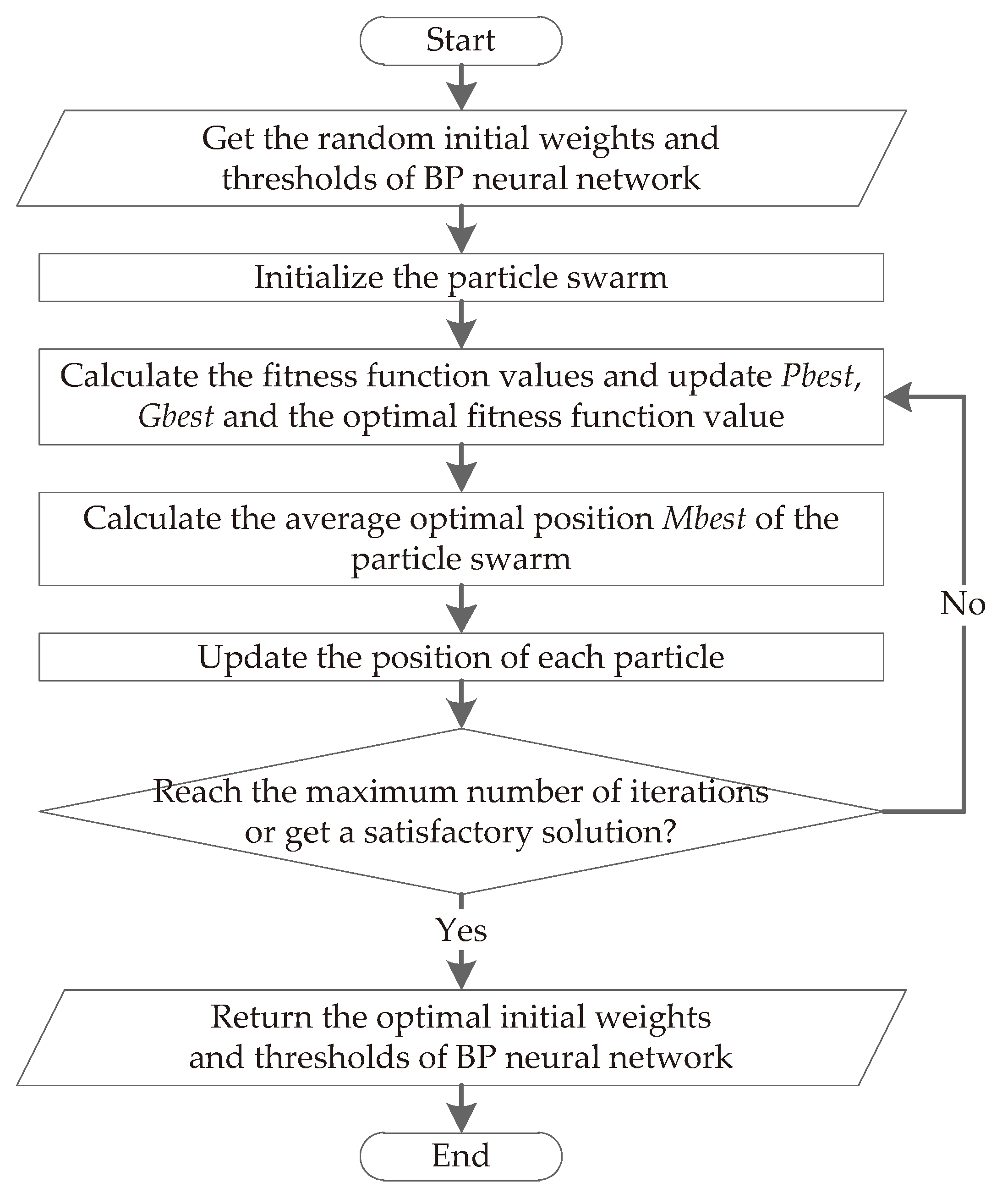
Due to the initializations of the weights and thresholds of the standard BP neural network are random, it is easy to fall into a local optimal solution during the training process, which makes it difficult to obtain an optimal neural network model. Therefore, the QPSO algorithm is introduced to find the optimal initial weights and thresholds to improve the convergence speed and fault prediction accuracy of BP neural network. The process of finding the optimal initial weights and thresholds using the QPSO algorithm is shown in Figure 3.

Step 1:

Obtain the initial weights and thresholds randomly selected by the BP neural network.

Step 2:

Initialize the particle swarm, including the setting of parameters such as swarm size and so on; the random generation of the initial position of each particle; the initial values of $P_{best}$ and $G_{best}$, and the fitness function value are set to 0, respectively, where $P_{best}$ denotes the historical optimal position of each particle and $G_{best}$ denotes the global optimal position of the particle swarm.

Step 3:

Calculate the current fitness function value of each particle, and update $P_{best}$, $G_{best}$ and the optimal fitness function value of the current particle swarm by comparing the results of the previous iteration and the current iteration

Step 4:

Calculate the average optimal position $M_{best}$ of the particle swarm, as shown in Equation (9), where M represents the swarm size and $P_{best.i}$ represents the historical optimal position of the i-th particle in the current iteration.

$$M_{best}=\frac{1}{M}\sum _{i=1}^M{P}_{best.i}$$

(9)

Step 5:

Update the position of each particle, as shown in Equation (10), where $x_i$ represents the position of the i-th particle, $\phi$ and u are uniformly distributed on (0, 1), $\alpha$ represents the shrinkage factor, and the probabilities of taking + and − is 50%, respectively.

$$x_i=\phi ·P_{best.i}+(1-\phi )G_{best}\pm \alpha \left|M_{best}-x_i\right|ln\left(\frac{1}{u}\right)$$

(10)

Step 6:

Determine whether the maximum number of iterations is reached or a satisfactory solution is obtained, if so, the optimal initial weights and thresholds is returned to the BP neural network; otherwise, go to Step 3.

3.6. Fusion of QPSO-BP Neural Network and Dempster–Shafer Evidence Theory

At first, the three QPSO-BP neural networks of the base end, drive end, and fan end are trained, respectively, to get the fault prediction results. Then, the prediction result of each sample (i.e., an eigenvector) is compared to the real state of that to get the corresponding confusion matrix, as shown in Equation (11).

$$C{M}_a=\left[\begin{array}{cccc}c{m}_{11}\hfill & c{m}_{12}\hfill & c{m}_{13}\hfill & c{m}_{14}\hfill \\ c{m}_{21}\hfill & c{m}_{22}\hfill & c{m}_{23}\hfill & c{m}_{24}\hfill \\ c{m}_{31}\hfill & c{m}_{32}\hfill & c{m}_{33}\hfill & c{m}_{34}\hfill \\ c{m}_{41}\hfill & c{m}_{42}\hfill & c{m}_{43}\hfill & c{m}_{44}\hfill \end{array}\right]$$

(11)

For brevity, the subscript a can be taken as 1, 2, and 3, representing the base end, drive end, and fan end, respectively. For example, $C{M}_1$ denotes the confusion matrix of the base end. In Equation (11), the row subscript and column subscript represent the real state and prediction result of the sample, respectively, and $c{m}_{ij}$ represents the ratio between the number of samples, which in real state i are judged as state j by the neural network, and the total number of samples, which are in real state i. The confusion matrix shows the prediction effect of the neural network.

According to the confusion matrix, the local reliability of the neural network model ${\omega }_{aj}$ can be calculated using Equation (12), and the global reliability of the neural network model ${\gamma }_a$ can be calculated using Equation (13).

$${\omega }_{aj}=c{m}_{jj}/\sum _{i=1}^{n}c{m}_{ij}$$

(12)

$${\gamma }_a=\frac{1}{n}\sum _{j=1}^n{\omega }_{aj}$$

(13)

The confusion matrices and local reliability of the base end, drive end, and fan end are shown in

Table 2. Confusion matrix and local reliability of the base end.

Real State	Prediction Results of the Base End
	Normal State	Inner Race Fault	Ball Fault	Outer Race Fault
Normal state	0.0000	0.0000	0.0000	0.0000
Inner race fault	0.0000	1.0000	0.0000	0.0000
Ball fault	0.0000	0.0014	0.9962	0.0024
Outer race fault	0.0000	0.0017	0.0000	0.9983
Local reliability	0.0000	0.9969	1.0000	0.9976

,

Table 3. Confusion matrix and local reliability of the drive end.

Real State	Prediction Results of the Drive End
	Normal State	Inner Race Fault	Ball Fault	Outer Race Fault
Normal state	1.0000	0.0000	0.0000	0.0000
Inner race fault	0.0011	0.9540	0.0333	0.0115
Ball fault	0.0000	0.0500	0.8430	0.1070
Outer race fault	0.0000	0.0102	0.0899	0.8999
Local reliability	0.9989	0.9406	0.8725	0.8836

and

Table 4. Confusion matrix and local reliability of the fan end.

Real State	Prediction Results of the fan End
	Normal State	Inner Race Fault	Ball fault	Outer Race Fault
Normal state	1.0000	0.0000	0.0000	0.0000
Inner race fault	0.0000	0.9860	0.0091	0.0049
Ball fault	0.0006	0.0144	0.9301	0.0549
Outer race fault	0.0020	0.0201	0.0173	0.9606
Local reliability	0.9974	0.9662	0.9724	0.9414

, respectively, and the global reliability obtained from the local reliability of the base end, drive end, and fan end is shown in

Table 5. Global reliability of the base end, drive end, and fan end.

Category	Local Reliability				Global Reliability
	Normal State	Inner Race Fault	Ball Fault	Outer Race Fault
Base end	0.0000	0.9969	1.0000	0.9976	0.9982
Drive end	0.9989	0.9406	0.8725	0.8836	0.9239
Fan end	0.9974	0.9662	0.9724	0.9414	0.9694

.

The weighted fusion and normalization are performed on the local reliability of the base end, drive end, and fan end and the posterior probability output $p_{aj}$, as shown in Equation (14).

$$p_{aj}^{\prime }={\omega }_{aj}{p}_{aj}/\sum _{j=1}^4{\omega }_{aj}{p}_{aj}$$

(14)

The basic probability distribution function can be defined according to the local reliability and global reliability of the base end, drive end, and fan end, as shown in Equation (15), where $\Omega$ denotes the uncertain set, and $A_1$, $A_2$, $A_3$, and $A_4$ represent the normal state, inner race fault, ball fault, and outer race fault of rolling bearing, respectively.

$$m_a\left(A_1,A_2,A_3,A_4,\Omega \right)=\left({\gamma }_a{p}_{a1}^{\prime },{\gamma }_a{p}_{a2}^{\prime },{\gamma }_a{p}_{a3}^{\prime },{\gamma }_a{p}_{a4}^{\prime },1-{\gamma }_a\right)$$

(15)

According to the Dempster combination rule, the final fault prediction result can be obtained using Equations (4)–(6).

4. Experimental Results and Analysis

4.1. Experimental Setup

The proposed rolling bearing fault prediction method based on QPSO-BP neural network and Dempster–Shafer evidence theory is implemented in MATLAB R2018a platform and tested on a computer with a hexa-core Intel i7-8750H CPU at 2.2 GHz and 16 GB RAM. The setting of parameters used in the training of BP neural network is listed in

Table 6. Parameters setting of BP neural network.

Parameter Name	Parameter Value
Transfer function	tansig
Learning function	learngdm
Learning rate	0.003
Momentum constant	0.9
Training function	Levenberg–Marquardt
Performance function	Mean Square Error
Error goal	0.0001
Number of iterations	1000

.

The transfer function is used to calculate the output of a neuron based on its input. The commonly used transfer functions include log-sigmoid, tan-sigmoid, poslin, purelin, radbas, and tribas, where tan-sigmoid is the best selection in our experiments. The tan-sigmoid function can smoothly map the real number field to the interval [0, 1], and it is monotonically increasing and continuously derivable. It is shown in Equation (16), where n is the input of a neuron and e is the Euler number.

$$tansig\left(n\right)=\frac{2}{1+e^{-2n}}-1$$

(16)

The learning function is used to calculate the change of weights of BP neural network. Learngdm is the gradient descent with momentum weights learning function, which can be described as

$$dW=mc\ast d{W}_{prev}+(1-mc)\ast lr\ast gW$$

(17)

where $dW$ represents the weight change of a neuron, $d{W}_{prev}$ represents the previous $dW$, $mc$ represents the momentum constant and is set to 0.9, $lr$ represents the learning rate and is set to 0.003, and $gW$ represents the previous gradient of weight change. The training function is used to update weights and thresholds, and the Levenberg–Marquardt algorithm [32] is selected in our experiments, because it can effectively solve the nonlinear least squares problem and is one of the most efficient backpropagation algorithms. The Levenberg–Marquardt algorithm has the advantages of both gradient method and Newton method and can be described as

$$x_{k+1}=x_k-\frac{J^{\mathrm{T}}e}{J^{\mathrm{T}}J+\mu I}$$

(18)

where $x_k$ represents the weights and thresholds of the k-th iteration, J represents the Jacobian matrix that contains first derivatives of the network errors with respect to the weights and biases, I represents the identity matrix, e represents the vector of network errors, and $\mu$ is the step size for gradient descent. When the descent is fast, the small $\mu$ is used to make the equation close to Newton method, and when the descent is slow, the large $\mu$ is used to make the equation close to gradient method. The performance function is used to measure the performance of neural network, and the mean square error (MSE) is adopted in our experiments. The MSE can be calculated using Equation (19), where n is the number of weights and thresholds to be optimized, and $Y_i$ and ${\widehat{Y}}_i$ denote the observed value and predicted value of the i-th variable, respectively. The value of the performance function can always be reduced after each iteration, and when the number of iterations reaches 1000 or the error value is less than 0.0001, the iteration ends.

$$\mathrm{MSE}=\frac{1}{n}\sum _{i=1}^n{\left(Y_i-{\widehat{Y}}_i\right)}^2$$

(19)

The parameters setting of QPSO algorithm used to find the optimal initial weights and thresholds is listed in

Table 7. Parameters setting of QPSO algorithm.

Parameter Name	Parameter Value
Shrinkage factor	0.8
Dimension of particles	160
Number of particles	100
Error goal	0.001
Number of iterations	1000

. The shrinkage factor is used to control the convergence speed of QPSO algorithm and is set to 0.8. The dimension of particles is the sum of the number of weights and thresholds from input-layer to hidden-layer and the number of weights and thresholds from hidden-layer to output-layer, which can be calculated using Equation (20), where x, h, and y are the number of neurons in the input-layer, hidden-layer, and output-layer, respectively. The number of particles is set to 100, which means that 100 random solutions are first initialized and then the optimal solutions are searched iteratively. When the number of iterations reaches 1000 or the error value is less than 0.001, the iteration ends.

$$dimP=(x\ast h+h)+(h\ast y+y)$$

(20)

4.2. Analysis of Selecting the Optimal Number of Hidden-Layer Nodes

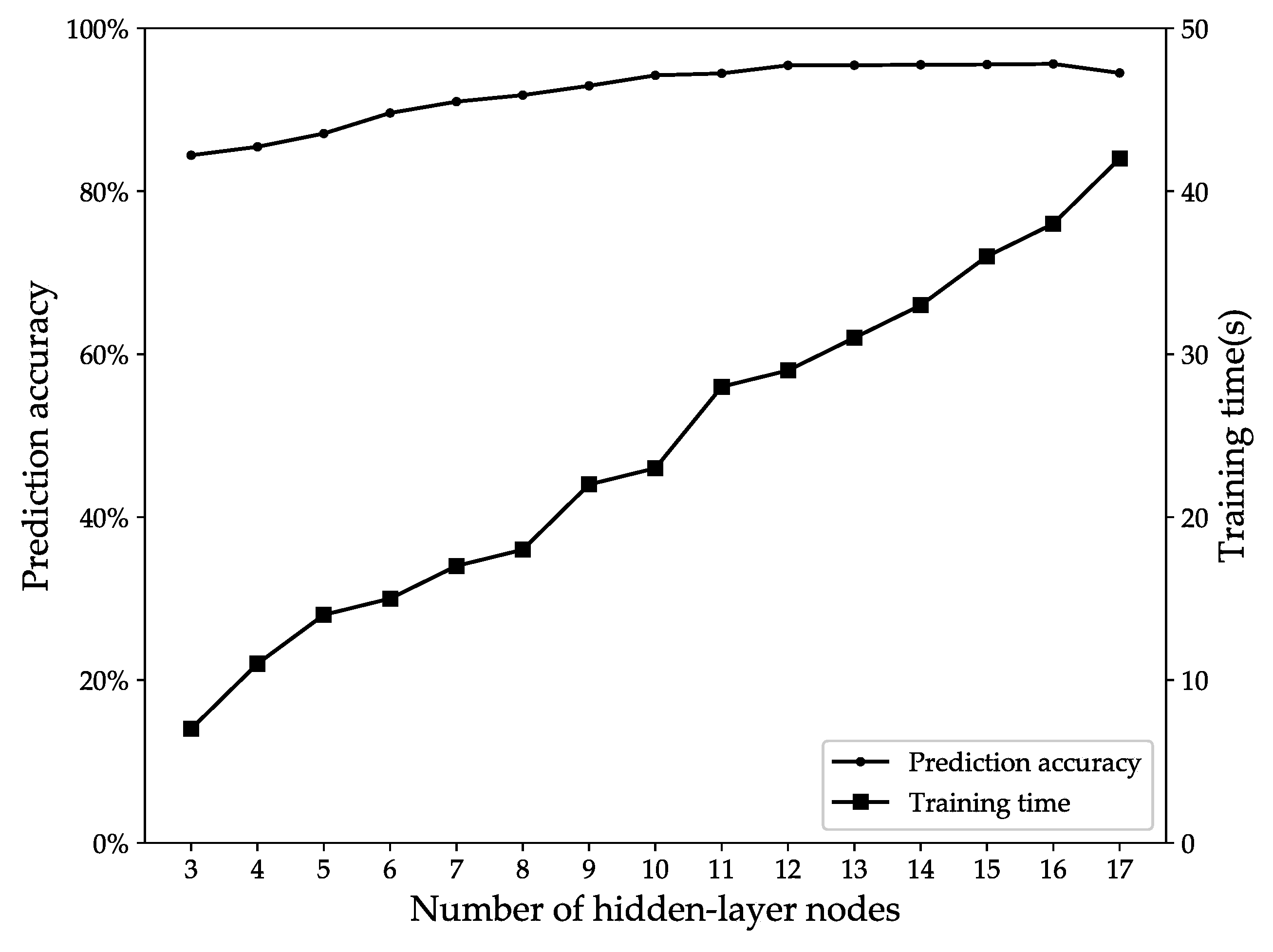
To verify the effectiveness of finding the optimal number of hidden-layer nodes by using the dichotomy method, first, the lower bound and upper bound of the number of hidden-layer nodes are taken as 3 and 17, respectively, according to Equations (7) and (8). Second, the step-by-step method is used to manually find the optimal number of hidden-layer nodes. Third, the dichotomy method is used to automatically find the optimal number of hidden-layer nodes. The experimental results are presented in Figure 4 and Figure 5.

Figure 4 presents the influence of different number of hidden-layer nodes on the fault prediction accuracy and training time with the step-by-step method. When the fault prediction accuracy and training time are taken into consideration, after completing 15 searches in 364 s, the optimal number of hidden-layer nodes is determined as 12 by using the evaluation index E adopted in Algorithm 1. Figure 5 presents the process of finding the optimal number of hidden-layer nodes using the dichotomy method. After completing 6 searches in 163 s, the optimal number of hidden-layer nodes is also determined as 12. The results indicate that the step-by-step method is time-consuming and labor-intensive, and it is difficult to obtain the optimal number of hidden-layer nodes for large-scale neural network. However, the proposed dichotomy method can significantly improve the efficiency of selecting the optimal number of hidden-layer nodes, when the number of hidden-layer nodes h is large, the number of searches can be reduced from h to ${log}_{2}h$ in theory, and the search time can also be reduced greatly.

4.3. Prediction Results of Rolling Bearing Fault Under Different Working Conditions

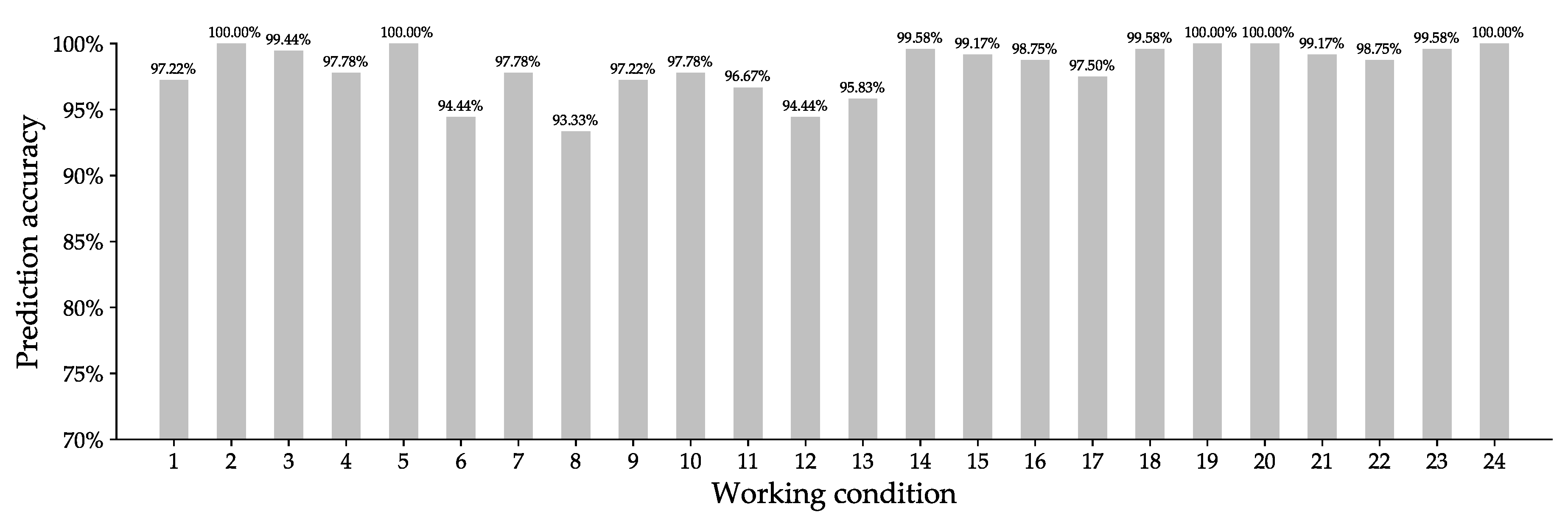
To evaluate the effectiveness of the rolling bearing fault prediction method proposed in this paper, the test set is used to verify the proposed rolling bearing fault prediction model QPSO-BP-DS. The prediction accuracy of different types of rolling bearing fault under 24 different working conditions listed in

Table 8. Different working conditions.

Working Condition	Sampling Frequency (kHz)	Fault Diameter (inch)	Motor Load (HP)
1	12	0.007	0
2	12	0.007	1
3	12	0.007	2
4	12	0.007	3
5	12	0.014	0
6	12	0.014	1
7	12	0.014	2
8	12	0.014	3
9	12	0.021	0
10	12	0.021	1
11	12	0.021	2
12	12	0.021	3
13	48	0.007	0
14	48	0.007	1
15	48	0.007	2
16	48	0.007	3
17	48	0.014	0
18	48	0.014	1
19	48	0.014	2
20	48	0.014	3
21	48	0.021	0
22	48	0.021	1
23	48	0.021	2
24	48	0.021	3

are shown in Figure 6, Figure 7 and Figure 8.

Figure 6, Figure 7 and Figure 8 show that the proposed method can effectively predict different types of rolling bearing fault under different working conditions; the average prediction accuracy of the inner race fault, ball fault, and outer race fault can reach 98.52%, 98.65%, and 98.60%, respectively, and the overall average prediction accuracy can reach 98.59%. It is not difficult to see that the prediction results of the inner race fault and ball fault are more stable than that of the outer race fault, which may be because the outer race fault has a greater impact on the performance of rotating machinery under some working conditions, and the vibration data obtained under those working conditions fluctuates greatly. The results also show that the proposed rolling bearing fault prediction model has good generalization ability, which is mainly due to the initial weights and thresholds of BP neural network are optimized by the QPSO algorithm and the fault classification results of three QPSO-BP neural networks are fused by Dempster–Shafer evidence theory.

To further evaluate the generalization ability of the proposed rolling bearing fault prediction model, the dataset composed of eigenvectors is divided into the training set and test set according to seven different ratios (i.e., 3:7, 4:6, 5:5, 6:4, 7:3, 8:2, and 9:1). Figure 9 presents the average prediction accuracy of rolling bearing fault obtained under different ratios of training set to test set. When the proportion of training set increases from 30% to 60%, the average prediction accuracy of rolling bearing fault has been growing rapidly and increases from 75.73% to 96.18%. If the proportion of training set is too small, the neural network may not obtain a good mapping relationship from the fault features to the accurate classification results through the training set, thereby causing the problem of overfitting. After the proportion of training set reaches 60%, the prediction accuracy has been growing slowly. When the proportion of training set is 90%, the average prediction accuracy reaches up to 98.59%. The results further prove the proposed fault prediction model has strong generalization ability.

4.4. Analysis of the Fusion Effect of Dempster–Shafer Evidence Theory

To verify the effectiveness of Dempster–Shafer evidence theory used in improving the prediction accuracy of rolling bearing fault, first the test sets of the base end, drive end, and fan end are used to test the fault prediction models of the base end (QPSO-BP-BA), drive end (QPSO-BP-DE), and fan end (QPSO-BP-FE), respectively, and then all the test sets are used to test the proposed fault prediction model (QPSO-BP-DS). The prediction results of different fault prediction models are shown in

Table 9. Prediction results of different fault prediction models.

Fault Prediction Model	Average Prediction Accuracy
QPSO-BP-BA	99.39%
QPSO-BP-DE	91.30%
QPSO-BP-FE	95.91%
QPSO-BP-DS	98.59%

.

As can be seen from Table 9, the average prediction accuracy obtained by QPSO-BP-DS is higher than that obtained by QPSO-BP-DE or QPSO-BP-FE, but is lower than that obtained by QPSO-BP-BA. This is primarily because the training set and test set of the base end are small, and the vibration data collected by the sensor deployed on the base end only contains the inner race fault data, ball fault data, and outer race fault data under 12K sampling frequency, but the normal data under 12K sampling frequency and all the data under 48K sampling frequency are missing. QPSO-BP-BA can obtain a higher prediction accuracy for the test set of the base end, but the prediction accuracy will decline for the test sets of the drive end and fan end. Therefore, QPSO-BP-BA cannot predict the rolling bearing fault comprehensively. This problem can be effectively solved by using Dempster–Shafer evidence theory to fuse the fault classification results of the three QPSO-BP neural networks of the base end, drive end, and fan end.

To further illustrate the effectiveness of Dempster–Shafer evidence theory used in improving the fault prediction accuracy, one sample is selected for testing.

Table 10. Prediction results of a test sample.

Fault Prediction Model	Reliability Function Value					Prediction Result
	$\mathit{m}\left({\mathit{A}}_{\mathbf{1}}\right)$	$\mathit{m}\left({\mathit{A}}_{\mathbf{2}}\right)$	$\mathit{m}\left({\mathit{A}}_{\mathbf{3}}\right)$	$\mathit{m}\left({\mathit{A}}_{\mathbf{4}}\right)$	$\mathit{m}(\Omega )$
QPSO-BP-BA	0.0000	0.4814	0.1229	0.2455	0.1502	$A_2$
QPSO-BP-DE	0.1208	0.2026	0.0387	0.4427	0.1952	$A_4$
QPSO-BP-FE	0.0434	0.7633	0.0192	0.0792	0.0949	$A_2$
QPSO-BP-DS	0.0143	0.8029	0.0170	0.1553	0.0105	$A_2$

presents the prediction results of a test sample with different fault prediction models. As shown in Table 10, the real state of this sample is the inner race fault, and the prediction results obtained by QPSO-BP-BA, QPSO-BP-DE, QPSO-BP-FE, and QPSO-BP-DS are the inner race fault, outer race fault, inner race fault, and inner race fault, respectively. The results show that the most reliable prediction result can be obtained by the Dempster synthesis rule when the prediction results of the three QPSO-BP neural networks are not consistent. Therefore, the fusion of QPSO-BP neural network and Dempster–Shafer evidence theory can effectively reduce misdiagnosis and improve the fault prediction accuracy.

4.5. Analysis of the Optimization Effect of QPSO Algorithm

To better evaluate the optimization effect of QPSO algorithm on BP neural network, the other five different metaheuristic optimization algorithms, including GA [21], DE [22], PSO [23], GSO [24], and ISFLA [25], are also used for optimizing the initial weights and thresholds. In this experiment, first, the same training set is used to train the BP neural network without optimization and the other BP neural networks optimized by different algorithms (i.e., GA, DE, PSO, GSO, ISFLA, and QPSO). Note that these BP neural networks have the same training parameters listed in Table 6 and network structures shown in Figure 2, so as to make a fair comparison. Second, Dempster–Shafer evidence theory is combined with these BP neural networks to obtain seven different rolling bearing fault prediction models (i.e., BP-DS, GA-BP-DS, DE-BP-DS, PSO-BP-DS, GSO-BP-DS, ISFLA-BP-DS, and QPSO-BP-DS). Finally, the same test set is used to verify the seven fault prediction models. The setting of key parameters used in different optimization algorithms are as follows.

• GA: the population size is set to 100, the mutation probability is set to 0.2, and the crossover probability is set to 0.5.
• DE: the population size is set to 100, the differential weight is set to 1.2, and the crossover probability is set to 0.5.
• PSO: the number of particles is set to 100, the initial and end inertia weights are set to 0.9 and 0.4, the cognition acceleration factor is set to 0.73, and the social acceleration factor is set to 2.05.
• GSO: the number of glowworms is set to 100, the shrink factor is set to 0.2, the maximum attractiveness is set to 1, and the absorption coefficient is set to 1.
• ISFLA: the convergence factor is set to 0.8, the memeplexes is set to 10, the number of frogs in each memeplex is set to 10, and the number of evolved frogs selected from each memeplex is set to 7.
• QPSO: see Table 7.

Table 11. Prediction results of fault prediction models with different optimization algorithms.

Fault Prediction Model	Average Prediction Accuracy
BP-DS	96.37%
GA-BP-DS	96.92%
DE-BP-DS	97.01%
PSO-BP-DS	97.12%
GSO-BP-DS	97.32%
ISFLA-BP-DS	97.68%
The proposed QPSO-BP-DS	98.59%

presents the prediction results of fault prediction models with different optimization algorithms. The average prediction accuracy of BP-DS, GA-BP-DS, DE-BP-DS, PSO-BP-DS, GSO-BP-DS, ISFLA-BP-DS, and QPSO-BP-DS are 96.37%, 96.92%, 97.01%,97.12%, 97.32%, 97.68%, and 98.59%, respectively. Obviously, the BP neural networks with different optimization algorithms perform better than the BP neural network without optimization. The GA has a definite theoretical basis and is easy to understand, but facing the massive weights and thresholds needed to be optimized, it is easy to fall into the local optimal and has lower efficiency in the later stage of evolution. The DE algorithm is similar to GA, it is easier to implement, and has faster convergence speed than GA, but it easily produces premature convergence with the reduction of diversity of the population. The PSO algorithm has the advantages of fast convergence and strong global optimization capability, but it needs to control three parameters including inertia weight, cognition acceleration factor, and social acceleration factor, the tuning of these parameters has a great effect on the optimization performance of PSO algorithm, and it is often difficult to find a group of the best parameters. Both GSO algorithm and ISFLA are novel swarm intelligence optimization algorithms, the GSO algorithm has strong local search ability, but it converges slowly at later period and is easy to relapse into premature convergence and local best. The ISFLA introduces the convergence factor and chaotic operator to overcome shortcomings of shuffled frog leaping algorithm, and it has high solution accuracy and fast convergence.

Compared with GA-BP-DS, DE-BP-DS, PSO-BP-DS, GSO-BP-DS, and ISFLA-BP-DS, the proposed QPSO-BP-DS achieves higher fault prediction accuracy; this is mainly because the optimal initial weights and thresholds used in QPSO-BP-DS are found by QPSO algorithm with stronger global optimization ability. In addition, the QPSO algorithm only needs to control the shrinkage factor, so it more easily obtains the global optimal solution.

4.6. Comparison with Other Fault Classifiers Based on Machine Learning

To further verify the effectiveness of the proposed rolling bearing fault prediction method, the proposed QPSO-BP neural network is compared with the other five different classifiers including SVM [2], DT [3], RF [4], k-NN [5], and K-Means [6]. In this experiment, first, the same training set is used to train the fault classifiers based on different methods (i.e., SVM, DT, RF, k-NN, K-Means, and QPSO-BP neural network). Second, Dempster–Shafer evidence theory is combined with these fault classifiers to obtain six different rolling bearing fault prediction models (i.e., SVM-DS, DT-DS, RF-DS, k-NN-DS, K-Means-DS, and QPSO-BP-DS). Finally, the same test set is used to verify the six fault prediction models. The setting of key parameters used in different classifiers are as follows.

• SVM: the radial basis function (RBF) is taken as the kernel function, the penalty parameter C of error term is set to 1, and the parameter $\gamma$ is set to 0.125.
• DT: the maximum depth of the decision tree is set to 5 and ‘$entropy$’ is taken as the feature selection criterion.
• RF: the number of sub-trees is set to 100 and the maximum number of features used by a single decision tree is set to 3.
• k-NN: the number of neighbors is set to 5 and ‘$uniform$’ is taken as the weights.
• K-Means: the number of clusters is set to 4 and the number of iterations is set to 1000.
• QPSO-BP neural network: see Table 6 and Table 7.

Table 12. Comparison with different fault classifiers based on machine learning.

Fault Prediction Model	Average Prediction Accuracy	Macro F1-Score	Macro AUC
SVM-DS	95.20%	96.31%	0.9645
DT-DS	93.42%	93.76%	0.9452
RF-DS	95.63%	97.02%	0.9673
k-NN-DS	92.87%	93.60%	0.9405
K-Means-DS	92.18%	93.55%	0.9233
The proposed QPSO-BP-DS	98.59%	98.80%	0.9858

presents the prediction results of fault prediction models with different classifiers using three different evaluation criteria. The accuracy is used to evaluate the overall performance of fault classifier, the macro F1-score is used to evaluate the performance of fault classifier by comprehensively considering the precision and recall rate, and the macro AUCis used to evaluate the prediction effect of fault classifier according to the probability that the score of any positive instances is greater than the score of any negative instances. It is easy to see that the proposed QPSO-BP neural network provides higher fault prediction accuracy, macro F1-score, and macro AUC than the other classifiers. The training set and test set used in this experiment have the characteristics of huge amount of data and various and complex fault. The strategy of combining multiple support vector machines in multi-classification problem has a great influence on the fault classification results of SVM-DS. The method of layer-by-layer reasoning in decision tree can easily lead to overfitting and affect the fault classification accuracy of DT-DS. The same fault feature of rolling bearing has the characteristics of multi-level division in random forest, which could affect the classification accuracy of RF-DS. Due to the vibration data obtained under 24 different working conditions are nonuniformly distributed, which will affect the average prediction accuracy of k-NN-DS. The prediction effect of K-Means-DS is sensitivity to the initial clustering centers, and the misclassification data would affect the clustering centers during iteration. Compared with SVM, DT, RF, k-NN, and K-Means, the proposed QPSO-BP neural network is superior in dealing with the complicated vibration data obtained under different working conditions.

4.7. Comparison with Other Fault Classifiers Based on Deep Learning

To further evaluate the effectiveness of the proposed method, the comparisons with the other four different fault classifiers based on deep learning are conducted, including VI-CNN [11], AlexNet [12], VGG-19 [13], and ResNet-50 [14]. The CWRU dataset is still used in this experiment. During the preprocessing of experimental data, all the original one-dimensional vibration data are transformed to two-dimensional gray images, and the transformation process is as follows; (i) every 4096 pieces of continuous data are divided into a sample; (ii) all the data of each sample are normalized to the range [0, 255]; and (iii) each sample is divided into 64 equal parts, which are aligned as the rows of the two-dimensional gray image of 64 × 64 pixels. After the preprocessing, 1980 gray images of the base end, 6110 gray images of the drive end, and 6110 gray images of the fan end are obtained finally. These gray images are used as input data of VI-CNN, AlexNet, VGG-19, and ResNet-50, and they are divided into training set and test set according to the ratio of 9:1. The settings of network structure and hyperparameters of VI-CNN, AlexNet, VGG-19, and ResNet-50 can be found in [11,33,34,35], respectively. As for these CNN models, the gray images of 64 × 64 pixels are used in the input layer, and the output layer uses four neurons to classify the gray images into four different categories corresponding to the normal state, inner race fault, ball fault, and outer race fault of rolling bearing.

Table 13. Comparison with different fault classifiers based on deep learning.

Fault Prediction Model	Average Prediction Accuracy	Training Time (s)	Model Size (MB)
VI-CNN	96.60%	496	0.26
AlexNet	99.01%	903	77.48
VGG-19	99.07%	1317	188.06
ResNet-50	99.18%	2559	90.25
The proposed QPSO-BP-DS	98.59%	87	0.02

shows the average prediction accuracy, training time, and model size of different fault prediction models. The average prediction accuracy of the proposed QPSO-BP-DS is 1.99% higher than that of VI-CNN, and the training time of VI-CNN is 5.70× as long as that of the proposed QPSO-BP-DS, which shows that the proposed QPSO-BP-DS achieves better performance than VI-CNN in rolling bearing fault prediction. The average prediction accuracy of the proposed QPSO-BP-DS is 0.42%, 0.48%, and 0.59% lower than that of AlexNet, VGG-19, and ResNet-50, respectively, but the training time of the proposed QPSO-BP-DS is decreased by 90.37%, 93.39%, and 96.60% than that of AlexNet, VGG-19, and ResNet-50, respectively. AlexNet, VGG-19, and ResNet-50 have more complicated network structures than the proposed QPSO-BP, they utilize deeper neural network to learn and extract fault features of rolling bearing, which is helpful to improve fault prediction accuracy. However, the more complex the network structure, the more complex the computation and the longer the training time. Note from the experimental comparison that the proposed QPSO-BP-DS not only has better fault prediction accuracy but also has less training time.

4.8. Comparison with Ensemble Classifier

Ensemble learning is a research hotspot in the machine learning field, and its purpose is to build an ensemble classifier with better classification accuracy and stronger generalization ability using multiple homogeneous or heterogeneous base classifiers. Lei et al. [36] proposed an ensemble approach based on ant colony optimization and rough set for efficiently and effectively classifying biomedical data, which can decrease ensemble size and improve classification performance by selecting a subset of all trained base classifiers in ensemble learning. Abdolrahman et al. [37] proposed an ensemble method based on multi-objective PSO algorithm for power transformers fault diagnosis, which can improve diagnosis accuracy by finding the best subset of features and the best group of classifiers. Md. Jan et al. [38,39,40] proposed an ensemble classifier generation framework for generating an ensemble classifier that can achieve higher classification accuracy with lower ensemble size by incorporating a multi-constrained PSO algorithm, and the experimental results show that it outperforms the state-of-the-art ensemble classifier approaches. In this paper, an ensemble classifier for rolling bearing fault prediction is implemented according to [38,39,40], and four base classifiers (SVM, DT, k-NN, and the proposed QPSO-BP) are used in the training process of the ensemble classifier.

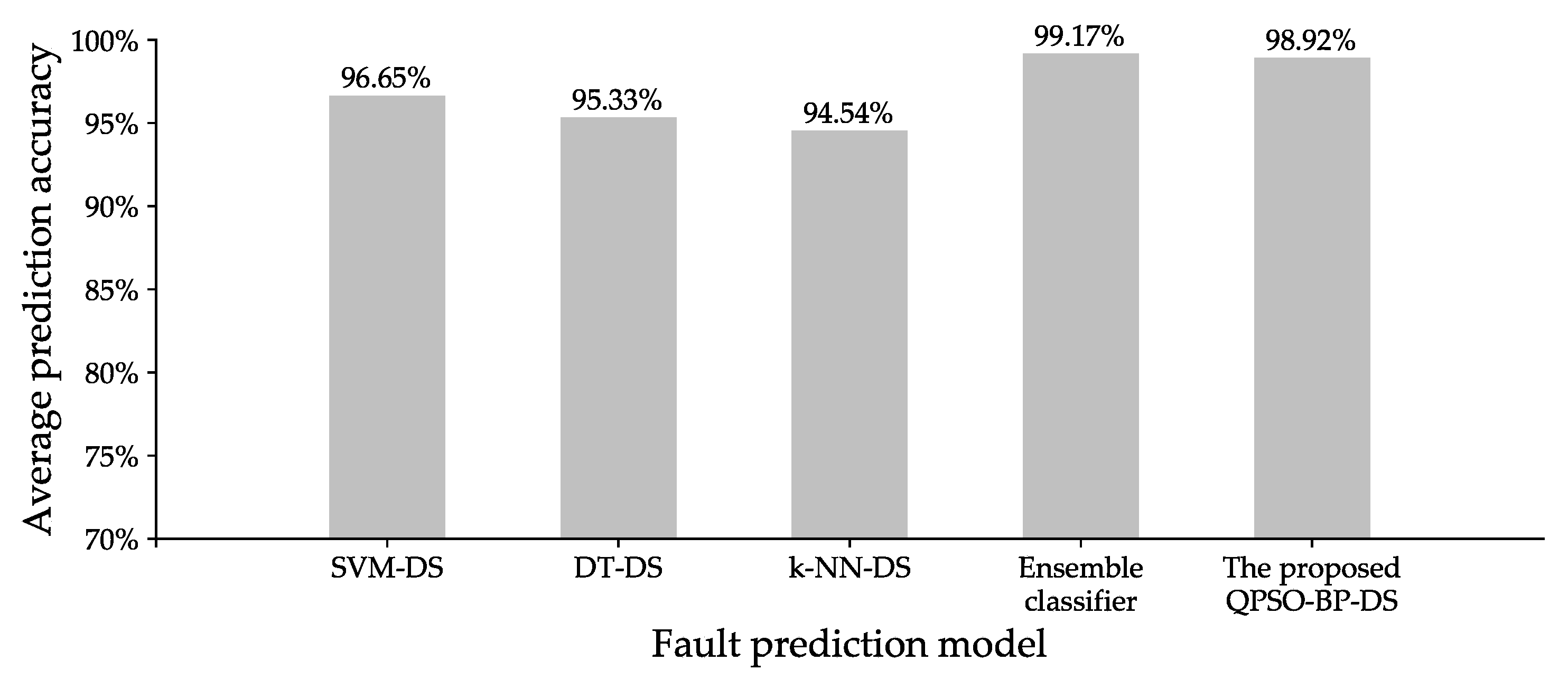
In this subsection, a new rolling bearing fault dataset from the Society for Machinery Failure Prevention Technology (MFPT) [41] is introduced, which has ~5.6 million pieces of vibration data under different motor loads, including three kinds of normal state data, seven kinds of inner race fault data, and ten kinds of outer race fault data. According to the preprocessing method described in Section 3.2, first, every 2000 pieces of vibration data are divided into a sample; then three-layer wavelet packet decomposition is used to obtain 879 groups of normal state eigenvectors, 1390 groups of outer race fault eigenvectors, and 511 groups of inner race fault eigenvectors; and finally the dataset composed of eigenvectors is divided into training set and test set according to the ratio of 9:1.

In this experiment, the performance comparison among SVM-DS, DT-DS, k-NN-DS, ensemble classifier, and the proposed QPSO-BP-DS is conducted on MFPT dataset. The setting of key parameters used in SVM-DS, DT-DS, k-NN-DS, and the proposed QPSO-BP-DS can be found in Section 4.6, and the following two changes need to be made; the number of output-layer nodes of QPSO-BP is set to 3 and the dimension of particles of QPSO is set to 147. The setting of main parameters used in the ensemble classifier is as follows.

• Base classifiers: the kernel function of SVM is RBF, the leaf size of DT is a random number between 3 and 30, the number of nearest neighbors of k-NN is a random number between 1 and 10, and the number of hidden-layer nodes of QPSO-BP is a random number between 3 and 17.
• The maximum number of data clusters K is set to 14 and the number of iterations of K-Means is set to 2000.
• The binary threshold $\theta$ of PSO algorithm is set to 0.6 and the number of iterations of PSO algorithm is set to 1000.

As shown in Figure 10, the average prediction accuracy of the proposed QPSO-BP-DS is 2.27%, 3.59%, and 4.38% higher than that of SVM-DS, DT-DS, and k-NN-DS, respectively. The results show that the proposed method achieves good performance on different dataset; this further confirms that the proposed method has strong generalization ability. Note from Figure 10 that the average prediction accuracy of the proposed QPSO-BP-DS is 0.25% lower than that of ensemble classifier because the ensemble classifier can maximize the classification accuracy of each base classifier by incorporating PSO algorithm [38]. However, the computation of ensemble classifier is more complicated than that of the proposed QPSO-BP-DS; this means that the ensemble classifier need more time to train.

5. Conclusions

In this paper, a rolling bearing fault prediction method based on QPSO-BP neural network and Dempster–Shafer evidence theory is proposed, and it is verified by the rolling bearing dataset from CWRU. The three-layer wavelet packet decomposition is used to analyze the original vibration data collected on the base end, drive end, and fan end of rolling bearing, and the eigenvectors of different states of rolling bearing are obtained. The dichotomy method is used to find the optimal number of hidden-layer nodes of BP neural network automatically, compared with the manual step-by-step testing method, it greatly improves the efficiency of selecting the optimal number of hidden-layer nodes. The QPSO algorithm is used to optimize the initial weights and thresholds of BP neural network, and the optimal initial weights and thresholds are found, which not only improves the convergence speed of BP neural network, but also improves the fault prediction accuracy. Compared with the BP neural network without optimization, the average accuracy of rolling bearing fault prediction based on QPSO-BP neural network is increased by 2.22%. Dempster–Shafer evidence theory is used to fuse the fault classification results of three QPSO-BP neural networks of the base end, drive end, and fan end to obtain the final rolling bearing fault prediction model; the experimental results show that it can effectively predict different types of rolling bearing fault under various working conditions.

In the actual industrial production environment, the scale of rolling bearing data is increasingly large and the data acquisition is often accompanied by a strong noise, in the future work, the parallelization and optimization of rolling bearing fault prediction model based on distributed computing platform will be explored.

References

- Li, C.; De Oliveira, J.V.; Cerrada, M.; Cabrera, D.; Sánchez, R.V.; Zurita, G. A systematic review of fuzzy formalisms for bearing fault diagnosis. IEEE Trans. Fuzzy Syst. 2019, 27, 1362–1382. [Google Scholar] [CrossRef]
- Chen, R.; Huang, D.; Zhao, L. Fault diagnosis of rolling bearing based on EEMD information entropy and improved SVM. In Proceedings of the IEEE Chinese Control Conference (CCC), Guangzhou, China, 27–30 July 2019; pp. 4961–4966. [Google Scholar] [CrossRef]
- Zhao, X.; Qin, Y.; Kou, L.; Liu, Z. Understanding real faults of axle box bearings based on vibration data using decision tree. In Proceedings of the IEEE International Conference on Prognostics and Health Management (ICPHM), Seattle, WA, USA, 11–13 June 2018; pp. 1–5. [Google Scholar] [CrossRef]
- Chen, Y.; Zhang, T.; Zhao, W.; Luo, Z.; Sun, K. Fault diagnosis of rolling bearing using multiscale amplitude-aware permutation entropy and random fores. Algorithms 2019, 12, 184. [Google Scholar] [CrossRef] [Green Version]
- Appana, D.K.; Islam, M.R.; Kim, J.M. Reliable fault diagnosis of bearings using distance and density similarity on an enhanced k-NN. In Proceedings of the Australasian Conference on Artificial Life and Computational Intelligence, Geelong, VIC, Australia, 31 January–2 February 2017; Springer: Berlin, Germany, 2017; pp. 193–203. [Google Scholar] [CrossRef]
- Shi, Z.; Song, W.; Taheri, S. Improved LMD, permutation entropy and optimized K-means to fault diagnosis for roller bearings. Entropy 2016, 18, 70. [Google Scholar] [CrossRef]
- Eren, L.; Ince, T.; Kiranyaz, S. A generic intelligent bearing fault diagnosis system using compact adaptive 1D CNN classifier. J. Signal Process. Syst. 2019, 91, 179–189. [Google Scholar] [CrossRef]
- Liang, P.; Deng, C.; Wu, J.; Yang, Z.; Zhu, J. Intelligent fault diagnosis of rolling element bearing based on convolutional neural network and frequency spectrograms. In Proceedings of the IEEE International Conference on Prognostics and Health Management (ICPHM), San Francisco, CA, USA, 17–20 June 2019; pp. 1–5. [Google Scholar] [CrossRef]
- Huang, T.; Fu, S.; Feng, H.; Kuang, J. Bearing fault diagnosis based on shallow multi-scale convolutional neural network with attention. Energies 2019, 12, 3937. [Google Scholar] [CrossRef] [Green Version]
- Liu, H.; Yao, D.; Yang, J.; Li, X. Lightweight convolutional neural network and its application in rolling bearing fault diagnosis under variable working conditions. Sensors 2019, 19, 4827. [Google Scholar] [CrossRef] [PubMed] [Green Version]
- Hoang, D.T.; Kang, H.J. Rolling element bearing fault diagnosis using convolutional neural network and vibration image. Cogn. Syst. Res. 2019, 53, 42–50. [Google Scholar] [CrossRef]
- Wen, L.; Li, X.; Gao, L.; Zhang, Y. A new convolutional neural network-based data-driven fault diagnosis method. IEEE Trans. Ind. Electron. 2017, 65, 5990–5998. [Google Scholar] [CrossRef]
- Wen, L.; Li, X.; Li, X.; Gao, L. A new transfer learning based on VGG-19 network for fault diagnosis. In Proceedings of the IEEE 23rd International Conference on Computer Supported Cooperative Work in Design (CSCWD), Porto, Portugal, 6–8 May 2019; pp. 205–209. [Google Scholar] [CrossRef]
- Wen, L.; Li, X.; Gao, L. A transfer convolutional neural network for fault diagnosis based on ResNet-50. Neural Comput. Appl. 2019, 1–14. [Google Scholar] [CrossRef]
- Sun, Y.; Gao, H.; Hong, X.; Song, H.; Liu, Q. Fault diagnosis for rolling bearing based on deep residual neural network. In Proceedings of the International Conference on Sensing, Diagnostics, Prognostics, and Control (SDPC), Xi’an, China, 15–17 August 2018; pp. 421–425. [Google Scholar] [CrossRef]
- Cui, Q.; Li, Z.; Yang, J.; Liang, B. Rolling bearing fault prognosis using recurrent neural network. In Proceedings of the IEEE 29th Chinese Control And Decision Conference (CCDC), Chongqing, China, 28–30 May 2017; pp. 1196–1201. [Google Scholar] [CrossRef]
- Lin, H.; Xinyue, Z.; Handong, L. Bearing fault diagnosis based on BP neural network. In Proceedings of the IOP Conference Series: Earth and Environmental Science, Hong Kong, China, 26–28 October 2018; IOP Publishing: Bristol, UK, 2018; Volume 208, p. 012092. [Google Scholar] [CrossRef]
- Song, M.; Song, H.; Xiao, S. A study on fault diagnosis method of rolling bearing based on wavelet packet and improved BP neural network. In IOP Conference Series: Materials Science and Engineering Conference Series; IOP Publishing: Bristol, UK, 2017; Volume 274, p. 012133. [Google Scholar] [CrossRef] [Green Version]
- Sharma, A.; Jigyasu, R.; Mathew, L.; Chatterji, S. Bearing fault diagnosis using frequency domain features and artificial neural networks. In Information and Communication Technology for Intelligent Systems; Springer: Berlin, Germany, 2019; pp. 539–547. [Google Scholar] [CrossRef]
- Zhang, R.; Fang, Y.; Zhou, Z. Fault diagnosis of rolling bearing based on k-svd dictionary learning algorithm and BP neural network. In Proceedings of the International Conference on Robotics, Intelligent Control and Artificial Intelligence, Shanghai, China, 20–22 September 2019; pp. 341–345. [Google Scholar] [CrossRef]
- Wen, Y.; Jia, M.; Luo, C. Study of fault diagnosis for rolling bearing based on GA-BP algorithm. In Proceedings of the 2nd International Conference on Automation, Mechanical Control and Computational Engineering (AMCCE 2017), Beijing, China, 25–26 March 2017; Atlantis Press: Beijing, China. [Google Scholar] [CrossRef] [Green Version]
- Shi, J.; Wu, X.; Zhou, J.; Wang, S. BP neural network based bearing fault diagnosis with differential evolution & EEMD denoise. In Proceedings of the IEEE 9th International Conference on Modelling, Identification and Control (ICMIC), Beijing, China, 10–12 July 2017; pp. 1038–1043. [Google Scholar] [CrossRef]
- Yuan, H.; Wang, X.; Sun, X.; Ju, Z. Compressive sensing-based feature extraction for bearing fault diagnosis using a heuristic neural network. Meas. Sci. Technol. 2017, 28, 065018. [Google Scholar] [CrossRef]
- Xu, Q.; Liu, Y.Q.; Tian, D.; Long, Q. Rolling bearing fault diagnosis method using glowworm swarm optimization and artificial neural network. In Advanced Materials Research; Trans Tech Publications: Zurich, Switzerland, 2014; Volume 860, pp. 1812–1815. [Google Scholar] [CrossRef]
- Zhao, Z.; Xu, Q.; Jia, M. Improved shuffled frog leaping algorithm-based BP neural network and its application in bearing early fault diagnosis. Neural Comput. Appl. 2016, 27, 375–385. [Google Scholar] [CrossRef]
- Case Western Reserve University Bearing Data Center. Seeded Fault Test Data. 2012. Available online: https://csegroups.case.edu/bearingdatacenter/home (accessed on 20 June 2019).
- Zhang, Y.; Wang, S.; Ji, G. A comprehensive survey on particle swarm optimization algorithm and its applications. Math. Probl. Eng. 2015, 2015, 931256. [Google Scholar] [CrossRef] [Green Version]
- Liu, J.; Chen, A.; Zhao, N. An intelligent fault diagnosis method for bogie bearings of metro vehicles based on weighted improved DS evidence theory. Energies 2018, 11, 232. [Google Scholar] [CrossRef] [Green Version]
- Nikolaou, N.; Antoniadis, I. Rolling element bearing fault diagnosis using wavelet packets. Ndt E Int. 2002, 35, 197–205. [Google Scholar] [CrossRef]
- Mirchandani, G.; Cao, W. On hidden nodes for neural nets. IEEE Trans. Circuits Syst. 1989, 36, 661–664. [Google Scholar] [CrossRef]
- Hecht–Nielsen, R. Kolmogorov’s mapping neural network existence theorem. In Proceedings of the IEEE International Conference on Neural Networks, San Diego, CA, USA, 21–24 June 1987; IEEE Press: New York, NY, USA, 1987; Volume 3, pp. 11–14. [Google Scholar]
- Hagan, M.T.; Menhaj, M.B. Training feedforward networks with the Marquardt algorithm. IEEE Trans. Neural Netw. 1994, 5, 989–993. [Google Scholar] [CrossRef] [PubMed]
- Krizhevsky, A.; Sutskever, I.; Hinton, G.E. ImageNet classification with deep convolutional neural networks. In Advances in Neural Information Processing Systems; MIT Press: Cambridge, MA, USA, 2012; pp. 1097–1105. [Google Scholar] [CrossRef]
- Simonyan, K.; Zisserman, A. Very deep convolutional networks for large-scale image recognition. arXiv 2014, arXiv:1409.1556. [Google Scholar]
- He, K.; Zhang, X.; Ren, S.; Sun, J. Deep residual learning for image recognition. In Proceedings of the IEEE Conference on Computer Vision and Pattern Recognition, Las Vegas, NV, USA, 26 June–1 July 2016; pp. 770–778. [Google Scholar] [CrossRef] [Green Version]
- Shi, L.; Xi, L.; Ma, X.; Weng, M.; Hu, X. A novel ensemble algorithm for biomedical classification based on ant colony optimization. Appl. Soft Comput. 2011, 11, 5674–5683. [Google Scholar] [CrossRef]
- Peimankar, A.; Weddell, S.J.; Jalal, T.; Lapthorn, A.C. Evolutionary multi-objective fault diagnosis of power transformers. Swarm Evol. Comput. 2017, 36, 62–75. [Google Scholar] [CrossRef]
- Md. Jan, Z.; Verma, B. Evolutionary classifier and cluster selection approach for ensemble classification. ACM Trans. Knowl. Discov. Data (TKDD) 2019, 14, 1–18. [Google Scholar] [CrossRef]
- Jan, Z.M.; Verma, B.; Fletcher, S. Optimizing clustering to promote data diversity when generating an ensemble classifier. In Proceedings of the Genetic and Evolutionary Computation Conference Companion, Kyoto, Japan, 15–19 July 2018; pp. 1402–1409. [Google Scholar] [CrossRef]
- Jan, Z.M.; Verma, B. Ensemble classifier optimization by reducing input features and base classifiers. In Proceedings of the 19 IEEE Congress on Evolutionary Computation (CEC), Wellington, New Zealand, 10–13 June 2019; pp. 1580–1587. [Google Scholar] [CrossRef]
- Eric, B. Bearing Fault Dataset. 2012. Available online: https://mfpt.org/fault-data-sets (accessed on 19 February 2020).