Direct Consideration of Eddy Current Losses in Laminated Magnetic Cores in Finite Element Method (FEM) Calculations Using the Laplace Transform

Abstract

The following article presents a computation procedure that enables us to simulate the dynamic states of electric machines with a laminated magnetic core, with direct consideration of the eddy current losses. The presented approach enables a significant reduction of the simulation process computational complexity. The verification of the obtained data correctness is based on a detailed balance of energy and power in the investigated system. The correctness of the obtained results was also confirmed by comparing them with the results included in norms that describe the losses in laminated sheets. The presented approach is based on expressing the equivalent permeability of transformer metal sheets by using RC or RL circuits. The impedances of these circuits are treated as the transmittance of Infinite Impulse Response filters (IIR) of the Laplace s variable. In this form they are implemented in direct calculations of the dynamics of electric machines based on field-circuital models, using the Finite Element Method (FEM). In this way, we present the method of including eddy current losses in laminated metal circuits of chokes or transformers, during calculations using the finite element method, with the IIR filter in the domain of the variable s of the Laplace transform. Eddy current losses are directly included in the calculation process. Therefore, they have a direct impact on the transient state waveforms. However, the use of the Laplace variable s caused an excessive increase in the number of state variables, and the overall computational efficiency of the presented method is sufficiently low so as to be used in the simulation process of electrical machine dynamic states with a relatively large number of elements in the FE Model.

1. Introduction

The prediction of losses in the magnetic cores of electric machines is an important issue in their design. At present, these machines are more and more frequently powered by inverters [1,2]. The non-sinusoidal shape of the voltage supplying electric machines significantly increases losses in their laminated cores, which makes this issue even more important.

These issues are of particular importance in the case of designing critical drive systems. Proper prediction of power losses in a machine core enables, even at an early design phase, protection against the results of excessive heating of the system from the results of thermal energy losses in the core. Critical drive systems are designed in such a way that they can continue operation also in emergency states. This may potentially lead to permanent excesses of the nominal values of machine currents, the significant influence of which, on the power of losses in the core, must be taken into consideration even at the design phase.

The methods included in the reference works for determining the values of eddy current and hysteresis power losses in laminated magnetic cores of electric machines may be divided into two basic groups. A posteriori methods, mostly based on empirical models, are used most commonly due to their simplicity. Their main drawback is the necessity to determine, in advance, the waveforms of the machine dynamic states [3]. Only on their base, may the power of losses in the core be determined. This results in that the influence of the presence of losses on the waveforms of machine dynamic states is neglected. A concise description of the most important aspects of such an approach is presented below.

The iron magnetic circuits of electric machines are packed with magnetic sheets. The sheet metal plates are from 0.25 to 1 mm thick. They are mutually insulated with a silicate layer or water-soluble varnishes. The core losses depend not only on the production process of these sheets, but also on the magnetic flux density and frequency. They also depend on the content of higher harmonics in the flux density and the supply voltage waveforms [4,5]. For the sinusoidal supply of laminated sheets, the formulas given by Bertotti for core losses can be used: [6,7,8,9,10,11,12,13,14,15].

$$W_{Fe}=k_h·B^{\alpha }+k_e·f^2·B^2+k_a·f^{1.5}·B^{1.5}$$

(1)

where $k_h$ is the coefficient referring to losses from eddy currents, $k_e$ is the coefficient referring to losses from eddy currents, and $k_a$ is the coefficient referring to overload losses (anomalous).

The values and interpretation of these coefficients are described in detail in [16,17]. Typically, the coefficient $\alpha$ is equal to 2. Eddy current and excess losses can be grouped together and called eddy current losses:

$$W_{Fe}=W_h+W_e=k_h(f,B)·f·B^2+k_e(f,B)·{(f,B)}^2$$

(2)

where f is the frequency.

The Formula (2) works well with adequately chosen kh and ke coefficients, especially in the range of higher magnetic flux density ( 1 T). The following formula can be used to identify the coefficients $k_h$ and $k_e$:

$$\frac{W_{Fe}}{f·B^2}=k_h+k_e·f.$$

(3)

Depending on the frequency of the sine waves of the magnetic flux density B, from Formula (3) different values of $k_h$ and $k_e$ coefficients are obtained subjected to the magnetic flux density. In many cases, electric machines are supplied with non-sinusoidal voltages from transducers. The losses in iron are increasing. However, their determination requires prior information on the shape of the applied voltages, as they result in an appropriate magnetic flux density $B\left(t\right)$. In the works [11,12], it was justified that the maximum (peak) value of magnetic flux density, decisive for hysteresis losses, is determined by the average value of the supply voltage $V_{avr}$. As the eddy current losses are dependent on the square of the magnetic flux density, the derivative $\frac{d}{dt}B\left(t\right)$, they can also be dependent on the effective supply voltage $V_{RMS}$. Therefore, for any shape of the supply voltage, the iron losses of the machine can be determined from the formula:

$$W_{Fe}={\eta }^2·W_h+{\epsilon }^2·W_e$$

(4)

where $\eta =\frac{V_{avr}}{V_{1,avr}}$; $\epsilon =\frac{V_{RMS}}{V_{1,avr}}$ are the relative quantities concerning the first harmonic.

Other methods for determining the iron losses with distorted supply voltages are included in the works [10,18,19,20]. The commercial Ansoft Maxwell software uses the Equivalent Elliptical Loop (EEL) model to directly calculate the hysteresis losses $P_{hy}$:

$$P_{hy}\left(t\right)=H_{iir}·\frac{dB}{dt}$$

(5)

$$H_{iir}\left(t\right)=\frac{k_h}{\pi }{B}_m·cos(\frac{B\left(t\right)}{B_m})$$

(6)

where: $B_m$ is the maximum value of magnetic flux density, and B is the current value of the magnetic flux density.

Therefore, Formula (6) requires several calculation periods to determine the maximum value of $B_m$. This process is described in [15].

By using the above-mentioned methods, it is possible to determine the value of the equivalent resistance $R_{Fe}$, the inclusion of which in the electric machine equivalent scheme will enable us to consider the influence of the presence of losses during simulations of dynamic states. The $R_{Fe}$ should be included in the equivalent scheme in parallel to voltages that are derived from coupled fluxes for each phase of the machine winding. This was presented with the example of the SRM motor [21,22]. Another approach to consider the losses during dynamic simulation, by modifying the equivalent scheme, is presented in [23]. The parameters of an equivalent scheme of a transformer are adjusted based on the frequency response.

It should be emphasized that most of the methods of eddy current loss calculations used in the literature are inaccurate. In order to determine the losses in laminated magnetic systems, the equivalent conductivity of sheets is usually determined, followed by calculations using the finite element method [14,24]. However, this requires the assumption of a priori waveforms to calculate the equivalent conductivity of sheets. The inaccuracy is caused by the fact that the assumed spatial distribution of magnetic flux density does not correspond to the real one.

A very accurate method of considering the eddy currents in laminated sheets of magnetic cores was presented in [25,26]. This method considers the effects of eddy currents in the core without the need of separate modeling of all sheets. The solution of the Helmholtz (8) equations that describes the phenomena that take place in laminated sheets by means of series is used there. The component elements of the series are products of the assumed base (shape) functions dependent on the space coordinate perpendicular to the surface of sheets and the searched function dependent on time. These dependent on time functions occur directly in the assumed distribution of magnetic induction in a series and as derivatives of time in distribution into a series of magnetic field intensities.

After application of the finite element method in the plane parallel to the surface of sheets, the components of magnetic induction, dependent on time, are unknown elements. They are expressed by means of vector magnetic potentials and the potentials are calculated in an iterative process. Depending on the need to consider the occurrence of higher harmonic elements of harmonic waveforms of time, the number of the components of distribution into a series should increase. This inflates the number of unknown elements. Such distributions into series for induction and magnetic field strength should be created for each finite element. The equations are solved by means of the iterative Newton–Raphson method. Due to a very high number of unknown elements and the use of iterative processes, the method is very demanding in terms of computation time. In the case of complex structures that occur in the calculated electric machines, this requires a high number of finite elements. These computation difficulties may limit the use of this method.

The considerations presented in this article will serve to account for eddy current losses in laminated sheets of the magnetic core of electrical machines, directly during the calculations of dynamics, using Infinite Impulse Response filters (IIR) filters.

Thanks to a significant reduction of the computational complexity of the simulation process, in relation to the methods described in [25,26], the approach presented in this article enables the modeling of electric machines by using a high number of finite elements.

There are methods, presented, for example, in [27], that allow the consideration of the skin effect and the proximity effect in a quad of electric cables by means of the homogenization (unification) method. Thanks to that, consideration of the phenomena that take place separately in particular windings is avoided. Finite Element Analysis (FEA) in the domain of time with a homogenous winding requires the introduction of additional unknown elements and equations. This extension in the domain of time is analogous to induction impedance approximation dependent on frequency, by means of a ladder system that consists of constant resistances and inductances.

The article [28] makes use of the Lagendre polynomial for the purpose of describing flux induction distribution in a magnetic plate. On this basis, an equivalent Cauer scheme is derived for the purpose of modeling eddy current losses in a laminated sheet. A similar idea of deriving an equivalent scheme for the magnetic permeability of laminated sheets in the form of an l, R scheme and its application in field analysis by means of Finite Element Method (FEM) is a primary idea of this article.

2. Proposed Computational Method

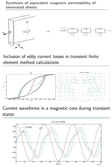
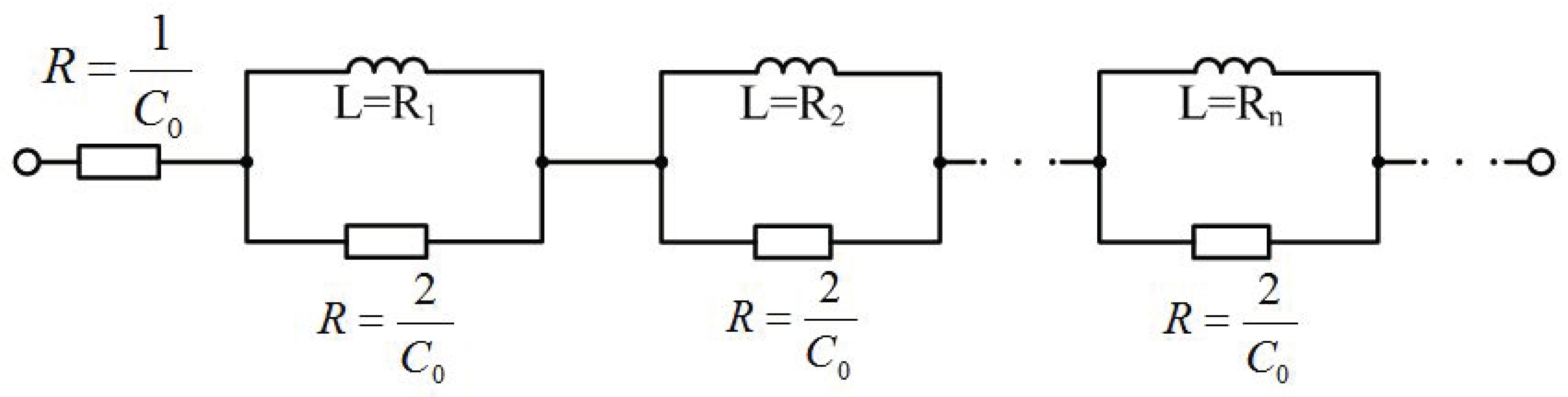
2.1. Direct Synthesis of Equivalent Magnetic Permeability of Laminated Sheets in the Form of a Transfer Function of an IIR Filter

In the presented method, the complex permeability, $\widehat{\mu }$, of a laminated magnetic core is derived. It can be expressed by impedance of the R, C system presented in Figure 1. In a similar manner, the complex reluctivity of a laminated core, $\widehat{\nu }=\frac{1}{\widehat{\mu }}$, may be expressed through impedance of the R, L circuit presented in Figure 2. The imaginary part of the magnetic permeability corresponds to active power, the real part to reactive power. These circuits should be treated as IIR filters, the transmittance of which comprises the representation of the equivalent magnetic permeability of a laminated core in the domain of the complex variable s of the Laplace transform. The equivalent magnetic permeability can be derived from Figure 3 and Formula (8) [29,30]. In order to include the saturation of the magnetic circuit in these calculations, an iterative process was developed. A scalar magnetic hysteresis model according to Juhani Tellinen has been implemented to also include hysteresis losses [31].

In order to consider the magnetic field in the transformer metal sheet, it is necessary to solve Maxwell’s equations in the coordinate system, as shown in Figure 3 [4,32]. We assume that the height of the plate in the x direction and its length along the y axis are infinitely large, and the magnetic flux density has only the y component. The magnetic field evokes a current that has a component in the x-axis direction and that is unevenly distributed in the z-axis direction with the density of $I\left(z\right)$. Maxwell’s equations are used then.

$$rot\overrightarrow{H}=\overrightarrow{J}=\gamma \overrightarrow{E}$$

(7)

$$rot\overrightarrow{E}=\frac{-\partial \overrightarrow{B}}{\partial t}=-j\omega \mu \overrightarrow{H}\Rightarrow rot(rot(\overrightarrow{H}))=-j\omega \mu \gamma \overrightarrow{H}\Rightarrow \frac{d^2{H}_y}{d{z}^2}=j\omega \mu \gamma H_y$$

(8)

where $\mu$ is the magnetic permeability of iron plate and $\gamma$ is the electric conductivity.

According to the considerations in [29], the formula was obtained for the mean value of the magnetic flux density in the plate $B_{avr}$ and for the complex magnetic permeability $\widehat{\mu }$:

$$B_{avr}=[\frac{2\mu }{p·d}·tanh(p\frac{d}{2})]·I$$

(9)

$$\widehat{\mu }=\frac{2\mu }{p·d}·tanh(p\frac{d}{2})$$

(10)

where $p=\sqrt{j·\omega ·\mu ·\gamma }$, while $\gamma$ is the material conductivity and $\mu$ is the magnetic permeability.

The Equations (9) and (10) are valid for mono-harmonic waveforms of the given angular frequency $\omega$. In order to obtain equations for any transient waveforms in time, it is necessary to substitute $j·\omega$ with the Laplace variable s. This substitution enables a shift from ‘details’, i.e., mono-harmonic waveforms, to ‘generality’, i.e., transient waveforms. Therefore, it is not always easy to perform it. However, it is used, for example, in the theory of digital filters, in order to derive equations for the transmittance of Butterworth or Czybyszew filters. Then, it is necessary to assume $p=\sqrt{s·\mu ·\gamma }$. The magnetic permeability in Equation (10) assumes an operational form, in which there occurs $\sqrt{s}$. In order to transform this permeability to the form of a rational function of Laplace’s variable s, it is possible to make use of the methods connected with fractional derivatives. When deriving Equation (11), an inverse Laplace transform [29] was used.

According to [29], the equivalent magnetic permeability of sheets from the Formula (10) can be represented in the form of the relationship:

$$\widehat{\mu }=\frac{1}{s[\frac{1}{C_{0}s}+{\displaystyle \sum _{n=1}^{\infty }}\frac{R_n\frac{2}{C_{0}s}}{R_n+\frac{2}{C_{0}s}}]}=\frac{1}{\frac{1}{C_0}+{\displaystyle \sum _{n=1}^{\infty }}\frac{1}{\frac{C_0}{2}+\frac{1}{R_{n}s}}}$$

(11)

where $C_0=\frac{k_2}{k_1^2}=\mu$; $R_n=\frac{2k_2}{n^2·{\pi }^2}=\frac{1}{n^2}\frac{d^2\gamma }{2{\pi }^2}$; $n=1,2,\dots \infty$.

The equivalent magnetic permeability can then be replaced with the impedance of the circuit in Figure 1. For the purpose of practical calculations, the infinite number of R,C series circuits connected in parallel is reduced to the number of n. The remaining part, beginning with $n+1$, is replaced with one equivalent RC branch. The parameters of this branch are selected with optimization methods that provide the best approximation in the given angular frequency range. The calculations are done with complex numbers. The unknown elements are the investigated parameters R and C of the parallel equivalent branch. What is searched here is the minimum of the sum of absolute values from the differences in the magnetic permeability from Equation (10) and impedance of the system from Figure 1, limited to n of parallel branches for the selected angular frequencies from the selected range from several Hz to 5000 Hz. In such a case, the classical optimisation algorithms for a convex problems are sufficient. When considering a wider range of angular velocities, it seems that it would be reasonable to apply the newest algorithms presented in [33,34]. The articles show the problem of identification of guaranteed passive rational models for linear distribution structures. The identification is pursued in two separate steps: In the first step, the Vector Fitting algorithm is used for identification of the poles, then the identification of residues is formulated as a convex programming problem with constraints on the single terms of the pole-residue expansion.

The equivalent magnetic reluctance $\widehat{\nu }=\frac{1}{\widehat{\mu }}$ is in the denominator of Formula (11). It can be presented in the form of a formula:

$$\widehat{\nu }=\frac{1}{C_0}+\sum _{n=1}^{\infty }\frac{(R_n·s)·\frac{2}{C_0}}{(R_n·s)+\frac{2}{C_0}}$$

(12)

and in the form of the R,L impedance from Figure 2

Sample non-linear iron magnetization characteristics were used for calculations in the formula:

$$H=a_{1}B+a_3{B}^3+a_9{B}^9$$

(13)

where $a_1=398$; $a_3=30$; $a_9=55$.

The condition of using a given formula as a magnetic characteristic is the one-uniqueness. In Figure 4 the difference between the curves marked as 1 and 2 for the assumed value of the magnetic flux density B determines the hysteresis losses. It presents the implementation of Tellinen’s hysteresis model in the time calculations [29,35].

Figure 5 and Figure 6 show the coefficients of the polynomials in the numerator and the denominator of the IIR analogue filter representing the equivalent magnetic permeability $\widehat{\mu }\left(s\right)$ in Figure 1 in the function of the squared magnetic flux density $B^2$.

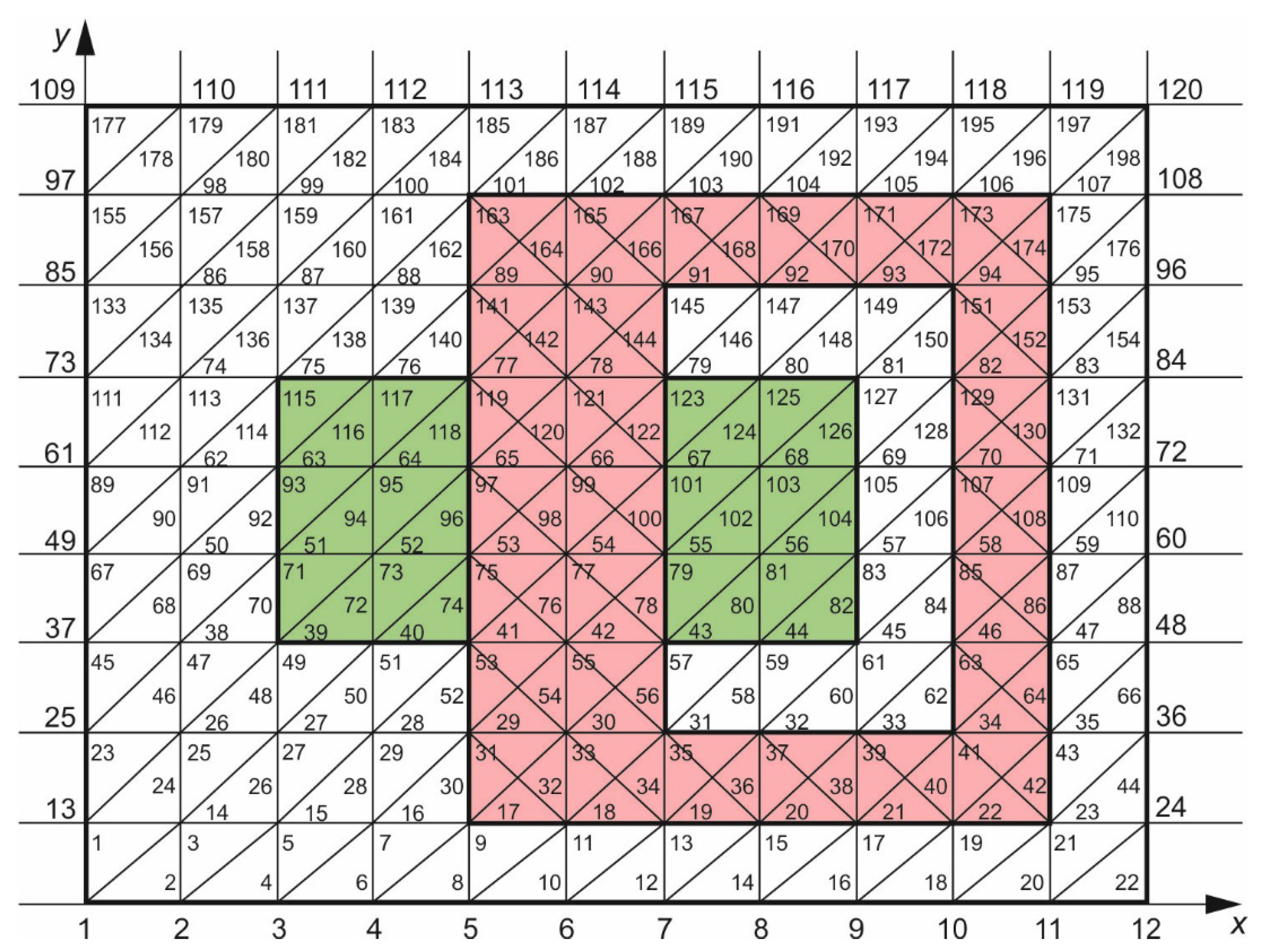
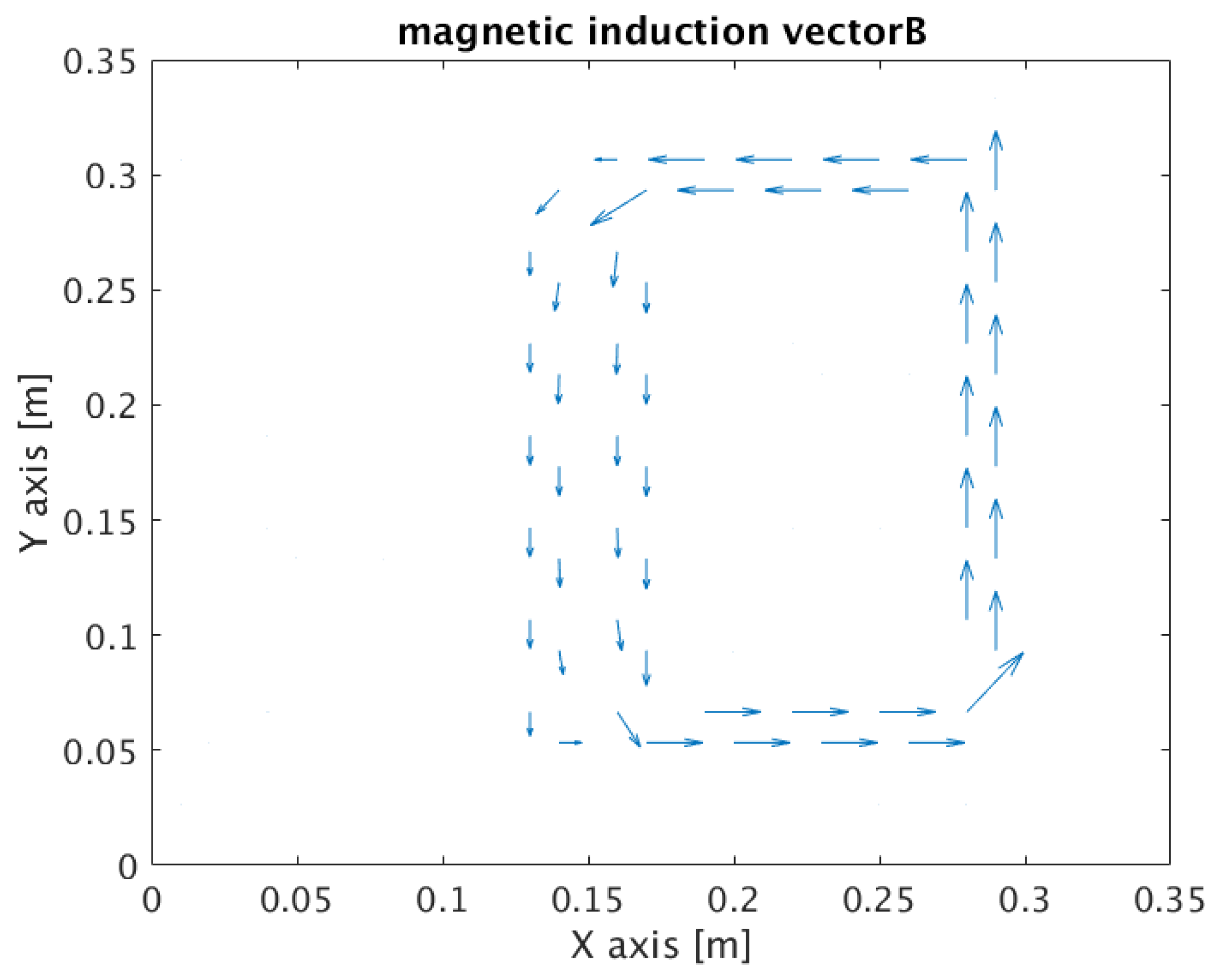
2.2. Inclusion of Eddy Current Losses in the Laminated Magnetic Circuit in Transient Finite Element Method Calculations

The transient state of the electric waveforms taking place in the choke should be calculated. A winding is wound on the magnetic core, which is switched on to a sinusoidal voltage. The magnetic core is made of laminated sheets, in which heat is released due to the eddy current losses. The system cross-section through the plane (x–y) is considered; therefore the symmetry along the coordinate axis z is assumed (Figure 7).

It is therefore necessary to calculate the magnetic flux density, $B(x,y)$, and the magnetic field strength, $H(x,y)$. A detailed derivation of the equation that describes the analyzed problem is presented in [36].

The equation that needs to be solved by means of the Finite Element Method assumes the following form:

$$\frac{\partial }{\partial x}(\frac{1}{{\mu }_x}\frac{\partial }{\partial x}{A}_z)+\frac{\partial }{\partial y}(\frac{1}{{\mu }_y}\frac{\partial }{\partial y}{A}_z)=-J_z$$

(14)

where ${\mu }_x$ and ${\mu }_y$ are the magnetic permeabilities.

It should be emphasized that, in this case, one is dealing with a magnetic anisotropic environment, thus ${\mu }_x\ne {\mu }_y$. According to the evidence presented in [37], it is necessary to apply rectangular coordinates $(x,y)$ connected with the environment. This manifests in the magnetic permeability ${\mu }_x$ along the x coordinate system and the magnetic permeability ${\mu }_y$ along the coordinate system of y. The current density $J_z$ should be dependent on the current flowing through the windings, which is a state variable. The magnetic permeability should include the eddy current losses in the laminated magnetic circuit, as described above. The cross-section x–y of the coil wound on the magnetic core is assumed, as shown in Figure 7 [31].

The coil is surrounded by air, and the whole system is contained in a rectangular area. We assume that the magnetic field does not escape outside the rectangle, therefore the zero Dirichlet Boundary Condition is imposed on the vector potential $A_z$ [38]. To apply the weak Galerkin formulation method, Equation (14) is multiplied by any variation of the vector potential $\sigma A$, using the following formula:

$$\sigma A·div(\frac{1}{\mu }·grad(\overrightarrow{A}))=div(\sigma A·\frac{1}{\mu }·grad(\overrightarrow{A}))-grad(\sigma A·\frac{1}{\mu }·grad(\overrightarrow{A}))$$

(15)

and then integrates over the entire section area [19,39]. When integrating the right side of the Formula (15), the Gauss theorem is used:

$${\int }_{V}div(\overrightarrow{R})·dV={\int }_S\overrightarrow{R}·\overrightarrow{dS}$$

(16)

where V is any volume limited by the surface S and vector $\overrightarrow{dS}$ is the vector of normal to elementary surface $dS$, directed outside the area V.

Zero Dirichlet conditions for the vector potential $\overrightarrow{A}$ were assumed at the boundary S. Therefore, the change of this potential, i.e., the variation at this boundary S, is also equal to zero. The first part of the right side of the Equation (15) is therefore zero, and the weak Galerkin formulation for Equation (14) can be noted as:

$${\int }_{V}grad(\sigma \overrightarrow{A})·\frac{1}{\mu \left(s\right)}·grad(\overrightarrow{A})dV-{\int }_V\sigma \overrightarrow{A}·J_{z}dV=0$$

(17)

where V is the x–y cross-section of the choke shown in Figure 7.

Formula (14) was used here. The left side of this formula, with the assumed symmetry to the axis z, is equal to: $div(\frac{1}{\mu }·grad(\overrightarrow{A}))=J_z$.

The system of equations of the finite element method is created by adding up the contributions from each finite element. Local coordinates are used [5]. The equivalent of the contribution of the first part of Formula (17) [5,31] to the general equation of the finite element method derived from the triangular finite element with linear shape functions is given by:

$$[\sigma A_i,\sigma A_j,\sigma A_m]\left\{\right[\begin{array}{c}{b}_i\\ b_j\\ b_m\end{array}]·\frac{1}{{\mu }_x\left(s\right)}·[\begin{array}{ccc}{b}_i& b_j& b_m\end{array}]+[\begin{array}{c}{c}_i\\ c_j\\ c_m\end{array}]+·\frac{1}{{\mu }_y\left(s\right)}·[\begin{array}{ccc}{c}_i& c_j& c_m\end{array}\left]\right\}·A·\left[\begin{array}{c}{A}_i\\ A_j\\ A_m\end{array}\right]$$

(18)

where $A_i$, $A_j$, $A_m$ are the searched magnetic potential values in triangle nodes and coefficients. The coefficients $b_i$, $b_j$, $b_m$ and $c_i$, $c_j$, $c_m$ depend on the difference between the global coordinate nodes of the Finite Element Method [5].

To determine the equivalent magnetic reluctance of the laminated core sheets, $\widehat{\nu }=\frac{1}{\mu }$, the Formula (12) is used. The magnetic reluctance $\widehat{\nu }\left(s\right)$ is obtained in the form of a rational function of the Laplace variable s, i.e., in the form of a transfer function of the IIR analogue filter. The system of equations obtained using the Finite Element Method is then multiplied by the IIR filter denominator to find the solution. Thanks to this multiplication, the $\widehat{\nu }\left(s\right)$ filter of the variable s will apply globally to all finite elements. This operation causes most of the computational costs and numerical difficulties in the presented procedure.

Formula (18) contains the essence of the implementation of the IIR filter, representing the equivalent magnetic permeability of laminated sheets, $\mu \left(s\right)$, for the Finite Element Model. The second segment of Equation (17), containing the current density $J_z$ should also be included in these calculations. This is the current density evenly distributed in the coil cross-section, caused by the coil current $I_c$. Therefore, the unknowns are: vector potential $\overline{u}=A_z$ and current $I_c$. The additional voltage equation should be created for the coil circuit, which is given by the Equation (19)

$${\int }_S{A}_z·{\rho }_{w}ds+L_{rs}·I_c+R_s·{\int }_0^t{I}_{c}dt={\int }_0^{t}Edt$$

(19)

where ${\rho }_w$ is the winding density in the cross-section S, $L_{rs}$ and $R_s$ are the leakage inductance and winding resistance, and $E\left(t\right)$ is the winding supply voltage.

In the case of a larger number of windings, a correspondingly larger number of additional equations must be taken into account. The alternative approach presented at this point, using the Laplace variable s to represent the equivalent magnetic permeability of transformer sheets of the magnetic circuit, will consist in multiplying each of the Equation (18) by denominators of rational functions $\widehat{\nu }\left(s\right)$ in the Laplace variable domain. The procedure during the implementation of the $\widehat{\nu }\left(s\right)$ filter for the Finite Element Method can, therefore, be called global. If different saturation levels of the magnetic circuit are included for different finite elements, then the presented procedure requires multiplication of the equations by the product of the IIR filter denominators, which can lead to further numerical difficulties.

The presented procedure causes that individual unknowns are to be multiplied by the appropriate degrees of the Laplace variable s, up to the coefficient $s^{N_{filter}-1}$, where $N_{filter}$ is the degree of the filter. The unknown creates a vector (the vector potential $A_z$ is marked by $\overline{u}$) $\overline{\left[XX\right]}=[\overline{u};\overline{I_c}]$. In order to avoid differentiations associated with the Laplace variable s, which may introduce large errors, the entire equation is additionally divided by $s^{N_{filter}-1}$ [2,32]. This corresponds to the division of the unknowns $\left[XX\right]$ by different degrees of the variable s. This means that the integrals will now be unknown: From the vector potential $\int udt=\int Adt$ and the integral from the current, $\int I_{c}dt$, as well as integrals of the higher degrees of these unknowns.

$$\left[XX\right]=\left[\begin{array}{c}\left[\begin{array}{c}\underset{0}{\overset{t}{\int }}udt\\ \underset{0}{\overset{t}{\int }}{I}_{c}dt\end{array}\right]\\ \left[\begin{array}{c}\underset{0}{\overset{t}{\int \int }}udtdt\\ \underset{0}{\overset{t}{\int \int }}{I}_{c}dtdt\end{array}\right]\\ \left[\begin{array}{c}\underset{0}{\overset{t}{\int \int \int }}udtdtdt\\ \underset{0}{\overset{t}{\int \int \int }}{I}_{c}dtdtdt\end{array}\right]\\ ⋮\end{array}\right];[pXX]=\frac{d}{dt}[XX]=\left[\begin{array}{c}\left[\begin{array}{c}u\\ I_c\end{array}\right]\\ \left[\begin{array}{c}\underset{0}{\overset{t}{\int }}udtdt\\ \underset{0}{\overset{t}{\int }}{I}_{c}dtdt\end{array}\right]\\ \left[\begin{array}{c}\underset{0}{\overset{t}{\int \int }}udtdtdt\\ \underset{0}{\overset{t}{\int \int }}{I}_{c}dtdtdt\end{array}\right]\\ ⋮\end{array}\right]$$

(20)

where the number of sub matrices with $n_1$ rows is equal to the highest degree of the variable s in the IIR filter transmittance, i.e., $N_{filter}-1$.

3. Results

Figure 8 presents the distribution of the magnetic flux density $\overrightarrow{B}$ in the tested cross-sectional area of the choke from Figure 7. The magnetic flux density closes mainly in the magnetic core of the choke. The course of the magnetic field strength vector $\overrightarrow{H}$, corresponding to the magnetic flux density in Figure 8, is shown in Figure 9.

Figure 10 shows the waveforms of the current $I_c$ and choke supply voltage $Ew$. Figure 11 shows the energies of the supply, sheet metal losses, and resistance losses. The correct balance of these energies indicates the correctness of the calculations. The energies accumulated in the leakage inductances in the air and in the winding area were small enough to be negligible here. In order to calculate the transient waveforms of the $Ic$ current and magnetic flux density $\overrightarrow{B}$, the losses in the laminated sheets are presented with the use of equivalent filters in the Laplace variable s domain.

When multiplying the system of equations of the finite element method by the IIR filter denominator representing the magnetic reluctance of sheets in the domain of variable s, the system of equations became global [39] and required extension of the state variables by their integrals (20) during integration with the Runge–Kutta method [40]. On the other hand, after performing the main FEM calculations for the post-process calculation of the magnetic field strength $\overrightarrow{H}$ in the finite elements, the IIR filter was used in the domain of the variable from the transformation Z. Calculations of this magnitude were, therefore, made locally for each finite element separately. The balancing of these quantities, as illustrated by the zero energy balance, is the evidence of the used method correctness. Similarly to energies, the momentary powers presented in Figure 12 were also balanced.

Similar waveforms, but for the angular frequency of $\omega =314.16$, are presented in Figure 13, Figure 14 and Figure 15.

The instantaneous power waveforms presented in Figure 12 and Figure 14 (angular frequency ${\omega }_1=3141.6$ and ${\omega }_2=314.16$ ) are presented in Figure 15 for the angular frequency ${\omega }_3=7854$.

4. Conclusions

The issue of appropriate modeling of the phenomena connected with the generation of losses in laminated magnetic cores of electric machines is significant from the perspective of the simulation result correctness of their transient states. Converter systems are being used increasingly more often to supply these machines. Non-sinusoidal character of the supply voltage waveforms additionally increase the power of losses, making the consideration of their influence on waveforms of machine dynamic states even more important, and making the modeling more difficult. A majority of methods for modelling losses in laminated cores that are known in the reference works, are of estimative character and require a previous determination of the waveforms of the machine dynamic states. Due to this fact, they do not provide the possibility to correctly consider the influence of the presence of losses in the core on the machine dynamic properties.

Few methods that have been proposed up to now provide the possibility to consider losses in laminated cores directly during the calculations of machine dynamics and they are characterized by very high computational complexity, which significantly limits their application in practice. This elaboration presents a model of equivalent magnetic permeability of a laminated magnetic core, in the form of an IIR filter. The model was then incorporated in the procedure of fast computations of electric machine dynamic waveforms, by means of the Finite Element Method. With the example of a choke, a series of simulation tests were performed. Correctness verification of the obtained results was done by means of a detailed balance of energy and power in the investigated system.

In compliance with the expectations, the results indicate a strong influence of the skin phenomenon on the value power of losses in the core. This effect is noticeable, in particular, by significant values of the magnetization frequency and a high magnetic permeability of the core. Additionally, these observations prove that the developed model allows for correct reflection of the phenomena that take place in the laminated magnetic core in the calculations of machine dynamics. The acquired values of the power of losses are adequate to the ones included in norms DIN EN 10106 and DIN EN 10207, which describe the magnetic properties of transformer sheets and the results of measurement experiments concerning determination of the power of losses in laminated cores.

A drawback of the presented method is the problematic necessity of global influence of the IIR filter on the system of equations of the Finite Element Method. In the follow-up studies, a solution of this problem is anticipated, by means of developing a model of equivalent magnetic permeability of a laminated core, in the form of a digital filter, possibly to implement in every finite element of the FE model separately. The aim of these efforts is to increase the efficiency of the numerical simulation procedure, so that it might find practical application in analyses of the dynamics of electric machine models.

References

1. Senda, K.; Uesaka, M.; Yoshizaki, S.; Oda, Y. Electric Steel and Their Evaluation for Automobile Motors. World Electr. Veh. J. 2019, 10, 31. [Google Scholar] [CrossRef] [Green Version]
2. Gołębiowski, L.; Lewicki, J. Electromagnetic Systems in Power Electronics; Printing House of Rzeszow University of Technology: Rzeszów, Poland, 2012. (In Polish) [Google Scholar]
3. Chen, W.; Ma, J.; Huang, X.; Fang, Y. Predicting Iron Losses in Laaminated Steel with Given Non-Sinusoidal Waveforms of Flux Density. Energies 2015, 8, 13726–13740. [Google Scholar] [CrossRef] [Green Version]
4. Demenko, A. Discrete methods of magnetic field description. Electrotech. Rev. 2009, 85, 107–110. (In Polish) [Google Scholar]
5. Jin, J. The Finite Element Method in Electromagnetics, 3rd ed.; Wiley-IEEE Press: Hoboken, NJ, USA, 2014. [Google Scholar]
6. Belahcen, A.; Arkkio, A. Comprehensive Dynamic Loss Model of Electrical Steel Applied to FE Simulation of Electrical Machines. IEEE Trans. Magn. 2008, 44, 886–889. [Google Scholar] [CrossRef]
7. Bermúdez, A.; Gómez, D.; Salgado, P. Eddy-Current Losses in Laminated Cores and the Computation of an Equivalent Conductivity. IEEE Trans. Magn. 2008, 44, 4730–4738. [Google Scholar] [CrossRef]
8. Bertotti, G. General properties of power losses in soft ferromagnetic materials. IEEE Trans. Magn. 1988, 24, 621–630. [Google Scholar] [CrossRef]
9. Bertotti, G. Hysteresis in Magnetism; IEEE Academic Press: San Diego, CA, USA, 1998. [Google Scholar]
10. Boglietti, A.; Cavagnino, A. Iron Loss Prediction with PWM Supply: An Overview of Proposed Methods from an Engineering Application Point of View. In Proceedings of the 2007 IEEE Industry Applications Annual Meeting, New Orleans, LA, USA, 23–27 September 2007; pp. 81–88. [Google Scholar]
11. Boglietti, A.; Cavagnino, A.; Lazzari, M.; Pastorelli, M. Predicting iron losses in soft magnetic materials with arbitrary voltage supply: An engineering approach. IEEE Trans. Magn. 2003, 39, 981–989. [Google Scholar] [CrossRef]
12. Boglietti, A.; Cavagnino, A.; Lazzari, M.; Pastorelli, M. Two simplified methods for the iron losses prediction in soft magnetic materials supplied by PWM inwerter. In Proceedings of the IEEE International Electric Machines and Drives Conference (Cat. No. 01EX485), Boston, MA, USA, 17–20 June 2001; pp. 391–395. [Google Scholar]
13. Ionel, D.; Popescu, M.; Dellinger, S.J.; Miller, T.J.E.; Heideman, R.J.; McGilp, M.I. Computation of core losses in electrical machines using improved model for laminated steel. IEEE Trans. Ind. Appl. 2007, 43, 1554–1564. [Google Scholar] [CrossRef] [Green Version]
14. Wang, J.; Lin, H.; Huang, Y.; Sun, X. A New Formulation of Anisotropic Equivalent Conductivity in Laminations. IEEE Trans. Magn. 2010, 47, 1378–1381. [Google Scholar] [CrossRef]
15. Zhu, S.; Cheng, M.; Dong, J.; Du, J. Core loss analysis and calculation of stator permanent-magnet machine considering dc-biased magnetic induction. IEEE Trans. Ind. Electron. 2014, 61, 5203–5212. [Google Scholar] [CrossRef]
16. Novak, G.; Kokošar, J.; Nagode, A.; Petrovi, D.S. Core-Loss Prediction for Non-Oriented Electrical Steels Based on the Steinmetz Equation Using Fixed Coefficients with a Wide Frequency Range of Validity. IEEE Trans. Magn. 2014. [Google Scholar] [CrossRef]
17. Tietz, M.; Biele, P.; Jansen, A.; Herget, F.; Telger, K.; Hameyer, K. Application-specific development of non oriented electrical steel for EV traction drives. In Proceedings of the 2nd International Electric Drives Production Conference (EDPC), Nuremberg, Germany, 15–18 October 2012; pp. 1–5. [Google Scholar]
18. Barbisio, E.; Fiorillo, F.; Ragusa, C. Predicting loss in magnetic steels under arbitrary induction waveform and with minor hysteresis loops. IEEE Trans. Magn. 2004, 40, 1810–1819. [Google Scholar] [CrossRef] [Green Version]
19. Mthombeni, L.T.; Pillay, P. Core losses in motor laminations exposed to high frequency or nonsinusoidal excitation, Industry Applications. IEEE Trans. Magn. 2004, 40, 1325–1332. [Google Scholar]
20. Exnowski, S. Transientes Verhalten des Wickelkopfes groser Turbogeneratoren bei unterschiedlichen Betriebszuständen. Ph.D. Thesis, Der Fakultät für Elektrotechnik und Informationstechnik der Technischen Universität Dortmund vorgelegte, Dortmund, Germany, 2009. [Google Scholar]
21. Łukaniszyn, M.; Jagieła, M.; Wróbel, R. Electromechanical Properties of a Disc-type Salient-pole Brushless DC Motor with Different Pole Numbers. COMPEL 2003, 22, 285–303. [Google Scholar] [CrossRef]
22. Łukaniszyn, M.; Jagieła, M.; Wróbel, R. Field-circuit analysis of construction modifications of a torus-type PMDC motor. COMPEL 2003, 22, 337–355. [Google Scholar] [CrossRef]
23. Shintemirov, A.; Tang, W.H.; Wu, Q.H. Transformer Core Parameter Identification Using Frequency Response Analysis. IEEE Trans. Magn. 2010, 46, 141–149. [Google Scholar] [CrossRef]
24. Lin, D.; Zhou, P.; Fu, W.N.; Badics, Z.; Cendes, Z.J. A dynamic core loss model for soft ferromagnetic and power ferrite materials in transient finite element analysis. IEEE Trans. Magn. 2004, 40, 1318–1321. [Google Scholar] [CrossRef]
25. Gyselinck, J.; Sabariego, R.V.; Dular, P. A Nonlinear Time-Domain Homogenization Technique for Laminated Iron Cores in Three-Dimensional Finite-Element Models. IEEE Trans. Magn. 2006, 42, 763. [Google Scholar] [CrossRef]
26. Rasilo, P.; Arkkio, A. Modeling the Effect of Inverter Supply on Eddy-Current Losses in Synchronous Machines. In Proceedings of the SPEEDAM 2010, Pisa, Italy, 14–16 June 2010. [Google Scholar]
27. Gyselinck, J.; Robert, F. Frequency- and Time-Domain Homogenization of Windings in Two-Dimensional Finite-Element Models. Gdzieś Nie Wiadomo Gdzie 2014, 61, 5203–5212. [Google Scholar]
28. Shindo, Y.; Miyazaki, T.; Matsuo, T. Cauer Circuit Representation of the Homogenized Eddy-Current Field Based on the Legendre Expansion for a Magnetic Sheet. IEEE Trans. Magn. 2016, 52, 6300504. [Google Scholar] [CrossRef]
29. Gołębiowski, M. Calculation of eddy current and hysteresis losses during transient states in laminated magnetic circuits. Compel 2017, 36, 665–682. [Google Scholar] [CrossRef]
30. Gołębiowski, L.; Mazur, D. Comparison of calculations methods of dissipation inductance in DC- supplied multiple-winding autotransformers. In Proceedings of the 21st Symposium of Electromagnetic Phenomena in Nonlinear Circuits (EPNC), Dortmund and Essen, Germany, 29 June–2 July 2010; pp. 55–56. [Google Scholar]
31. Gołębiowski, L.; Kulig, S.T. Numerical Methods in Technology; Printing House of Rzeszow University of Technology: Rzeszów, Poland, 2012. (In Polish) [Google Scholar]
32. Bolkowski, S.; Stabrowski, M.; Skoczylas, J.; Sikora, J.; Wincenciak, S. Computer Aided Methods of Magnetic Field Analysis; WNT: Warszawa, Poland, 1993. (In Polish) [Google Scholar]
33. De Tommasi, L.; De Magistris, M.; Deschrijver, D.; Dhaene, T. An algorithm for direct identification of passive transfer matrices with positive real fractions via convex programming. Int. J. Numer. Model. Electron. Netw. Devices Fields 2011, 24, 375–386. [Google Scholar] [CrossRef] [Green Version]
34. De Tommasi, L.; de Magistris, M.; Deschrijver, D.; Dhaene, T. Validation of Positive Fraction Vector Fitting Algorithm in the identification of Passive Immittances. In Proceedings of the X-th International Workshop on Optimization and Inverse Problems in Electromagnetism, Ilmenau, Germany, 14–17 September 2008. [Google Scholar]
35. Tellinen, J. A Simple Scalar Model for Magnetic Hysteresis. IEEE Trans. Magn. 1998, 34, 2200–2206. [Google Scholar] [CrossRef]
36. Smoleń, A.; Gołębiowski, M. Computationally efficient method for determining the most important electrical parameters of Axial Field Permanent Magnet machine. Biuletin Yhe Pol. Acad. Sci. Tech. Sect. 2018, 66, 947–959. [Google Scholar]
37. Mayergoyz, I.D.; Abdel-Kader, F.M.; Emad, F.P. On penetration of electromagnetic fields into nonlinear conducting ferromagnetic media. J. Appl. Phys. 1984, 618. [Google Scholar] [CrossRef]
38. Coulomb, J.L. A methodology for the determination of global electromechanical quantities from a finite element analysis and its application to the evaluation of magnetic forces, torques and stiffness. IEEE Trans. Magn. 1983, 19, 2514–2519. [Google Scholar] [CrossRef]
39. Saad, Y. Numerical Methods for Large Eigenvalues Problems, 2nd ed.; Society for Industrial and Applied Mathematics: Philadelphia, PA, USA, 2011. [Google Scholar]
40. Nowak, L. Field Models Transients in Electromechanical Converters; Poznań University of Technology Publishing House: Wrocław, Poland, 1999. (In Polish) [Google Scholar]
Figure 1. Synthesis of the equivalent magnetic permeability, μ ^ , in the form of an R,C system.
Energies 13 01174 g001
Figure 2. The synthesis of the equivalent magnetic reluctivity ν ^ = 1 μ ^ in the form of an R,L system.
Energies 13 01174 g002
Figure 3. A magnetic field in the transformer plate induced by an external current with density I.
Energies 13 01174 g003
Figure 4. The dependence of the magnetic magnetic flux density B on the strength of the magnetic field H at frequency f = 1500 Hz; 1—the curve including losses of eddy current and hysteresis, 2—the curve including only eddy current losses, 3—the primary magnetization curve (10).
Energies 13 01174 g004
Figure 5. The diagram presents general dependency of the changeability of polynomial coefficients that comprise the numerator of the developed IIR filter in the domain of Laplace variable s, in the function of B 2 .
Energies 13 01174 g005
Figure 6. The diagram presents the general dependency of the changeability of polynomial coefficients that comprise the denominator of the developed IIR filter in the domain of the Laplace variable, s, in the function of B 2 .
Energies 13 01174 g006
Figure 7. The cross-section x–y of a coil wound on a magnetic core; red—cross-section of the magnetic core, green—cross-section through the coil.
Energies 13 01174 g007
Figure 8. The distribution of the magnetic flux density vector in the cross-sectional area of the choke for angular frequencies ω = 3141.6 rad s and time t = 0.1 s.
Energies 13 01174 g008
Figure 9. The distribution of the magnetic field intensity vector H corresponding to the magnetic flux density B from Figure 8 ω = 3141.6 rad s and time t = 0.1 s.
Energies 13 01174 g009
Figure 10. The waveform of the choke current I c ( * 100 ) and voltage supplying the choke E w for angular frequencies ω = 3141.6 rad s after switching it on.
Energies 13 01174 g010
Figure 11. The waveform of the power supply, energy loss in iron, energy loss of resistance, and a zero energy balance for angular frequencies ω = 3141.6 rad s .
Energies 13 01174 g011
Figure 12. The momentary power waveform in leakage inductance ( L s r ), power in the air area (air), power in the winding area (winding), which all increased 100 times, and the power loss in laminated sheets for angular frequencies ω = 3141.6 rad s .
Energies 13 01174 g012
Figure 13. The supply energy waveform, energy losses in iron, energy of losses of resistance, and zeroing energy balance for the angular frequencies ω = 3141.6 rad s .
Energies 13 01174 g013
Figure 14. The instantaneous power waveform in leakage inductance ( L r s ) of the power in the air space (air), power in the winding space (winding), all magnified 100 times, and the power of losses in laminated sheets for the angular frequencies ω = 3141.6 rad s .
Energies 13 01174 g014
Figure 15. The instantaneous power waveform in leakage inductance ( L r s ), in air space (pow), winding space power (uzw), all magnified 100 times, and the power of losses in laminated sheets for the angular frequencies ω = 3141.6 rad s .
Energies 13 01174 g015