Flow Allocation in Meshed AC-DC Electricity Grids

Abstract

In power systems, flow allocation (FA) methods enable to allocate the usage and costs of the transmission grid to each single market participant. Based on predefined assumptions, the power flow is split into isolated generator-specific or producer-specific sub-flows. Two prominent FA methods, Marginal Participation (MP) and Equivalent Bilateral Exchanges (EBEs), build upon the linearized power flow and thus on the Power Transfer Distribution Factors (PTDFs). Despite their intuitive and computationally efficient concepts, they are restricted to networks with passive transmission elements only. As soon as a significant number of controllable transmission elements, such as high-voltage direct current (HVDC) lines, operate in the system, they lose their applicability. This work reformulates the two methods in terms of Virtual Injection Patterns (VIPs), which allows one to efficiently introduce a shift parameter q to tune contributions of net sources and net sinks in the network. In this work, major properties and differences in the methods are pointed out, and it is shown how the MP and EBE algorithms can be applied to generic meshed AC-DC electricity grids: by introducing a pseudo-impedance $\overline{\mathit{\omega }}$, which reflects the operational state of controllable elements and allows one to extend the PTDF matrix under the assumption of knowing the current flow in the system. Basic properties from graph theory are used to solve for the pseudo-impedance in dependence of the position within the network. This directly enables, e.g., HVDC lines to be considered in the MP and EBE algorithms. The extended methods are applied to a low-carbon European network model (PyPSA-EUR) with a spatial resolution of 181 nodes and an 18% transmission expansion compared to today’s total transmission capacity volume. The allocations of MP and EBE show that countries with high wind potentials profit most from the transmission grid expansion. Based on the average usage of transmission system expansion, a method of distributing operational and capital expenditures is proposed. In addition, it is shown how injections from renewable resources strongly drive country-to-country allocations and thus cross-border electricity flows.

1. Introduction

The shift from conventional to renewable power sources requires high investments not only in terms of the generation but also in terms of the transmission and storage of a power system. Due to the dominant dependence on fluctuating wind and solar power potentials, energy has to be shifted in space and time. For large networks, such as the European power system, both elements will play a key role. Spatial balancing via a solid transmission grid allows power to cover long distances from wind farms to load centers far away. In contrast, temporal balancing allows for self-sufficient areas, which locally produce and store (most likely solar) power. This raises the question of the extent to which one uses and benefits from the transmission grid and its upcoming expansions. Flow allocation (FA) methods enable to efficiently quantify the transmission usage per market participant by decomposing the network flow into sub-flows driven by isolated power injections. This opens the opportunity to distribute transmission costs based on the effective transmission usage of each single generator and consumer, as broadly reviewed by Jiuping et al. [1]. It also helps in understanding the operational state of the system and in determining cost-increasing and cost-reducing actions and therefore in drawing up incentives or cost schemes for an efficient system transformation.

There are multiple flow allocation methods that all differently approach the determination of isolated sub-flows. The most prominent candidates are as follows:

(a)

Average Participation, also referred to as Flow Tracing, firstly presented by Bialek [2] and used in various application cases such as by Hoersch et al. [3]. It follows the principle of proportional sharing when tracing a power flow from source to sink.

(b)

Z-bus transmission allocation presented by Conejo et al. [4], which is equivalent to the Power Divider method [5] and strongly related to the formulation by Chang and Lu [6]. It derives the contributions of electricity current injections to the branch currents based on the full AC power flow equations.

(c)

Marginal Participation (MP) presented by Rudnick et al. [7] and the Equivalent Bilateral Exchange (EBE) method [8], which are based on the linearized power flow equations and extensively explained later in this paper.

(d)

With-And-Without transit loss allocation presented by Hadush et al. [9], which builds the underlying loss allocation for the Inter-Transmission System Operators Compensation (ITC) mechanism. In contrast to the other methods, it does not determine source-sink relations but calculates losses within regions or countries caused by cross-border flows.

Non-flow-based cost allocation includes another palette of methods, such as the Aumann-Shapley method [10], which is based on game theory or an exogenous approach [11], which proposes to introduce a peer-to-peer market design into the optimal power flow (OPF) calculation. Originally, FA methods focus on determining the flow shares on branches. However, the work by Schaefer et al. [12] shows that the FA can be alternatively represented through Virtual Injection Patterns (VIPs), which are peer-to-peer allocations between sources and sinks. Thus, every market generator is associated to a specific set of supplied loads; vice versa, loads are allocated to a specific set of power suppliers from which they retrieve their share. The artificial peer-to-peer transactions can then be used to, e.g., determine nodal electricity prices or the CO${}_2$-intensity of the consumed power, as done in a recent study by Tranberg et al. [13]. As all FA methods come with strengths and weaknesses, it turns out that most of them are restricted to pure AC or pure passive DC transmission networks only. This applies to non-linear FA as well as MP and EBEs, which rely on the linear Power Transfer Distribution Factors (PTDFs). It makes them inappropriate for large networks such as the European one, which consists of multiple AC subnetworks, i.e., synchronous zones operating at a specific utility frequency. PTDF-based allocation is not yet applicable over borders of these zones, and only conceptional propositions have been made to tackle this issue [14]. Note that FA on a distribution network level is also inappropriate for the MP and EBE algorithms, as the characteristics of high resistance-reactance ratios render the linear approximation of the power flow invalid. This restricts the scope of application of the MP and EBE algorithms considerably. However, this paper presents a way to apply the algorithms to meshed AC-DC transmission networks by incorporating controllable elements such as HVDC lines into the PTDF matrix.

This paper is structured as follows: Section 2 recalls the MP and EBE algorithms, focusing on both VIPs and flow share formulation. Section 3 describes the extension of the flow allocation methods for generic AC-DC networks, realized through the introduction of the so-called pseudo-reactance $\overline{\mathit{\omega }}$. In Section 4, the extended FA is performed for a highly renewable European power system, and Section 5 summarizes and concludes the paper.

2. PTDF-Based Flow Allocation Methods

The MP and EBE algorithms are both based on the linear power flow approximation. In order to recall and extend them, the following definitions are used in this work:

• Nodal active power $\mathbf{p}\in {\mathbb{R}}^N$
• Active power flow $\underline{\mathbf{f}}\in {\mathbb{R}}^L$
• Transmission reactance $\underline{\mathbf{x}}\in {\mathbb{R}}^L$
• Transmission resistance $\underline{\mathbf{r}}\in {\mathbb{R}}^L$
• Transmission admittance $\underline{\mathbf{y}}\in {\mathbb{C}}^L$
• Incidence matrix $\mathbf{K}\in {\mathbb{R}}^{N\times L}$
• PTDF matrix $\mathbf{H}\in {\mathbb{R}}^{L\times N}$
• Cycle matrix $\mathbf{C}\in {\mathbb{R}}^{L\times C}$
• Virtual Injection Pattern $\tilde{\mathbf{P}}\in {\mathbb{R}}^{N\times N}$
• Virtual Flow Pattern $\tilde{\mathbf{F}}\in {\mathbb{R}}^{L\times N}$
• Peer-to-Peer Allocations $\mathbf{A}\in {\mathbb{R}}^{N\times N}$

N denotes the number of buses in the system, L the number of branches (transmission lines), and C the number of cycles in the network. Note that the equality C = L − N + 1 holds as shown by Ronellenfitsch et al. [15,16]. The linear power flow approximation assumes that all bus voltage magnitudes are equal, ${\widehat{\mathrm{v}}}_i={\widehat{\mathrm{v}}}_j$, and the series resistances are small compared to series reactances, $r_l\ll x_l$. In addition, voltage angle differences across a line are assumed to be small, and no shunt admittances (at buses or series) to ground are present. These assumptions are usually appropriate for transmission systems, where high voltages and small resistances lead to a power flow that is mostly driven by active power injection $\mathbf{p}$. They allow one to map the latter linearly to the active power flow $\underline{\mathbf{f}}$ through the PTDF matrix

$$\begin{array}{cc}\hfill \underline{\mathbf{f}}& =\mathbf{H}\mathbf{p}\hfill \end{array}$$

(1)

where the PTDF matrix is defined as

$$\begin{array}{cc}\hfill \mathbf{H}& =diag\left(\underline{\mathbf{y}}\right){\mathbf{K}}^T{\left(\mathbf{K}diag\left(\underline{\mathbf{y}}\right){\mathbf{K}}^{\mathrm{T}}\right)}^{+}\hfill \end{array}$$

(2)

with the series admittance $\underline{\mathbf{y}}={\underline{\mathbf{x}}}^{-1}$ and with ${\left(\right)}^{+}$ denoting the generalized inverse. We recall that the PTDF matrix can be provided with a slack, which is one or more buses that “absorb” the total power imbalances of $\mathbf{p}$. In Equation (2), the slack is distributed over all nodes in the system, but it is possible to modify it by adding a column vector $\mathbf{k}$ to each column of the PTDF matrix

$$\begin{array}{c}\hfill \mathbf{H}\to \mathbf{H}+\mathbf{k}\end{array}$$

(3)

without touching the result of the linear power flow expressed by Equation (1) for a balanced injection pattern (note that the vector addition in (3) is applied to every column of $\mathbf{H}$). Corresponding to Equation (1), the nodal power balance is expressed by

$$\begin{array}{c}\hfill \mathbf{p}=\mathbf{K}\underline{\mathbf{f}}.\end{array}$$

(4)

As pointed out earlier, the FA methods can be perceived from two different angles. One is looking at the impact of generators or consumers on the network flow that they cause in the network, respectively. The Virtual Flow Pattern (VFP) matrix $\tilde{\mathbf{F}}$ is an L × N matrix, whose nth column denotes the sub-flows induced by bus n. The other is looking at the peer-to-peer transactions given by the VIP matrix $\tilde{\mathbf{P}}$ of size N × N, whose nth column denotes the effective balanced injection pattern of bus n. The two quantities contain the same information and are, like Equations (1) and (4), linked through

$$\begin{array}{c}\hfill \tilde{\mathbf{F}}=\mathbf{H}\tilde{\mathbf{P}}\end{array}$$

(5)

and

$$\begin{array}{c}\hfill \tilde{\mathbf{P}}=\mathbf{K}\tilde{\mathbf{F}}.\end{array}$$

(6)

The sum of their columns equals the original flow,

$$\begin{array}{c}\hfill \underline{\mathbf{f}}=\tilde{\mathbf{F}}{\mathbf{1}}_N\end{array}$$

(7)

and the original injection pattern,

$$\begin{array}{c}\hfill \mathbf{p}=\tilde{\mathbf{P}}{\mathbf{1}}_N\end{array}$$

(8)

where ${\mathbf{1}}_N$ represents a vector of ones of length N. Furthermore, let $\mathbf{A}$ denote an $N\times N$ matrix with peer-to-peer transactions $m\to n$ given by the entry $A_{mn}$. For a given VIP matrix, those values are straightforwardly obtained by ${\tilde{P}}_{mn}-{\tilde{P}}_{nm}$, which is taking all power in the injection pattern of n coming from m to n and all the negative power in the injection pattern of n coming from m. In matrix notation, this leads to

$$\begin{array}{c}\hfill \mathbf{A}={\left(\tilde{\mathbf{P}}-{\tilde{\mathbf{P}}}^{\mathrm{T}}\right)}_{+}\end{array}$$

(9)

where ${\left(\right)}_{+}$ denotes a restriction to positive entries only. The latter should be taken for granted as only positive source to sink relations are considered. Thus, for non-zero values $A_{mn}$, bus m is always a net producer and bus n a net consumer.

2.1. Equivalent Bilateral Exchanges

The definition of the EBE algorithm refers to peer-to-peer exchanges between net producers (sources) and net consumers (sinks) in the network [8]. It assumes that a source provides power to all sinks in the network, which are proportionally scaled down until positive and negative injections are balanced, while all other sources are ignored. Correspondingly, it assumes that power flowing into a sink comes from all sources, which are proportionally scaled down until positive and negative injections are balanced, while all other sinks are ignored. In order to allow weighting the net producers differently from net consumers, let $0\le q\le 1$ be a shift parameter that allows one to tune their contributions (the lower the value of this shift parameter is, the stronger the net consumers taken into account are). Furthermore, let ${\mathbf{p}}_{+/-}$ denote injections by only sources/sinks and let $\gamma ={\left({\mathbf{p}}_{+}^{\mathrm{T}}{\mathbf{1}}_N\right)}^{-1}$ denote the inverse of the total positive injected power. Therefore, the VIP is given by

$$\begin{array}{c}\hfill {\tilde{\mathbf{P}}}_{\mathrm{ebe}}=q\left({\mathbf{P}}_{+}+\gamma {\mathbf{p}}_{-}{\mathbf{p}}_{+}^{\mathrm{T}}\right)+(1-q)\left({\mathbf{P}}_{-}-\gamma {\mathbf{p}}_{+}{\mathbf{p}}_{-}^{\mathrm{T}}\right).\end{array}$$

(10)

The first term represents injection patterns of net producers only, which deliver power to sinks. The second term comprises injection patterns of all net consumers. The corresponding VFP matrix ${\tilde{\mathbf{F}}}_{\mathrm{ebe}}$ is given by

$$\begin{array}{cc}\hfill {\tilde{\mathbf{F}}}_{\mathrm{ebe}}\left(q\right)& =\mathbf{H}{\tilde{\mathbf{P}}}_{\mathrm{ebe}}\left(q\right).\hfill \end{array}$$

(11)

If q is set to 0.5, 50% of the flow is allocated to net producers, and 50% to net consumers. Inserting Equation (10) into Equation (11) allows one to write the VFP as

$$\begin{array}{c}\hfill {\tilde{\mathbf{F}}}_{\mathrm{ebe}}=\mathbf{H}\mathbf{P}\end{array}$$

(12)

with a given slack of $\mathbf{k}=\gamma {\underline{\mathbf{f}}}_{-}$ for net producers and of $\mathbf{k}=-\gamma {\underline{\mathbf{f}}}_{+}$ for net consumers in the PTDF matrix (see Equation (3)). It is taken as granted that the separate flow patterns induced by the market participants can be of a completely different nature than the original flow. Therefore, the FA method may lead to counter-flows that are counter-aligned to the network flow $\underline{\mathbf{f}}$.

Given that $\mathbf{p}={\mathbf{p}}_{+}+{\mathbf{p}}_{-}$, the peer-to-peer relations are straightforwardly obtained by first reformulating (10) to

$$\begin{array}{cc}\hfill {\tilde{\mathbf{P}}}_{\mathrm{ebe}}& ={\mathbf{P}}_{-}-\gamma {\mathbf{p}}_{+}{\mathbf{p}}_{-}^{\mathrm{T}}+\underset{\mathrm{symmetric}}{\underbrace{q\left(\left|\mathbf{P}\right|+\gamma {\mathbf{p}}_{-}{\mathbf{p}}_{+}^{\mathrm{T}}+\gamma {\mathbf{p}}_{+}{\mathbf{p}}_{-}^{\mathrm{T}}\right)}}\hfill \end{array}$$

(13)

and second inserting the new expression into Equation (9) ($|·|$ denotes the absolute value). Note that the symmetric term cancels out, which makes $\mathbf{A}$ independent of q, and finally reduces it to

$$\begin{array}{c}\hfill {\mathbf{A}}_{\mathrm{ebe}}=-\gamma {\mathbf{p}}_{+}{\mathbf{p}}_{-}^{\mathrm{T}},\end{array}$$

(14)

which, one on one, reflects the definition of the EBE flow allocation.

2.2. Marginal Participation

The MP algorithm, in contrast to EBEs, derives from a sensitivity-analyzing perspective that directly defines the VFP matrix. As originally proposed, it measures each line’s active power flow sensitivity against changes in the power balances of the buses. The sensitivity characteristics are then multiplied with the nodal power imbalances, which gives the sub-flows induced by the buses. As the work of Brown [14] describes in detail, the choice of the slack $\mathbf{k}$ is used to tune contributions of net producers and net consumers. However, aiming at introducing the shift parameter q correctly and in a generalized way, we propose straightforwardly to define the VIP matrix as

$$\begin{array}{cc}\hfill {\tilde{\mathbf{P}}}_{\mathrm{mp}}& ={\tilde{\mathbf{P}}}_{\mathrm{ebe}}+s\left(\mathbf{P}+\gamma {\mathbf{p}}_{-}{\mathbf{p}}_{-}^{\mathrm{T}}-\gamma {\mathbf{p}}_{+}{\mathbf{p}}_{+}^{\mathrm{T}}\right)\hfill \end{array}$$

(15)

where s is set to $s=\frac{1}{2}-\left|q-\frac{1}{2}\right|$. Here, we used the full VIP for the EBE method and added a term that only takes effect for $0<q<1$. This makes ${\tilde{\mathbf{P}}}_{\mathrm{mp}}$ and ${\tilde{\mathbf{P}}}_{\mathrm{ebe}}$ the same for full allocation to consumers ($q=0$) or producers ($q=1$). The standard 50–50% split leads to

$$\begin{array}{cc}\hfill {\tilde{\mathbf{P}}}_{\mathrm{mp}}(q=0.5)& =\mathbf{P}-{\displaystyle \frac{1}{2}}\gamma \left|\mathbf{p}\right|{\mathbf{p}}^{\mathrm{T}},\hfill \end{array}$$

(16)

which, when inserting into Equation (5), leads to an effective slack of

$$\begin{array}{c}\hfill {\mathbf{k}}_{\mathrm{mp}}(q=0.5)={\displaystyle \frac{1}{2}}\gamma \left({\underline{\mathbf{f}}}_{-}-{\underline{\mathbf{f}}}_{+}\right),\end{array}$$

(17)

which reflects the standard setup of the MP algorithm as originally proposed. Overall, the newly introduced formulation given in Equation (15) generalizes the algorithm for the shift parameter q and matches the EBE method for full consumer/producer contributions. Again note that the ${\tilde{\mathbf{F}}}_{\mathrm{MP}}$ may contain counter-flows that are not aligned with $\underline{\mathbf{f}}$. Especially in the realm around $q=0.5$, this is even more likely for the MP method, as flows are also allocated from one net producer to another net producer. It shall be noted that the second term in Equation (15) is symmetric, which makes the peer-to-peer allocation again independent of the shift parameter q and leads to

$$\begin{array}{c}\hfill {\mathbf{A}}_{\mathrm{mp}}=-\gamma {\mathbf{p}}_{+}{\mathbf{p}}_{-}={\mathbf{A}}_{\mathrm{ebe}}.\end{array}$$

(18)

It can the be concluded that the peer-to-peer relations for both EBE and MP are the same, whereas the flow allocations and virtual injections patterns differ for mixed producer-consumer contributions.

3. Including Controllable Elements in the PTDF Formulation

Despite representing the two methods in the form of VIPs, Equations (10) and (15), the flow allocation in the form of Equation (5) is still restricted to the scope of the PTDF matrix, namely to AC subnetworks or pure passive DC networks. Up to now, proposals for incorporating HVDC lines within the MP or EBE algorithms [14,17] are rather of a conceptional nature and do not derive all mathematical details. In the following, it is shown how the PTDF matrix can be reformulated and extended by introducing a flow-dependent pseudo-impedance $\overline{\mathit{\omega }}\left(\underline{\mathbf{f}}\right)$ for controllable DC lines, which here shall represent all controllable branch elements. The resulting extended PTDF matrix then solves Equation (1) for mixed AC-DC networks.

In a network of N nodes and L lines, let there be ${\mathrm{L}}_{\mathrm{AC}}$ AC lines, ${\mathrm{L}}_{\mathrm{PDC}}$ passive DC lines, and ${\mathrm{L}}_{\mathrm{CDC}}$ controllable DC lines. As stated by Ronellenfitsch et al. [15], a graph can always be decomposed into cycles and trees. Due to different physical laws, the two cases are treated separately, in terms of a DC line being part of a cycle in the network (Case 1) or being part of a tree in the network (Case 2).

3.1. Controllable Elements in Cycles (Case 1)

Let ${\mathbf{C}}^{\mathrm{AC}}$ denote the cycle matrix for all pure AC line cycles and ${\underline{\mathbf{f}}}^{\mathrm{AC}}\in {\mathbb{R}}^{{\mathrm{L}}_{\mathrm{AC}}}$ be the flow on all AC lines, then, according to the linear approximation, the Kirchhoff voltage law states that the flows in every closed cycle weighted by the reactants sum up to zero, namely

$$\begin{array}{cc}\hfill {\mathbf{C}}^{\mathrm{AC}}diag\left(\underline{\mathbf{x}}\right){\underline{\mathbf{f}}}^{\mathrm{AC}}& =0.\hfill \end{array}$$

(19)

As a counterpart, let ${\mathbf{C}}^{\mathrm{PDC}}$ be the cycle matrix for passive DC lines and ${\underline{\mathbf{f}}}_{\mathrm{passive}}^{\mathrm{DC}}$ the flow on those lines. Ohm’s law states that flows in a closed cycle weighted by underlying resistances sum up to zero:

$$\begin{array}{c}\hfill {\mathbf{C}}^{\mathrm{PDC}}diag\left(\underline{\mathbf{r}}\right){\underline{\mathbf{f}}}_{\mathrm{passive}}^{\mathrm{DC}}=0.\end{array}$$

(20)

In a network with pure AC subnetworks and pure passive DC subnetworks, $\underline{\mathbf{x}}$ and $\underline{\mathbf{r}}$ are not overlapping. Equations (19) and (20) can thus be combined by using $\underline{\mathbf{z}}={\left[\begin{array}{c}\underline{\mathbf{r}}\underline{\mathbf{x}}\end{array}\right]}^{\mathrm{T}},\underline{\mathbf{z}}\in {\mathbb{R}}^{L-L_{\mathrm{CDC}}}$ and collecting the flows on all passive branches in ${\underline{\mathbf{f}}}_{\mathrm{passive}}={\left[\begin{array}{c}{\underline{\mathbf{f}}}^{\mathrm{AC}}{\underline{\mathbf{f}}}_{\mathrm{passive}}^{\mathrm{DC}}\end{array}\right]}^{\mathrm{T}}$, which leads to

$$\begin{array}{cc}\hfill \left[\begin{array}{c}{\mathbf{C}}^{\mathrm{AC}}\\ {\mathbf{C}}^{\mathrm{PDC}}\end{array}\right]diag\left(\underline{\mathbf{z}}\right){\underline{\mathbf{f}}}_{\mathrm{passive}}& =0.\hfill \end{array}$$

(21)

Note that flows on controllable DC lines are not considered in Equation (21), as those are not given by physical laws and are not a function of $\left(\mathbf{C},\underline{\mathbf{r}},\mathbf{p}\right)$. In order to include controllable DC lines, let ${\mathbf{C}}^{\mathrm{mixed}}$ denote the cycle matrix with all cycles in which (I) controllable DC lines with nonzero flow appear and (II) no controllable DC line with zero flow are present. Note that (II) guarantees that topologically irrelevant cycles are excluded as controllable DC with zero flow are not affecting the total flow pattern. We introduce a pseudo-impedance $\overline{\mathit{\omega }}\in {\mathbb{R}}^{L_{\mathrm{CDC}}}$ for controllable DC lines, which fulfills the following equation:

$$\begin{array}{cc}\hfill \mathbf{C}diag\left(\left[\begin{array}{c}\underline{\mathbf{z}}\\ \overline{\mathit{\omega }}\end{array}\right]\right)\underline{\mathbf{f}}& =0\hfill \end{array}$$

(22)

where $\mathbf{C}$ denotes all cycles in the AC/DC super grid in the form $\mathbf{C}={\left[\begin{array}{c}{\mathbf{C}}^{\mathrm{AC}}{\mathbf{C}}^{\mathrm{PDC}}{\mathbf{C}}^{\mathrm{mixed}}\end{array}\right]}^{\mathrm{T}}$ and $\underline{\mathbf{f}}$ the full network flow in the form $\underline{\mathbf{f}}={\left[\begin{array}{c}{\underline{\mathbf{f}}}_{\mathrm{passive}}{\underline{\mathbf{f}}}_{\mathrm{control}.}\end{array}\right]}^{\mathrm{T}}$. In order to solve Equation (22) for $\overline{\mathit{\omega }}$, we only consider mixed cycles, since all other cycles are not affected by $\overline{\mathit{\omega }}$. We then split the mixed cycle matrix according to ${\mathbf{C}}^{\mathrm{mixed}}=\left[\begin{array}{c}{\mathbf{C}}_{\mathrm{passive}}^{\mathrm{mixed}}{\mathbf{C}}_{\mathrm{control}.}^{\mathrm{mixed}}\end{array}\right]$ into two parts:

$$\begin{array}{cc}\hfill 0& ={\mathbf{C}}^{\mathrm{mixed}}diag\left(\left[\begin{array}{c}\underline{\mathbf{z}}\\ \overline{\mathit{\omega }}\end{array}\right]\right)\underline{\mathbf{f}}\hfill \end{array}$$

(23)

$$\begin{array}{cc}\hfill & =\left[\begin{array}{c}{\mathbf{C}}_{\mathrm{passive}}^{\mathrm{mixed}}{\mathbf{C}}_{\mathrm{control}.}^{\mathrm{mixed}}\end{array}\right]diag\left(\left[\begin{array}{c}\underline{\mathbf{z}}\\ \overline{\mathit{\omega }}\end{array}\right]\right)\left[\begin{array}{c}{\underline{\mathbf{f}}}_{\mathrm{passive}}\\ {\underline{\mathbf{f}}}_{\mathrm{control}.}\end{array}\right]\hfill \end{array}$$

(24)

$$\begin{array}{cc}\hfill & ={\mathbf{C}}_{\mathrm{control}.}^{\mathrm{mixed}}diag\left(\overline{\mathit{\omega }}\right){\underline{\mathbf{f}}}_{\mathrm{control}.}+{\mathbf{C}}_{\mathrm{passive}}^{\mathrm{mixed}}diag\left(\underline{\mathbf{z}}\right){\underline{\mathbf{f}}}_{\mathrm{passive}}\hfill \end{array}$$

(25)

$$\begin{array}{cc}\hfill & ={\mathbf{C}}_{\mathrm{control}.}^{\mathrm{mixed}}diag\left({\underline{\mathbf{f}}}_{\mathrm{control}.}\right)\overline{\mathit{\omega }}+{\mathbf{C}}_{\mathrm{passive}}^{\mathrm{mixed}}diag\left(\underline{\mathbf{z}}\right){\underline{\mathbf{f}}}_{\mathrm{passive}}\hfill \end{array}$$

(26)

In the last step, it was used that for any equally shaped vectors $\mathbf{a}$ and $\mathbf{b}$, the relation $diag\left(\mathbf{a}\right)\mathbf{b}=diag\left(\mathbf{b}\right)\mathbf{a}$ is valid. Isolating $\overline{\mathit{\omega }}$ in Equation (26) leads to

$$\begin{array}{c}\hfill \overline{\mathit{\omega }}=-{\left({\mathbf{C}}_{\mathrm{control}.}^{\mathrm{mixed}}diag\left({\underline{\mathbf{f}}}_{\mathrm{control}.}\right)\right)}^{+}{\mathbf{C}}_{\mathrm{passive}}^{\mathrm{mixed}}diag\left(\underline{\mathbf{z}}\right){\underline{\mathbf{f}}}_{\mathrm{passive}}.\end{array}$$

(27)

Figuratively, the pseudo-impedance stands for the reciprocal contribution of a DC line to the current flow $\underline{\mathbf{f}}$ within the considered cycle. This indicates the impedance a controllable DC line would have if it were a passive AC line. Hence, the higher the flow on a DC line is, the lower its pseudo-impedance is.

In Figure 1, we give a short example of DC lines embedded in cycles in a network with N = 4, L${}_{\mathrm{AC}}$ = 2 and L${}_{\mathrm{CDC}}$ = 3. The pseudo-impedance in Equation (28) results directly from the first four quantities, namely the incidence matrix, the flow, the injection, and the reactance. The arrow sizes in Figure 1 are proportionally set to the corresponding flows.

$$\mathbf{K}=\left[\begin{array}{ccccc}0& 1& 1& 0& 1\\ 1& -1& 0& 0& 0\\ -1& 0& -1& 1& 0\\ 0& 0& 0& -1& -1\end{array}\right],\mathbf{p}=\left[\begin{array}{c}10\\ -7\\ -7\\ 4\end{array}\right],\left[\begin{array}{c}{\underline{\mathbf{f}}}^{\mathrm{AC}}\\ {\underline{\mathbf{f}}}^{\mathrm{DC}}\end{array}\right]=\left[\begin{array}{c}-3\\ 4\\ 5\\ -5\\ 1\end{array}\right],\underline{\mathbf{x}}=\left[\begin{array}{c}0.5\\ 0.5\end{array}\right],\left[\begin{array}{c}\underline{\mathbf{z}}\\ \overline{\mathit{\omega }}\end{array}\right]=\left[\begin{array}{c}2\\ 2\\ 10\\ 10\\ 52\end{array}\right]$$

(28)

3.2. Controllable Elements in Tree Networks (Case 2)

If the controllable DC lines are not embedded in cycles, one can consider them as topologically being a part of a tree network. For such a tree network with L < N, the incidence matrix is non-singular. Thus, Equation (1) is straightforwardly derived from Equation (4), because $\mathbf{H}={\mathbf{K}}^{+}$ is well-defined. Furthermore, extracting values for the pseudo-impedance becomes trivial, as

$$\begin{array}{cc}\hfill diag\left(\underline{\mathbf{y}}\right){\mathbf{K}}^T{\left(\mathbf{K}diag\left(\underline{\mathbf{y}}\right){\mathbf{K}}^{\mathrm{T}}\right)}^{+}& ={\mathbf{K}}^{+}\hfill \end{array}$$

(29)

is solved by ${\underline{\mathbf{y}}}_{\mathrm{control}.}^{\mathrm{DC}}=1$ where $\underline{\mathbf{y}}={\left[\begin{array}{c}{\underline{\mathbf{y}}}_{\mathrm{passive}}{\underline{\mathbf{y}}}_{\mathrm{control}.}\end{array}\right]}^{\mathrm{T}}$ and thus $\overline{\mathit{\omega }}=1$. Again, we show a small example for a tree network with N = 6, L${}_{\mathrm{CDC}}$ = 4, and L${}_{\mathrm{AC}}$ = 1 with given flows and injections expressed by Equation (30) and the topology shown in Figure 2.

$$\mathbf{K}=\left[\begin{array}{ccccc}0& 1& 0& 0& 0\\ 1& 0& 0& 0& 0\\ -1& -1& 1& 0& 0\\ 0& 0& -1& 1& 1\\ 0& 0& 0& -1& 0\\ 0& 0& 0& 0& -1\end{array}\right],\mathbf{p}=\left[\begin{array}{c}8\\ -7\\ 0\\ 0\\ -7\\ 6\end{array}\right],\left[\begin{array}{c}{\underline{\mathbf{f}}}^{\mathrm{AC}}\\ {\underline{\mathbf{f}}}^{\mathrm{DC}}\end{array}\right]=\left[\begin{array}{c}-7\\ 8\\ 1\\ 7\\ -6\end{array}\right],\underline{\mathbf{x}}=\left[\begin{array}{c}0.5\end{array}\right],\left[\begin{array}{c}\underline{\mathbf{z}}\\ \overline{\mathit{\omega }}\end{array}\right]=\left[\begin{array}{c}2\\ 1\\ 1\\ 1\\ 1\end{array}\right]$$

(30)

The extended impedance in the form of ${\left[\begin{array}{c}\underline{\mathbf{z}}\overline{\mathit{\omega }}\end{array}\right]}^{\mathrm{T}}$ can now be inserted in Equation (3) by replacing $\underline{\mathbf{y}}$ by its inverse. The resulting PTDF matrix now solves Equation (1) for a meshed AC-DC network.

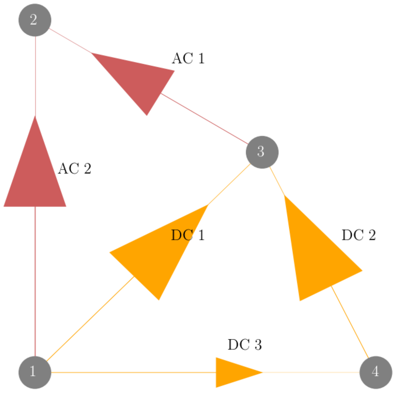
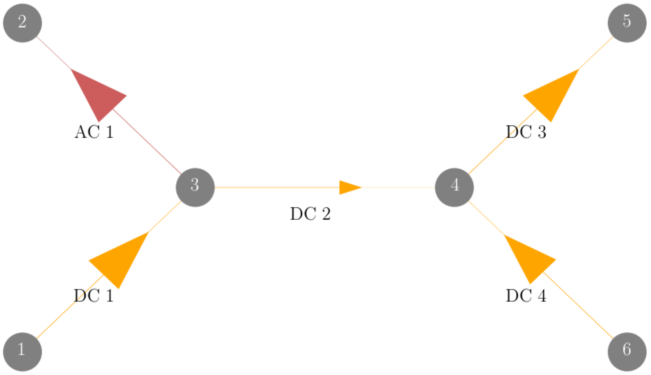
4. Flow Allocation across European Synchronous Zones

In the following, the formalism presented in Section 2 and Section 3 is applied to a highly renewable European network model in order to extract general sink-source relations and transmission flow behavior. We show how cross-border flows are mainly driven by wind power and transmission system usage derived from the MP algorithm is allocated to the countries.

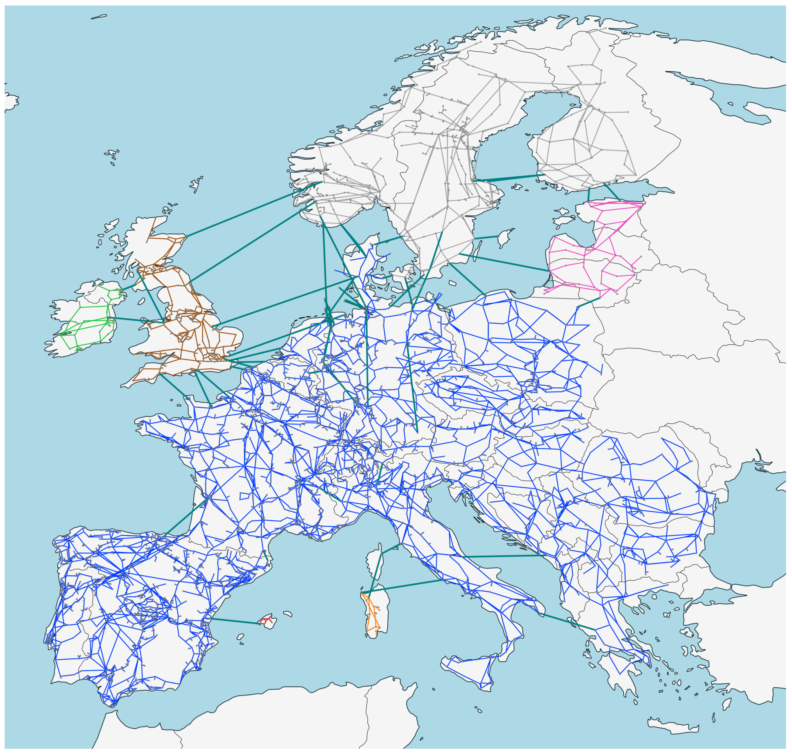
The European power system comprises five synchronous zones of heterogeneous sizes and covers the whole European Network of Transmission System Operators for Electricity (ENTSO-E) area. As displayed in Figure 3, these zones comprise the synchronous grid of Continental Europe (blue), representing the largest with 24 countries, the North of Europe (gray), the Baltic States (pink), the United Kingdom (brown), Ireland (light green), Mallorca (red), and Sardinia (orange). They are interconnected by HVDC lines in dark green. The data for the figure is retrieved from the interactive ENTSO-E transmission system map [18].

Each synchronous zone distributes power through AC lines and, in a nominal operational state, balances all loads within the subnetwork. The power flow on the passive AC lines are determined by the Kirchhoff current law and Kirchhoff voltage law and are in direct relation to the nodal power injection. Therefore, if the loading of passive branches is getting close to the capacity limits, Transmission System Operators (TSOs) have to regulate and reduce the critical power flows via redispatch. However, with upcoming HVDC projects realized within the Ten Year Network Development Plan (TYNDP) [19], additional controllable system elements will allow one to distribute power more efficiently.

The openly available power system model PyPSA-EUR, presented in [20] and available at [21], suits due to it’s realistic topology representing a realistic European meshed AC-DC network. The model itself is based on refined data of the European transmission system containing all substations and AC lines at and above 220 kV, all HVDC lines as well as most of today’s conventional generators. It is accessible via an automated software pipeline, which allows one to examine different scenarios, e.g., by varying transmission network expansion limits, CO${}_2$ caps or coupling of the heat, transport, and electricity sector as done by Brown et al. [22]. In order to represent a highly renewable future scenario, the network is clustered, simplified, and linearly cost-optimized, allowing generator expansion and 18% total transmission capacity expansion. Further, the CO${}_2$ cap is set to 5% of the 1990 emission level. Available generation technologies are onshore and offshore wind, solar PV, natural gas, and run-of-river.

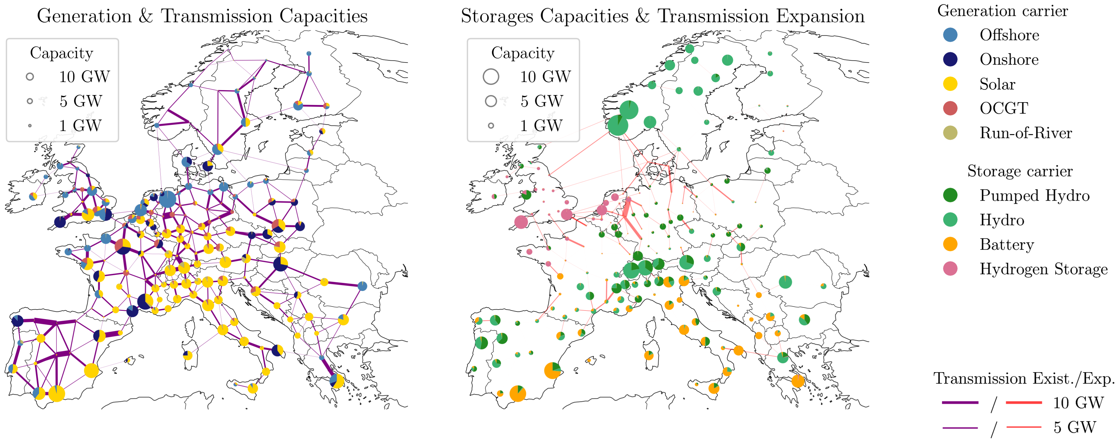
Available storage technologies are pumped-hydro-storage (PHS), hydro dams, batteries, and hydrogen storage. Note that hydro dams (hydro) do not have the ability to store power from the electricity grid, but are supplied by natural water inflow. All generator and storage types are allowed to be expanded except for PHS and hydro. Dispatch and expansion were calculated using the linear power flow approximation, neglecting line losses, and minimizing total system costs consisting of capital and operational expenditures of the different network components. The resulting network, shown in Figure 4, comprises N = 181 buses and L = 373 lines, of which 48 are controllable DC lines. The left hand side shows power generation and original transmission capacities, and the right side shows a capacity distribution of storage and transmission expansion. The energy production is strongly relying on wind power, which produces 40% of the yearly total of $3.13\times {10}^{15}$ Wh in offshore regions and 18% in onshore regions. Solar power on the other hand accounts for 23% of the total energy production. The rest is covered by hydro power (10%), open cycle gas turbines (5%), and run-of-river (4%). The average electricity price equals 58 €/MWh. The time-averaged total power flow in the transmission system is 316 GW. The spatial distribution of batteries correlates with the installation of solar power, most prominent in the European South. Hydrogen storage on the other hand is mostly distributed at wind power production centers along the North Sea coast. These technological “matches” result from the fact that batteries suit better for diurnal charging cycles, whereas hydrogen storage is rather cost-efficient for the long term and synoptic variability as experienced by wind power.

The FA analysis is done on the basis of the NetAllocation package, openly available at [23]. The two extended methods are applied on the whole simulation year, which consists of 2920 time steps representing a three-hour time resolution. We choose the standard formulation with $q=0.5$, where the difference between the MP and EBE algorithms are expected to be the largest. As the analysis of the three-dimensional data $\tilde{\mathbf{P}}\left(t\right)$ and $\tilde{\mathbf{F}}\left(t\right)$ requires detailed reporting, we want to restrict the analysis in the following to international power exchanges.

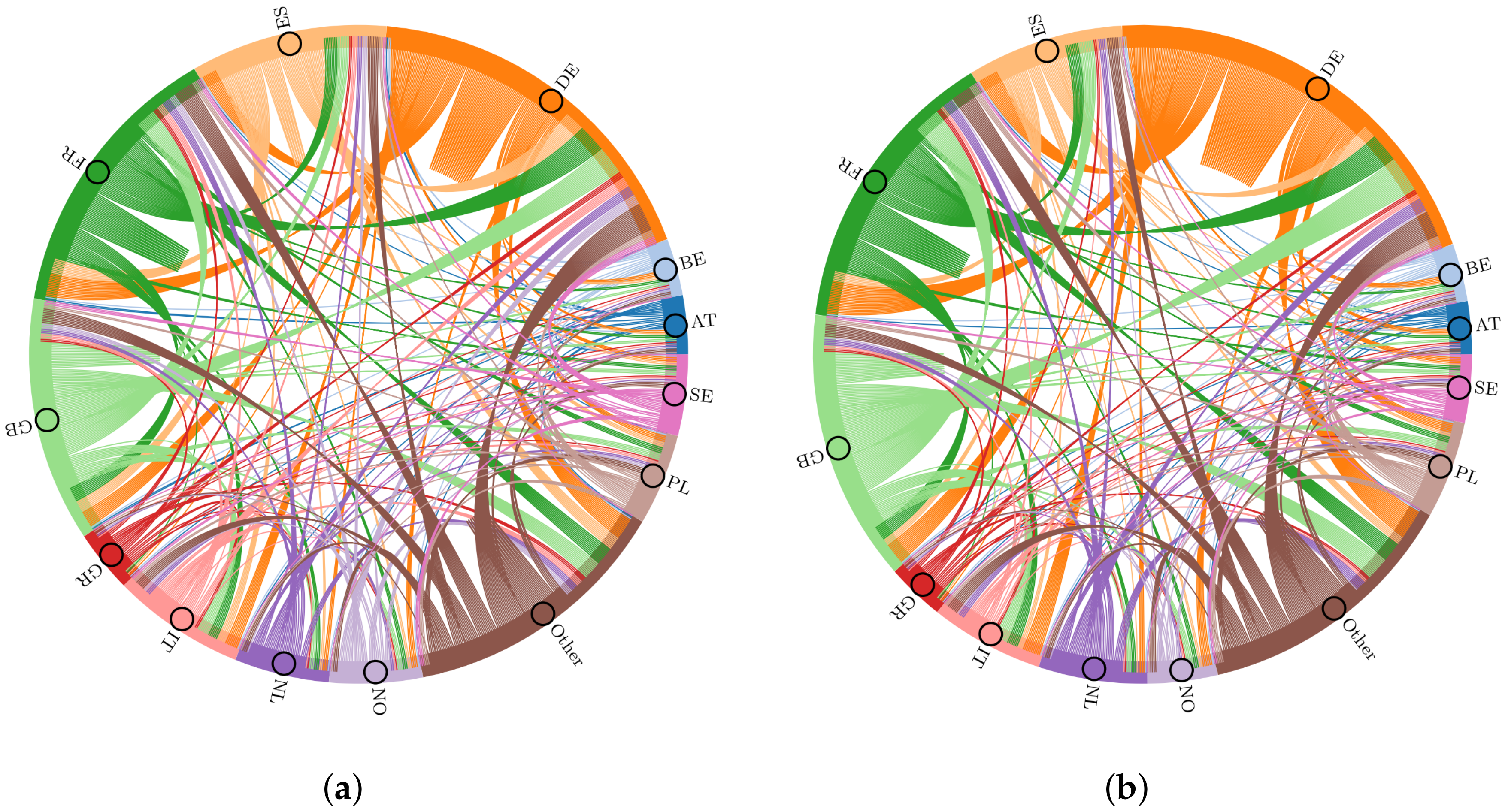
Figure 5a shows the average source-sink allocation, given by ${\mathbf{A}}_{\mathrm{MP}}={\mathbf{A}}_{\mathrm{EBE}}$, aggregated to countries. Colors of the outer circle indicate the overall exchange of the considered country. Colors of the inner circle and inbound connections represent either exports of the country (same color as the outer circle) or imports from other countries (corresponding colors of other countries in the outer circle). Self-assigned allocations are connections with the country itself, as one can clearly see, for instance, for Germany. The allocated cross border flows (CBF) are dominated by large exporters and importers in the system. Therefore, only 12 countries with the largest cross border exchange are represented separately, whereas the remaining countries are aggregated as “Other”. In the cost-optimized setup, Germany, France, and the United Kingdom are the strongest exporters and importers. However, there are countries with a much higher export-import ratio, such as Greece or Netherlands. Note that, by definition of the peer-to-peer relations for both methods, Equation (18) does not takes geographical distance into account and thus leads to large-distance exchanges, e.g., Germany–Spain or Finland–Italy. However, neighboring countries disclose the strongest interconnections. This applies particularly to countries along the North Sea coast where transmission expansion allows for strong interactions. Moreover, optimizing the cost of capacity expansion and disposition may lead to more installation and generation in regions near load centers. The FA methods now allow one to further break down the cross border flow allocation. Figure 5b shows the same setup but only includes power transfers induced by wind power injection. Remarkably, the country-to-country allocation hardly changes, as the overall CBF allocation is mainly driven by countries with strong wind production. Indeed, CBF induced by wind power covers 69% of the total CBF.

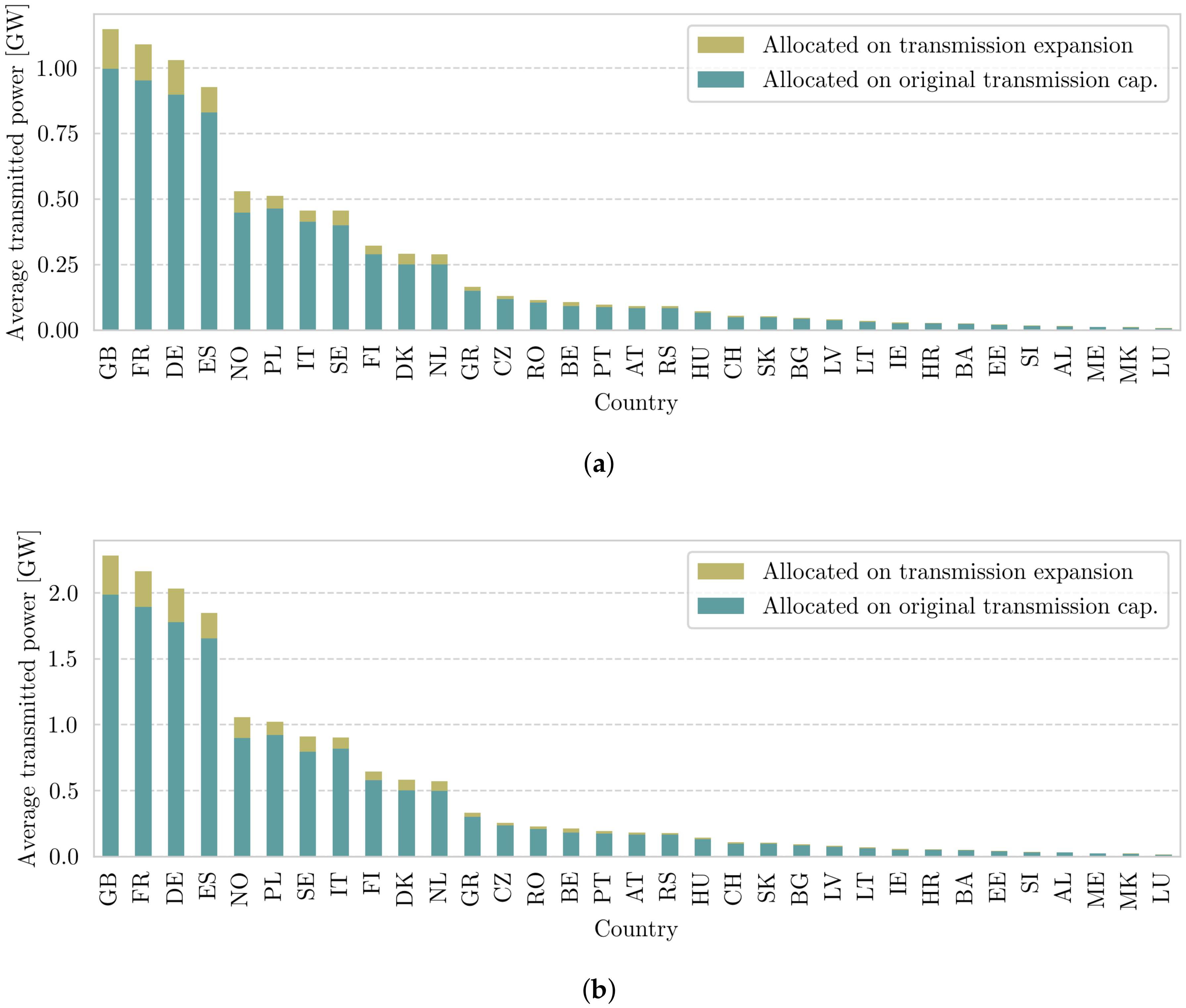
As the peer-to-peer relations are dominated by strong exporters of power, we want to have a look at the transmission grid usage, which is given by $\tilde{\mathbf{F}}$. Especially, the usage of the transmission expansion might be of current interest in regard to cost allocation of grid expansion projects. Therefore, we split the flow $\underline{\mathbf{f}}$ into two categories:

• a flow on a line stays within the bounds of today’s line capacities, or
• a flow exceeds the original transmission capacity and thus makes use of the 18% transmission expansion.

In Figure 6a,b, the average induced transmission for each country is shown. Each bar is split according to the two categories. First of all, it is remarkable how similar EBE and MP correlate on the aggregated country level. Despite strong absolute differences, the relative proportions are almost the same. The strongest transmission grid users are Great Britain, France, Germany, and Spain, followed by Norway after a large gap. More or less similar are the usages of transmission expansion distributed. Thus, even though Great Britain is not the strongest power exporter or importer, it has the highest average share of flows in the system. This indicates that, due to its topological situation and injection behavior, its power exports and imports are, on average, of longer spatial distance, which pushes the usage of the original and expanded transmission grid.

The transmission grid usage strongly anti-correlates with the amount of storage capacity. Thus, countries such as Italy that relate on high solar power shares and strong battery storage capacities, have a proportionally small dependence on the transmission grid. Thus, for a simplified approach of allocating capital and operational expenditures of the transmission grid to countries, one can legitimately propose to allocate capital expenditures proportional to the use of transmission expansion flow (the upper parts of the bars) and operational expenditures proportional to the flow allocation within the original capacity bound (lower parts).

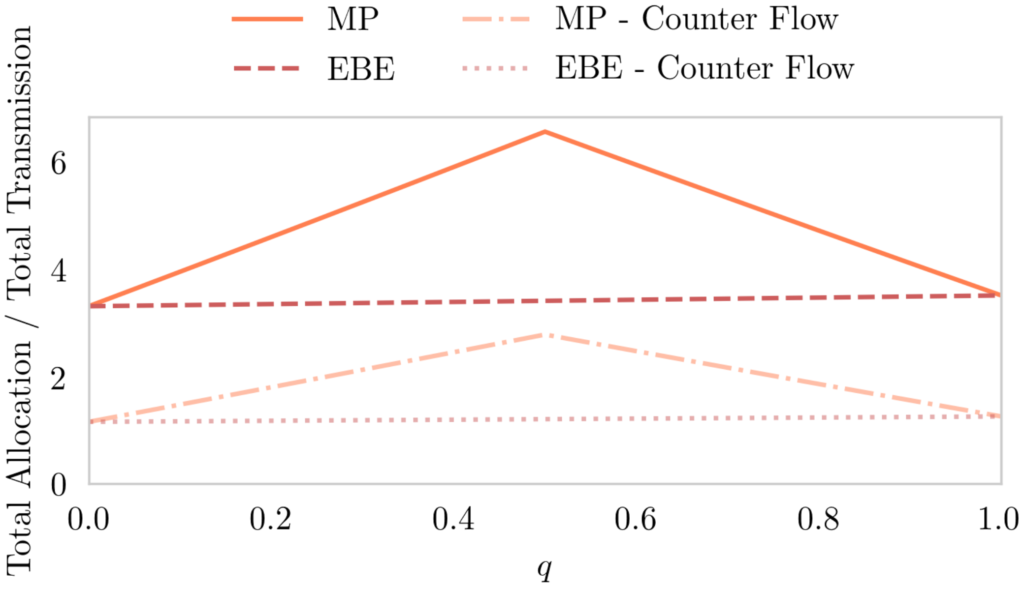
Finally, we close with a short discussion about higher absolute flow contributions in the MP allocation compared to EBEs. As pointed out earlier, with the 50–50% split, the MP algorithm leads to effective flows from net producer to net producer. This leads to higher shares of counter flows in the allocation, which on the other hand have to be balanced according to Equation 7. Figure 7 shows the ratio between the sum of absolute allocated flows and the total transmission as a function of q. Indeed, in the realm $0<q<1$, the MP method allocates much more flow, peaking at q = 0.5 with more than six times the total transmitted power, whereas the EBE method stays steadily at around three times the total transmission. The two lower lines reflect the sum of all allocated counter-flows which, as to expect, lays 0.5 below the half of the absolute allocation sums. In other words, each counter-flow cancels out with an aligned flow, and the remaining aligned flows sum up to $\underline{\mathbf{f}}$.

Note that it can be assumed that this effect scales with the network resolution, as the number of possible peer-to-peer connections scales with $\mathcal{O}\left(N^2\right)$. For $q=0.5$, ${\tilde{\mathbf{P}}}_{\mathrm{mp}}$ exploits all of these connections, which makes the appearance of counter-flows much more likely. However, further research needs to be done to sustain this argument.

5. Summary and Conclusions

A mathematical consistent extension of the Power Transfer Distribution Factor (PTDF) matrix that incorporates the operational state of controllable elements as high-voltage direct current lines was presented. By introducing a flow dependent pseudo-impedance vector $\overline{\mathit{\omega }}\left(\underline{\mathbf{f}}\right)$ of the size of controllable elements in the grid, the PTDF matrix was reformulated for meshed AC-DC networks. Thereby, it becomes essential to differentiate between the controllable elements being part of an independent cycle in the network or not, as both cases are affected by a different set of physical constraints. The extension was propagated to the reformulated and extended MP and EBE algorithm, which are both flow allocation methods based on the PTDF matrix. Thereby, both algorithms become applicable for meshed AC-DC networks and thus can be used, for instance, to analyze the European power system. On the basis of a future scenario model of the European power system, a flow allocation was performed to determine cross border transactions and transmission grid usage per country. It could be shown that FA methods can be appropriately used to quantify the usage of transmission expansion and opens a possible distribution scheme for capital expenditures on transmission projects.