Optimal Torque Distribution Control of Multi-Axle Electric Vehicles with In-wheel Motors Based on DDPG Algorithm


1
State Key Laboratory of Automotive Simulation and Control, Jilin University, Changchun 130022, China
2
College of Computer Science and Electronic Engineering, Hunan University, Changsha 410082, China
*
Author to whom correspondence should be addressed.
Energies 2020, 13(6), 1331; https://doi.org/10.3390/en13061331
Submission received: 7 February 2020
/
Revised: 8 March 2020
/
Accepted: 10 March 2020
/
Published: 13 March 2020
(This article belongs to the Special Issue Electric Systems for Transportation)
Abstract
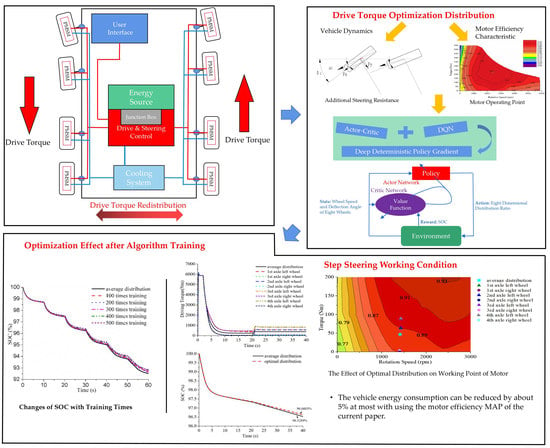
:In order to effectively reduce the energy consumption of the vehicle, an optimal torque distribution control for multi-axle electric vehicles (EVs) with in-wheel motors is proposed. By analyzing the steering dynamics, the formulas of additional steering resistance are given. Aiming at the multidimensional continuous system that cannot be solved by traditional optimization methods, the deep deterministic policy gradient (DDPG) algorithm for deep reinforcement learning is adopted. Each wheel speed and deflection angle are selected as the state, the distribution ratio of drive torque is the optimized action and the state of charge (SOC) is the reward. After completing a large number of training for vehicle model, the algorithm is verified under conventional steering and extreme steering conditions. The maximum SOC decline of the vehicle can be reduced by about 5% under conventional steering conditions based on the motor efficiency mapused. The combination of artificial intelligence technology and actual situation provides an innovative solution to the optimization problem of the multidimensional state input and the continuous action output related to vehicles or similar complex systems.
1. Introduction
The vehicles independently driven by in-wheel motors removes the transmission system of traditional vehicles and the drive torque of each wheel is independently controllable. Besides, the information such as the motor torque and speed can accurately feedback in real-time, so that the transmission efficiency of the vehicle is greatly improved and the layout design becomes more flexible. More importantly, the driving form has significant advantages in terms of stability control, active safety control and energy saving control [1,2], which is a huge attraction for multi-axle heavy vehicles. However, battery technology has always been one of the key issues limiting the development of pure electric vehicles [3]. For heavy vehicles, both the demand and consumption of energy are greater, which means the energy problem is more serious. In the case that the existing battery core technology cannot be solved temporarily, it is necessary to adopt an energy-saving control strategy for the electric vehicle, especially the multi-axle heavy-duty electric vehicle [4].
At present, the energy-saving driving control strategy for electric vehicles is mainly based on three aspects: motor control energy saving, energy feedback and traction control energy saving. The energy-saving of the motor is mainly based on the motor efficiency characteristic curve [5,6], aiming at the optimal system efficiency, and changing the actual working point of each motor by adjusting the front and rear axle torque distribution coefficients to avoid working in the low-efficiency zone, but this method is often only for straight-line driving conditions. Energy feedback mainly refers to regenerative braking technology, which hopes to maximize the recovery of braking energy by using different control strategies during vehicle braking [7,8,9]. In terms of traction control energy saving, the drive torque and braking torque of each wheel can be controlled independently for electric vehicles. By properly distributing the torque of each wheel, for example, taking the minimum sum of the tire utilization ratios of the driving wheels as the control target [10,11,12], so as to reduce the energy consumption rate or increase the power of the vehicle [13]. Generally, the optimization method is to turn the torque distribution formula according to vehicle dynamics into the parameter optimization problem under certain constraints [14,15,16]. However, this kind of method has great limitations in optimizing a multidimensional system.
At present, most of energy-saving control researches are aimed at the straight-line driving conditions evaluated by driving cycles [17] and there are relatively few studies on the vehicle energy-saving control for steering conditions. Compared with two-axle independent drive vehicles, only the two-dimensional optimal torque distribution control between the front and rear axles and between the left and right wheels is needed [18]. Multi-axle electric vehicles need to optimize the multidimensional independent space vector. Meanwhile, there are dynamic and kinematic connections between the wheels, which cannot be solved by traditional optimization algorithms.
The deep deterministic policy gradient (DDPG) [19,20] is an algorithm that improves on the basis of the deep Q network (DQN) [21,22] to solve continuous action problems. In reality, the vehicle is an extremely complex system, and the external environment is dynamic, complex and unknown, which means that it is difficult to simplify it into a fixed expression for quantitative analysis. The DDPG algorithm is highly adaptable and can be optimized for the black-box system in a dynamic environment, which is suitable for solving the practical problems of continuous action.
In the current paper, the four-axle (8 × 8) independent drive electric vehicle is taken as an example to study the torque distribution problem in the steering condition, and a 23-DOF (Degree of Freedom) vehicle dynamics model was built by MATLAB/Simulink (R2015a, MathWorks, Natick, MA, USA). After completing the relevant code of the DDPG algorithm, the data interaction between the algorithm and the vehicle model was realized, and the model was trained enough times through off-line simulation comparing energy consumption of the vehicle under the same conditions, so as to prove that the proposed control algorithm can effectively reduce energy consumption by reasonably distributing the drive torque of each wheel. Under the conventional steering condition and using the motor efficiency map of the current paper, energy consumption of the vehicle can be reduced by up to 5%.
2. Dynamics Model and Energy Analysis
2.1. Model Overview
As the number of axles increases, the dynamics of multi-axle vehicles becomes more complicated. Theoretically, the more the degrees of freedom of the vehicle are considered, the better the simulation effect will be, but the more parameters are actually required to be input, which will affect the results when relevant parameters cannot be obtained. In order to more accurately simulate the impact of vehicle systems and environment on the vehicle during driving, the classical 2-DOF linear model is not used in the vehicle dynamics model. Instead, based on the vehicle system dynamics theory, the differential equations of dynamics and kinematics are derived respectively about vehicle body, wheel and other systems. The suspension part is assumed to be static balance problem, and the tire part is analyzed by "Magic Formula". Finally, the related physical quantities between each system are used to connect the parts into a whole, as shown in Figure 1. Meanwhile, the way of modeling is also suitable for two-axle vehicles, and the simulation accuracy is higher. Based on the dynamics and kinematics equations of each system, the vehicle dynamics model is established by using MATLAB/Simulink. Taking into account 6-DOF of the vehicle body, including longitudinal, lateral, vertical, yaw, pitch, roll, as well as the vertical runout and rotation freedom of each wheel, and steering wheel angle, a total of 23-DOF. In addition, the vehicle adopts the steer-by-wire technology, which can realize all-wheel steering. In the model, according to the fixed relationship between the steering wheel angle and the deflection angle of the right wheel of the first axle and Ackerman steering principle, the S-Function module is built to calculate the actual deflection angle of each wheel, which is directly input into the vehicle dynamic model. The main parameters of the vehicle are shown in Table 1.
For electric vehicles with in-wheel motors, due to the complete decoupling of each wheel, in order to achieve electronic differential control, torque control mode is usually adopted for each in-wheel motor [23]. As shown in Figure 2, the drive control architecture is adopted. The total drive torque of the vehicle is obtained by the output of the PID (Proportion Integration Differentiation) controller, and the input of the controller is the deviation of the target speed and the actual speed. In general, the driving torque is evenly distributed to each wheel, so that the speed of wheel will follow according to its stress state. The average distribution mode can ensure the normal driving of vehicles, but it is not the optimal distribution method. Therefore, the optimal distribution mode of drive torque should be proposed, which is the main research content of the current paper.
2.2. Motor and Battery Model
As a high-speed rotating component, the speed characteristic of the motor also determines its high-speed response [24]. In general, the instantaneous response speed of the motor is tens of times faster than that of the wheel, so it can be simplified to a second-order response system [25], whose transfer function is as follows.
where Tmi is the actual input electromagnetic torque of each in-wheel motor, Tmi* is the desired input electromagnetic torque of each in-wheel motor, ξ denotes the damping ratio, which is related to the parameters of the drive motor. According to the response characteristics of PMSM, the value of ξ is 0.001.
At the same time, the motor efficiency map model is adopted. According to the speed and torque of the motor, the working efficiency can be obtained to calculate the corresponding energy loss. The efficiency map of the in-wheel motor used is shown in Figure 3.
For the battery model, in order to accurately compare the energy consumption, the ampere-hour integral method is adopted to estimate the battery SOC [26]. The formula is as follows.
where SOC0 is the initial state of charge and discharge, CN denotes the battery rated capacity, I is the instantaneous current of the battery, η represents the Coulomb efficiency coefficient, P is the actual working power of the battery, and U is the battery voltage. Generally, without considering the influence of temperature, the battery voltage will decrease with the decrease of SOC, but when the battery consumption is between 10% and 90%, the battery voltage variation is relatively small. In order to avoid the impact of the battery voltage change on the SOC drop, it is assumed that the battery consumption is always within this range, that is, the battery voltage remains constant.
2.3. Analysis of Steering Energy Consumption
When the vehicle enters the steering condition from the straight driving and the accelerator pedal opening is constant, the vehicle speed will decrease, which indicates that the vehicle driving resistance has increased. The movement of the vehicle is the result of the force from the ground to the vehicle body through the tire. Generally, the force between the tire and the ground is decomposed into longitudinal force and lateral force, and the motion of the vehicle is the result of the combined action. That is, the combined force of the longitudinal force and the lateral force causes the vehicle to generate steering motion. The direction of the resultant force is affected by factors such as drive torque, steering angle, and tire side-slip angle, and in the case of the same drive torque and steering angle, its direction is determined by the tire side-slip angle. When the vehicle turns, the tire force is shown in the Figure 4 below.
As shown in Figure 4, δ1 represents the wheel deflection angle, α is the tire side-slip angle, Fx and Fy denotes the tire longitudinal force and lateral force. Due to δ1 and α, the lateral force of the wheel will produce a reaction force along the longitudinal axis of the vehicle body, which increases the driving resistance. This explains why the speed of the vehicle will decrease when cornering and the opening of accelerator pedal remains the same, and it also means that if the vehicle wants to maintain the original speed, it needs to consume more energy. By establishing a single-track linear model and assuming that the vehicle moves in a uniform circular motion, the longitudinal force balance equation of the vehicle can be derived as follows.
where Fxi is the longitudinal force of each axle, Ff is rolling resistance, Fa denotes air resistance, m is the total mass of the vehicle, u represents the longitudinal velocity, ρ denotes the curvature radius, li is the horizontal distance from ith axle to the center of mass, L represents the distance between 1st axle and 4th axle, αi is the side-slip angle of ith axle. On the left side of the equation is the sum of longitudinal force of each axle and the first two terms on the right are the conventional driving resistance of vehicles. Therefore, the last term is the additional steering resistance caused by the tire slid-slip when the vehicle is steering [27,28], which denoted by Faf. If the drive torque of each wheel is changed, the drive force of the outboard wheels is increased and the drive force of the inboard wheels is decreased, then Equation (3) changes as follow.
where B is the wheel base, FΔ denotes the change in the drive force, δi is the deflection angles of the wheels. With other conditions unchanged, the smaller additional steering resistance, the smaller driving force required by the vehicle, and the less energy consumption. Then it can be seen from Equations (3) and (4) that under certain condition the increase of FΔ is conducive to the reduction of driving resistance. However, as it increases, the tire side-slip angle also increases, which will lead to the increase of the additional steering resistance, so it is not a monotonous change for the total driving resistance. Besides, the speed and deflection angles of wheels also affect the tire side-slip angle, so it is necessary to find the optimal torque distribution ratio at different speeds and steering angle, so as to make the driving resistance of the vehicle minimum.
In addition, the torque distribution of each wheel will also affect the actual working efficiency of the motor. Therefore, the total energy consumption of the vehicle should be taken as the optimization goal, and efficiency of all in-wheel motor is taken into account to achieve dynamic optimization.
3. The DDPG Algorithm
The deep deterministic policy gradient (DDPG) [29,30] is an improved algorithm based on DQN algorithm that can solve the problem of multidimensional continuous action output. This optimization method can operate for continuous action space, and it ignores the specific optimization model, which can complete the black-box learning, focusing on only three concepts [20]: state, action, and reward, and the goal is to get the most cumulative reward.
The selection of DDPG algorithm mainly considers the following points.
- (1)
- The research object of the current paper is the 8 × 8 independent drive electric vehicle, which is equivalent to operating an eight-dimensional independent space vector. It is far different from the two-dimensional optimization problem for 4WD vehicles. The DDPG algorithm is just able to optimize for the problem of multidimensional input and multidimensional continuous output.
- (2)
- The multi-axle vehicle system [31] is complex and difficult to simplify into a fixed expression, whereas DDPG algorithm is more adaptable and capable of learning and optimizing the black-box system.
- (3)
- The actual driving state of the vehicle is constantly changing. In addition to being influenced by the outside, the optimization action at each moment will affect the driving state of the vehicle at the next moment. DDPG algorithm is essentially a kind of reinforcement learning, which can adapt to interact and optimize in a dynamic environment to achieve a better state of adapting to the environment.
In the real word, there is an interaction process between the Agent and its surrounding dynamic environment [32], which can be explained as follows: after the Agent generates an action under a certain state, the environment will give the Agent corresponding reward, and then the Agent enters the next state and will generate the next action. Reinforcement learning is a machine learning model whose modeling goal is to construct the Agent in the environment so that the Agent can always generate actions in the environment to maximize reward. Considering the definition in reinforcement learning, the state of the Agent at time t is st, the action under state st is at, the feedback from the environment is rt, and the next state the agent enters is st+1. Corresponding to the content of the current paper, at time t, the vector (wt, δt) composed of the wheel speed (wt) and deflection angle (δt) of each wheel is regarded as st. The drive torque distribution ratio of each wheel (pt) can be regarded as at, the vehicle SOC (ut) can be regarded as rt. The vector (wt+1, δt+1) stands for st+1.
In reinforcement learning, the commonly used optimization objective (Rt) is the expectation of the total future reward at time t, which corresponds to the expectation of battery SOC in the future, as follows.
where γ is a coefficient, 0 < γ < 1, which makes sure that Rt convergence. In order to be able to solve Rt, the above formula can be rewritten as an iterative formula.
In the study of Q-learning, if we have the function to represent Rt, and then the optimal action strategy function can be obtained.
Usually as the environment is poorly understood, cannot be directly accessed but Deep Neural Network has been proved to be universal function approximator, so it can be used to approximate . In the current paper, Deep Neural Network is expressed as , where represents the parameter to be solved. In fact, the deep fully-connected neural network is used. Therefore, when approaches , is the optimal parameter , and the following equation can be obtained.
Due to the optimal action strategy function .
so the Equation (8) can be expressed as follows.
Therefore, the optimization objective of Deep Neural Network can be defined as follows.
where denotes the optimization objective function with as the independent variable. is expectation, and represents a probability distribution. The above equation is the optimization objective of DQN algorithm, but the optimization objective is only applicable when at is discrete. In the current paper, at is the multidimensional continuous space. So, considering an improved algorithm of DQN, DDPG uses Deep Neural Network to approximate the optimal action strategy function , so the optimization objective is as follows.
where represents DQN algorithm optimization target, denotes the optimization target of approximating the action strategy function . In order to make the optimization process more stable, and in the Equation (12) are replaced with and corresponding to the soft update parameters.
where τ is a coefficient, 0 < τ < 1. The expected calculation of and can be estimated approximately by Monte Carlo sampling, so the optimization objective is rewritten.
where N is the number of the dimension, N = 8, (i) denotes the corresponding wheel number. In fact, stochastic gradient descent algorithm is used to optimize the two optimization targets alternately, and the parameter update method is as follows.
When the optimal objective is reached, the parameters and are obtained, corresponding to Deep Neural Network and . The function can output a set of drive torque distribution ratio when the wheel speed and deflection angle are input in real time. The distribution ratio can make the expectation of SOC in the future maximum.
The network of at is called Actor network, then there are two networks in the algorithm, namely Rt-Q network and Actor network. Actor network is responsible for generating the action, which is the torque distribution ratio of each wheel. Rt-Q network is also commonly referred to as the Critic network, which is used to fit the sum of the system SOC for the next n steps, so that Actor network can have a clear optimization target. When the overall algorithm is executed, according to the training logic, in the Q network is updated first, and then as a parameter is input to the Actor network to update , with the aim of minimizing −Q. The actual training process is to train and in the two networks, and this process is called joint alternation training.
The overall implementation of architecture design is shown in Figure 5. The DDPG algorithm is directly embedded into the vehicle dynamics model by MATLAB Function to ensure real-time interaction. During the training process, the vehicle system outputs state and reward in real time. A total of 16-dimensional state signal is input to the Actor-network, including eight-dimensional wheel speed and eight-dimensional wheel deflection angle signals, and eight-dimensional wheel torque distribution ratio signal is output. For the Critic network, the same 16-dimensional state signal and eight-dimensional action signal output by the Actor-network are taken as the input to fit the sum of the energy consumption in the next n steps. In addition, the Train function is completed, which contains the logic of the algorithm training process, so that the Actor network and Critic network can update alternately according to the algorithm and complete the corresponding output.
In order to avoid the possible problems of data interaction between the two networks and Train function due to the synchronization of update in the model, all of them are written in a MATLAB Function module and directly called internally. At the same time, taking into account the actual passing ability of the vehicle, and preventing the long-term high torque output of individual motors to reduce the service life, the additional limitation is that the single-axle drive is not allowed in straight-line driving, with the 1st axle and 3rd axle as the main power distribution axle.
In addition, it needs to be clarified that the difference between the application scenario of the current paper and that of the traditional neural network algorithm is that the current action will directly affect the environment at the next moment. If the environment cannot be changed, actually only one step in the overall process is optimized.
4. Offline Simulation Verification
After the relevant algorithm code is completed and can interact with the vehicle model, the model needs to be trained for a certain number of times first. The purpose is to make the Actor and Critic network update their internal parameters according to the training logic of Train function to adapt to the whole system.
At present, there is no standard cycle condition for the evaluation of vehicle steering energy consumption, which results in the training condition of the model needs to be designed artificially. Different training conditions will affect the final optimization results of the model. The designed training condition should contain enough state samples of the optimized system. At the same time, it should be avoided that due to the influence of training environment, experience with certain type characteristics is particularly abundant, while experience with other type is scarce. At best, experience should have difference and similar experience should be minimized. During neural network training, some unexpected changes are not considered in the current paper, because they are difficult to be included completely. However, in order to avoid related problems, the average distribution as a conservative control scheme was combined with the neural network. By comparing the reward at any time, the control scheme with a higher reward is adopted, so as to ensure that the energy consumption of the vehicle was not lower than the conventional driving mode under any working condition, which is a supportability control strategy.
The state variables in the algorithm are the wheel speed and the wheel deflection angle. Therefore, based on the above principles, the model input of target vehicle speed and steering wheel angle are shown in Figure 6. During training, only the first and second axles were steering axles. Meanwhile, considering the stability problem of the vehicle in high speed, the amplitude of the steering angle decreased after 40 seconds.
According to the training conditions, after completing about 100, 200, ..., 500 times training, data and driving state curves were recorded. Figure 7a shows the change process of vehicle speed after different training times. The change of vehicle speed was little affected by the drive torque distribution and the target vehicle speed could be well followed. Since the optimal torque distribution is equivalent to applying an additional yaw moment for the vehicle, so the yaw rate of the vehicle was increased in each period after distributing, which can be seen in Figure 7b, and it is in line with the actual situation. Figure 7c is a comparison of the SOC change after the corresponding training number. It can be seen that the SOC decline decreased with the increase of training times. After 500 times of training, the SOC decline of this training condition was reduced by about 4.5320%.
After completing the training, only the parameter matrix in the Actor network is retained and stored into the MATLAB Function, which receive the driving state of the vehicle in real-time and generate the optimal distributing action. In theory, the more training times, the more stable and optimal parameters in the Actor network tend to be, and the better the optimization effect will be. However, with the increase of training times, the rate of optimization return is decreased. Meanwhile, in order to ensure the optimal effect, a fixed simulation step size of 1 millisecond was adopted in the Simulink, while the action was updated every 10 steps by the control algorithm, which led to a significant increase in the computational burden of the model. After completing 400 and 500 times training, and comparing the simulation results, it can be found that the optimization effect was almost the same. Therefore, considering the optimization efficiency, finally the model training was completed for 500 times.
4.1. Conventional Low-Speed Step Steering Condition
The low-speed simulation condition was designed to accelerate the vehicle from the stationary state with a target speed of 30 km/h. At the 20 s, the steering wheel turned about 230° within 1 s, and only the first and second axles were steering axles. Figure 8a shows the actual change in speed of vehicle. It can be seen that after the steering angle change, the vehicle speed decreased slightly, which was caused by the increase of driving resistance. It is consistent with the actual situation. Figure 8b is a detail view of vehicle speed. Compared with the average distribution, the steady-state vehicle speed increased slightly after the optimal distribution of drive torque, but the difference was not significant. Because the redistribution of drive torque led to the reduction of additional steering resistance, the drive torque required to maintain steady state was reduced. It can be seen from Figure 2 that under the condition that the target vehicle speed remained unchanged, the actual vehicle speed increased.
Figure 9 shows vehicle yaw rate change and the vehicle track comparison respectively. After optimization control, the yaw rate of the vehicle increased by around 1.02%, and the radius of the track was also slightly reduced. From Figure 8 and Figure 9, it can be seen that optimal torque distribution promoted the steering trend, but the influence on the various driving state parameters of the vehicle was not significant, and did not cause the stability problem.
It can be seen from Figure 10a that after adopting torque optimization control, SOC decline was significantly reduced and the energy consumption was reduced by about 3.7856% between 0 s and 40 s. However, it included the linear acceleration phase, although the torque was also optimally distributed during straight-line driving, the motor basically worked on the external characteristic curve during acceleration. At the same time, there was no training for the straight-line driving condition, so the optimization effect was not obvious. Then only for the steering phase between 20 s and 40 s, the vehicle energy consumption can be reduced by about 5.112% after optimization.
Figure 10b shows the change of the drive torque of each wheel. In the linear acceleration phase, the drive torque of the whole vehicle was mainly distributed to 1st axle and 3rd axle, similar to the two-axle drive, which increased the working load of some drive motors and improved overall work efficiency. When steering, the drive torque of the outboard wheel increased, and the drive torque of the inboard wheel decreased. Besides, the drive torque of rear axle of the outboard wheel was relatively larger, because in the same cases, the change of the drive torque of the rear axle had a greater influence on the additional yaw of the whole vehicle, which is more conducive to the reduction of the energy consumption. In addition, the multi-axle vehicle body is longer, resulting in the effect is relatively more obvious. When the vehicle was in steady-state steering, the driving torque of the whole vehicle is about 3107 Nm by average distribution, while the total driving torque is about 2975.4 Nm by optimized distribution, which is relatively reduced by about 4.2356%. Another part of the reduction in energy consumption comes from the improvement of motor working efficiency.
Figure 11 shows the comparison of working point change in the motor efficiency map. The wheel speed and output torque during steady-state steering are respectively derived. Based on the deceleration ratio, the actual working points of each in-wheel motor were calculated. As the relative speed difference between the left and the right wheel was very small, which can be approximately ignored, a point was used to represent the actual working point of each motor when the drive torque was evenly distributed. After the optimal torque distribution control was adopted, the actual working point of each motor was changed. The drive torque of the outboard wheel was increased, and the working efficiency was improved. Though the working efficiency of inboard wheel reduced, its drive torque was small, which led to the overall working efficiency being improved.
4.2. Conventional High-speed Sinusoidal Steering Condition
The high-speed simulation condition was designed to accelerate the vehicle from the stationary state with a target speed of 70 km/h. At 20 s, the steering wheel input a sine wave with an amplitude of 110° as shown in Figure 12a. Similarly, 1st axle and 2nd axle were steering axles. Figure 12b,c show changes of the vehicle speed and the yaw rate. Similar to the step steering condition, the change of driving state was not obvious and the peak of yaw rate increased slightly. Figure 12d shows the change of drive torque. Due to the input of the steering wheel constantly changing, the curvature radius of the vehicle driving was also changing. It can be seen from Equation (3) that the additional steering resistance fluctuated accordingly. Therefore, when the driving torque was evenly distributed, the driving torque of each wheel also changed correspondingly. After optimized distribution, the more drive torque was distributed to the wheel of the outboard and rear axles, which promoted the steering of the vehicle. Under the dynamic steering condition, the driving torque of each wheel could follow the changes of system input, which indicates that the optimal control algorithm could adapt to the dynamic environment.
The changes of SOC can be seen from Figure 13a. After the optimization control, the SOC decline reduced by 2.6213% between 0 s and 40 s. If only comparing the SOC change during steering phase, the energy consumption of the vehicle decreased by 4.0482% after optimization as shown in Figure 13b. It was proved that the optimal torque distribution control based on energy consumption could reasonably distribute the drive torque of each wheel and reduce the energy consumption under the dynamic condition. That means the optimization algorithm adopted was not limited to specific working conditions, which can be for any steering conditions, whether static or dynamic. The optimization algorithm could optimize the distribution of driving torque in real time and reduce the vehicle energy consumption. However, the optimization effect was slightly worse than that of low speed test, which was mainly for two reasons. On the one hand, the sine wave input was a dynamic process all the time, but there had to be system inertia in the mechanical system, which may have led to the actual action and control signals not being completely synchronized. Although the effect was relatively small for the electric vehicle with in-wheel motor, it could not guarantee that the drive torque of each wheel was optimal at any time; on the other hand, when the motor worked at a high speed, the high efficiency area on the efficiency map was relatively large, so the optimization effect after the control was slightly lower.
4.3. Extreme Steering Condition
In order to further reflect the control effect of optimal torque distribution, the extreme steering condition test was carried out. The four-axle reverse phase steering mode was adopted, with the first and second axles deflecting in the opposite direction to the third and fourth axles. The target speed of the vehicle was set to 10 km/h. At 20 s, the right wheel of the first axle deflected about 23° within 2 s, and the deflection angles of other wheels were calculated according to Ackerman steering principle, as shown in Figure 14a. For the change of speed, the vehicle speed after optimal control was still slightly higher than that under average distribution as shown in Figure 14b, which was the same as the previous simulation results. However, when the vehicle was in steady-state steering, the vehicle speed was basically unchanged compared with driving in the straight line, which indicates that the additional steering resistance was relatively small in this working condition.
As shown in Figure 15, the driving track of the vehicle remained unchanged basically after optimization. The steering radii of the vehicle after average distribution and optimal distribution were 8.1165 m and 8.1053 m respectively, which means that the optimal distribution of drive torque control did not have a great impact on the vehicle trajectory and body posture.
Figure 16 shows the change of wheel drive torque. 0 s to 20 s was a linear acceleration phase, and the drive torque was distributed between the axles. Since the motor was in the state of low speed and low torque at this stage, in order to improve the overall working efficiency, the driving torque of the vehicle was mainly distributed to the first axle and the third axle to increase the workload of the motor. When entering the steering at 20 s, due to the increase of the driving resistance, the driving torque of the vehicle increased in order to maintain the target speed. However, when the vehicle was in steady-state steering, the drive torque was basically the same as that when the vehicle traveled in a straight line, which was caused by the reduction of driving resistance by the four-axle reverse phase steering. It can be seen that the optimization control made the distribution ratio of the outboard and rear axle wheels increase, which further promoted the reduction of driving resistance, thus achieving the purpose of reducing the driving energy consumption.
When the vehicle was in steady-state steering, the total required drive torque of the vehicle with the average torque distribution was 1860.0376 Nm, and after the optimal distribution control, it was only 1656.6745 Nm, which was about 10.9332% lower. Then the change of the vehicle SOC during the steering phase was compared. The actual energy consumption decreased by about 13.3679%, which was much more obvious than the conclusion obtained by the above that maximum reduction in energy consumption is about 5%. This is mainly because the working efficiency of the motor is extremely low under low speed conditions [33]. Meanwhile, according to the motor efficiency map used in this paper, when the vehicle speed was lower than 30 km/h, the efficiency changed greatly with the torque, so the optimization control effect was better under this working condition. Besides, it was found that when other conditions were the same and four-axle reverse phase steering was adopted, the vehicle demand torque was far less than that when two-axle steering was adopted, sometimes less than half of that. Smaller drive torque led to lower working efficiency, which also led to the more obvious optimization effect.
4.4. Performance Evaluation
It should be emphasized that the optimal distribution of drive torque control can achieve the maximum energy saving effect of about 5% in the conventional steering conditions, but it is only for the motor efficiency map used in the current paper (Figure 3). The motor efficiency map had a great influence on the actual optimization effect. If the high efficiency area of the in-wheel motor was small, the energy saving control effect on the vehicle was obvious. In addition, the selection of algorithm training conditions should be closer to the actual driving state of the vehicle, and enough training times should be ensured to make the parameters in the Actor network tend to the stable and optimal value.
5. Conclusions
- (1)
- Based on the theory of vehicle system dynamics, the dynamic model of an 8 × 8 independent drive electric vehicle is built by MATLAB/Simulink, which contains 23-DOF to more accurately describe the multi-axle vehicle dynamics. On the basis, combining with the analysis of tire force and the mathematical derivation of the single-track linear model, it is concluded that through the reasonable distribution of the driving torque can reduce the additional steering resistance, and then reduce the energy consumption of the vehicle. However, due to the change of the tire side-slip angle and the influence of the motor efficiency, the optimization process is necessarily dynamic.
- (2)
- Considering the research object and content of the current paper, the DDPG algorithm is adopted to optimize the distribution of the drive torque between each wheel to reduce the energy consumption of the vehicle. The formula of DDPG algorithm is derived, and the overall system architecture is designed. The Actor network, Critic network and Train function are completed to interact with the vehicle model with the help of MATLAB Function, and realize the joint alternation training.
- (3)
- Since there is no standard for the evaluation of steering energy consumption, the training condition is designed artificially. After completing 500 times training, the parameter matrix in the Actor-network is stored into the MATLAB Function, which receive the driving state of the vehicle in real-time and generate the optimal distributing action. The low speed, high speed conventional steering and extreme steering simulation tests are carried out respectively. The results show that the vehicle energy consumption can be reduced by about 5% at most under the conventional steering condition with using the motor efficiency map of the current paper, which effectively reduces the energy consumption for the multi-axle electric vehicles with in-wheel motors. Meanwhile, the current paper provides an innovative solution to the vehicle optimization problem of multidimensional state input and multidimensional continuous output.
Author Contributions
Conceptualization, Q.Z. and D.T.; methodology, L.J.; software, D.T. and J.W.; validation, D.T. and L.J.; formal analysis, D.T. and Q.Z.; investigation, D.T.; resources, J.W.; data curation, D.T.; writing—original draft preparation, L.J.; writing—review and editing, D.T., Q.Z. and J.W.; visualization, D.T.; supervision, L.J.; project administration, L.J.; funding acquisition, D.T. All authors have read and agreed to the published version of the manuscript.
Funding
This research was funded by Natural Science Foundation of Jilin Province (Grant No.: 20170101208JC).
Conflicts of Interest
The authors declare no conflict of interest. The funders had no role in the design of the study; in the collection, analyses, or interpretation of data; in the writing of the manuscript, or in the decision to publish the results.
References
- Chan, C.C.; Chau, K.T. Modern Electric Vehicle Technology. Power Eng. 2001, 16, 240. [Google Scholar]
- Hou, R.F.; Zhai, L.; Sun, T.M.; Hou, Y.H.; Hu, G.X. Steering Stability Control of a Four In-Wheel Motor Drive Electric Vehicle on a Road with Varying Adhesion Coefficient. IEEE Access 2019, 7, 32617–32627. [Google Scholar] [CrossRef]
- Ehsani, M.; Gao, Y.M.; Emadi, A. Modern Electric, Hybrid Electric, and Fuel Cell Vehicles: Fundamentals, Theory and Design, 2nd ed.; CRC Press: New York, NY, USA, 2009. [Google Scholar]
- Tang, B. Application prospect of heavy-duty multi-axle special transportation vehicle. Automob. Parts 2012, 48, 30–33. [Google Scholar]
- Kim, J. Optimal power distribution of front and rear motors for minimizing energy consumption of 4-wheel-drive electric vehicles. Int. J. Automot. Technol. 2016, 17, 319–326. [Google Scholar] [CrossRef]
- Qian, H.H.; Xu, G.Q.; Yan, J.Y.; Lam, T.L.; Xu, Y.; Xu, K. Energy Management for Four-Wheel Independent Driving Vehicle. In Proceedings of the IEEE/RSJ International Conference on Intelligent Robots and System, Taipei, Taiwan, 18–22 October 2010. [Google Scholar]
- Gao, T.M.; Chu, L.; Ehsani, M. Design and Control Principles of Hybrid Braking System for EV, HEV and FCV. In Proceedings of the 2007 IEEE Vehicle Power and Propulsion Conference, Arlington, TX, USA, 9–12 September 2007; pp. 384–391. [Google Scholar]
- Li, N.; Zhang, J.Z.; Zhang, S.Y.; Hou, X.; Liu, Y. The influence of accessory energy consumption on evaluation method of braking energy recovery contribution rate. Energy Convers. Manag. 2018, 166, 545–555. [Google Scholar] [CrossRef]
- Chen, Y.; Wang, J.M. Fast and Global Optimal Energy-Efficient Control Allocation with Applications to Over-Actuated Electric Ground Vehicles. IEEE Trans. Control Syst. Technol. 2012, 20, 1202–1211. [Google Scholar] [CrossRef]
- Lenzo, B.; Bucchi, F.; Sorniotti, A.; Frendo, F. On the handling performance of a vehicle with different front-to-rear wheel torque distributions. Veh. Dyn. Syst. 2018, 57, 1685–1704. [Google Scholar] [CrossRef]
- Yamakawa, J.; Watanabe, K. A method of optimal wheel torque determination for independent wheel drive vehicles. J. Terramech. 2006, 43, 269–285. [Google Scholar] [CrossRef]
- Mokhiamar, O.; Abe, M. Simultaneous Optimal Distribution of Lateral and Longitudinal Tire Forces for the Model Following Control. J. Dyn. Syst. Meas. Control 2004, 126, 753–763. [Google Scholar] [CrossRef]
- Park, J.; Jeong, H.; Jang, I.G.; Hwang, S.H. Torque Distribution Algorithm for an Independently Driven Electric Vehicle Using a Fuzzy Control Method. Energies 2015, 8, 8537–8561. [Google Scholar] [CrossRef]
- Dizqah, M.A.; Lenzo, B.; Sorniotti, A.; Gruber, P.; Fallah, S.; De Smet, J. A Fast and Parametric Torque Distribution Strategy for Four-Wheel-Drive Energy-Efficient Electric Vehicles. IEEE Trans. Ind. Electron. 2016, 63, 4367–4376. [Google Scholar] [CrossRef] [Green Version]
- Yu, Z.P.; Zhang, L.J.; Xiong, L. Optimized Torque Distribution Control to Achieve Higher Fuel Economy of 4WD Electric Vehicle with Four In-Wheel Motors. J. Tongji Univ. 2005, 33, 1355–1361. [Google Scholar]
- Fan, J.J.; Mao, M. A Study of Driving Force Distribution Strategy for Three-axles Electric Driving Vehicle Based on Economics. Veh. Power Technol. 2007, 1, 52–59. [Google Scholar]
- Li, B.; Goodarzi, A.; Khajepour, A.; Chen, S.K.; Litkouhi, B. An optimal torque distribution control strategy for four-independent wheel drive electric vehicles. Veh. Syst. Dyn. 2015, 53, 1172–1189. [Google Scholar] [CrossRef]
- Jing, H.H.; Jia, F.J.; Liu, Z.Y. Multi-Objective Optimal Control Allocation for an Over-Actuated Electric Vehicle. IEEE Access 2018, 6, 4824–4833. [Google Scholar] [CrossRef]
- Mnih, V.; Kavukcuoglu, K.; Silver, D.; Graves, A.; Antonoglou, I.; Wierstra, D.; Riedmiller, M. Playing Atari with Deep Reinforcement Learning. Comput. Sci. 2013, arXiv:1312.5602. [Google Scholar]
- Lillicrap, T.P.; Hunt, J.J.; Pritzel, A.; Heess, N.; Erez, T.; Tassa, Y.; Silver, D.; Wierstra, D. Continuous control with deep reinforcement learning. Comput. Sci. 2015, 8, 187–200. [Google Scholar]
- Mnih, V.; Kavukcuoglu, K.; Silver, D.; Rusu, A.A.; Veness, J.; Bellemare, M.G.; Graves, A.; Riedmiller, M.; Fidjeland, A.K.; Ostrovski, G.; et al. Human-level control through deep reinforcement learning. Nature 2015, 518, 529–533. [Google Scholar] [CrossRef]
- Silver, D.; Lever, G.; Heess, N.; Degris, T.; Wierstra, D.; Riedmiller, M. Deterministic policy gradient algorithms. In Proceedings of the International Conference on International Conference on Machine Learning, Beijing, China, 21–26 June 2014; pp. 387–395. [Google Scholar]
- Jin, L.Q.; Wang, Q.N.; Zhang, H.H.; Wang, J.N. A Study on Differential Technology of In-wheel Motor Drive EV. Automot. Eng. 2007, 29, 700–704. [Google Scholar]
- Tursini, M.; Parasiliti, F.; Zhang, D.Q. Real-time gain tuning of PI controllers for high-performance PMSM drives. IEEE Trans. Ind. Appl. 2002, 38, 1018–1026. [Google Scholar] [CrossRef]
- Harris, T.A.; Kotalas, M.N. Rolling Bearing Analysis; CRC Press: Boca Raton, FL, USA, 2010; pp. 124–132. [Google Scholar]
- Li, Z.; Lu, L.G.; Ouyang, M.G. Comparison of Methods for Improving SOC Estimation Accuracy through an Ampere-hour Integration Approach. J. Tsinghua Univ. (Sci. Technol.) 2010, 8, 2193–2196. [Google Scholar]
- Zhang, H.H. Research on the Torque Coordinating Control of In-Wheel Motor Driving Electric Vehicle. Ph.D. Thesis, Auto-Body Engineering Department of College of Automobile Engineering of Jilin University, Changchun, China, 2009. [Google Scholar]
- Sun, W.; Wang, Q.N.; Wang, J.N. Yaw-moment control of motorized vehicle for energy conservation during cornering. J. Jilin Univ. (Eng. Technol. Ed.) 2018, 48, 11–19. [Google Scholar]
- Kim, S.J.; Kim, H.S.; Kang, D.J. Vibration Control of a Vehicle Active Suspension System Using a DDPG Algorithm. In Proceedings of the IEEE International Conference on Control, Automation and Systems (ICCAS), Daegwallyeong, Korea, 17–20 October 2018. [Google Scholar]
- Hou, J.; Li, H.; Hu, J.W.; Zhao, C.; Guo, Y.; Li, S.; Pan, Q. A review of the applications and hotspots of reinforcement learning. In Proceedings of the 2017 IEEE International Conference on Unmanned Systems (ICUS), Beijing, China, 27–29 October 2017. [Google Scholar]
- Du, H.; Wang, Z.B.; Wang, Y.; Huang, H. Adaptive Robust Control of Multi-Axle Vehicle Electro-Hydraulic Power Steering System with Uncertain Tire Steering Resistance Moment. IEEE Access 2018, 7, 5519–5530. [Google Scholar] [CrossRef]
- Xu, X.; He, H.G. A Gradient Algorithm for Neural-Network-Based Reinforcement Learning. Chin. J. Comput. 2003, 26, 227–233. [Google Scholar]
- Gu, C.; Liu, H.; Chen, X.B. Torque Distribution Based on Efficiency Optimization of Four-wheel Independent Drive Electric Vehicle. J. Tongji Univ. (Nat. Sci.) 2015, 43, 1550–1556. [Google Scholar]
Figure 1.
Vehicle dynamics model architecture.

Figure 2.
Vehicle drive control.

Figure 3.
Drive motor efficiency map.

Figure 4.
Tire force decomposition diagram.

Figure 5.
Training process architecture of deep deterministic policy gradient (DDPG) algorithm.

Figure 6.
Model input of the training condition: (a) target vehicle speed; (b) steering wheel angle.
Figure 6.
Model input of the training condition: (a) target vehicle speed; (b) steering wheel angle.

Figure 7.
Changes of vehicle driving parameters and battery state of charge (SOC) after training: (a). Changes of vehicle speed with training times; (b). Changes of yaw rate with training times; (c). Changes of SOC with training times.
Figure 7.
Changes of vehicle driving parameters and battery state of charge (SOC) after training: (a). Changes of vehicle speed with training times; (b). Changes of yaw rate with training times; (c). Changes of SOC with training times.


Figure 8.
Changes of vehicle speed during low-speed simulation: (a). Changes of vehicle speed; (b). Partial enlarged drawing.
Figure 8.
Changes of vehicle speed during low-speed simulation: (a). Changes of vehicle speed; (b). Partial enlarged drawing.

Figure 9.
Vehicle yaw rate change and the vehicle track comparison: (a). Changes of yaw rate; (b). Comparison of driving trajectory.
Figure 9.
Vehicle yaw rate change and the vehicle track comparison: (a). Changes of yaw rate; (b). Comparison of driving trajectory.

Figure 10.
Changes of vehicle SOC and wheel drive torque after optimization: (a). Changes of vehicle SOC; (b). Changes of wheel drive torque.
Figure 10.
Changes of vehicle SOC and wheel drive torque after optimization: (a). Changes of vehicle SOC; (b). Changes of wheel drive torque.

Figure 11.
Comparison of motor working points.

Figure 12.
Changes in vehicle driving parameters during high-speed simulation condition: (a). Steering wheel angle; (b). Vehicle speed; (c). Yaw rate; (d). Drive torque of each wheel.
Figure 12.
Changes in vehicle driving parameters during high-speed simulation condition: (a). Steering wheel angle; (b). Vehicle speed; (c). Yaw rate; (d). Drive torque of each wheel.


Figure 13.
Changes of SOC after the optimization control: (a). Changes of SOC in the whole process; (b). Changes of SOC in the steering phase.
Figure 13.
Changes of SOC after the optimization control: (a). Changes of SOC in the whole process; (b). Changes of SOC in the steering phase.

Figure 14.
Changes in vehicle driving parameters after the optimization control in reverse phase steering condition: (a) wheel deflection angle; (b) longitudinal vehicle speed.
Figure 14.
Changes in vehicle driving parameters after the optimization control in reverse phase steering condition: (a) wheel deflection angle; (b) longitudinal vehicle speed.

Figure 15.
Comparison of vehicle trajectory and body posture under average distribution and optimal distribution.
Figure 15.
Comparison of vehicle trajectory and body posture under average distribution and optimal distribution.

Figure 16.
Comparison of wheel drive torque change under average distribution and optimal distribution.
Figure 16.
Comparison of wheel drive torque change under average distribution and optimal distribution.


Table 1.
Main parameters of the whole vehicle.
| Basic Parameters | Value |
|---|---|
| Total mass of the vehicle (kg) | 25,000 |
| Height of the mass (m) | 1.20 |
| Wheel rolling radius (m) | 0.59 |
| The angle relationship between the steering wheel and the right wheel of the first axle | 20:1 |
| 1st axle and 2nd axle wheelbase L1 (m) | 1.42 |
| 2nd axle and 3rd axle wheelbase L2 (m) | 2.00 |
| 3rd axle and 4st axle wheelbase L3 (m) | 1.42 |
| Wheel center distance(m) | 2.60 |
| Drive reduction ratio | 10.8 |
| Battery rated capacity CN (Ah) | 120 |
| Battery voltage U (V) | 900 |
© 2020 by the authors. Licensee MDPI, Basel, Switzerland. This article is an open access article distributed under the terms and conditions of the Creative Commons Attribution (CC BY) license (http://creativecommons.org/licenses/by/4.0/).
Share and Cite
MDPI and ACS Style
Jin, L.; Tian, D.; Zhang, Q.; Wang, J. Optimal Torque Distribution Control of Multi-Axle Electric Vehicles with In-wheel Motors Based on DDPG Algorithm. Energies 2020, 13, 1331. https://doi.org/10.3390/en13061331
AMA Style
Jin L, Tian D, Zhang Q, Wang J. Optimal Torque Distribution Control of Multi-Axle Electric Vehicles with In-wheel Motors Based on DDPG Algorithm. Energies. 2020; 13(6):1331. https://doi.org/10.3390/en13061331
Chicago/Turabian StyleJin, Liqiang, Duanyang Tian, Qixiang Zhang, and Jingjian Wang. 2020. "Optimal Torque Distribution Control of Multi-Axle Electric Vehicles with In-wheel Motors Based on DDPG Algorithm" Energies 13, no. 6: 1331. https://doi.org/10.3390/en13061331
Note that from the first issue of 2016, this journal uses article numbers instead of page numbers. See further details here.