Heat Sink Shape and Topology Optimization with Pareto-Vector Length Optimization for Air Cooling


Department of Building Services and Building Engineering, Faculty of Engineering, University of Debrecen, 4028 Debrecen, Hungary
Energies 2020, 13(7), 1661; https://doi.org/10.3390/en13071661
Submission received: 6 March 2020
/
Revised: 1 April 2020
/
Accepted: 1 April 2020
/
Published: 2 April 2020
(This article belongs to the Special Issue Energy Efficiency, Savings and Storage in Buildings Combined with Advanced Energy Systems and Materials)
Abstract
:Localized air cooling can be used for various purposes, e.g.: electronic equipment cooling, and air conditioning. The paper emphasizes that the connection between the air-flow and cooling has to fulfill a contradictory requirement (low pressure loss and effective cooling). The cooling and the pressure loss are dependent on the moisture content of the air flow. In the study, heat sink geometries were examined at various fresh air relative humidity, temperature and flowrates with commercially available simulation software (Ansys Fluent). The most favorable option was chosen by Pareto-vector length optimization. For optimization, head loss coefficient and temperature coefficient were used. Firstly, 108 cases were made to evaluate the sensitivity of the optimization parameters. Secondly, on 40 finned heat sinks with different fin width and quantity optimization were made. Thirdly, a prototype was made from the favorite solution where the performance was evaluated. For the measurement two type: TEC1-12706 thermoelectric cooling devices (TEC) were used for cooling. The difference between the measured and the modelled cooled air temperatures was 3%.
1. Introduction
For energy demand reduction several actions have been taken, such as the application of renewable energy harvesting systems and the use of low power demand devices [1,2]. The concept of using robust HVAC systems is a generally accepted method [3,4,5]. However, high performance HVAC systems cannot effectively modulate down indefinitely when the demand is low. Small-independently-localized cooling systems could also reduce the energy demands. For example, when it is applied in a personal ventilation system in a commercial environment [6,7] or in automobiles or for electric devices [8,9,10,11].
1.1. Thermoelectric Cooling
Peltier module or thermoelectric cooling (TEC) modules are an alternative way of cooling. As many studies have shown, the efficiency of TEC devices is low [12,13] compared to that of thermodynamic heat pumps, but their volume demand price/cooling power ratio is much lower. In addition to this they have no moving parts [14]. TEC can be used for ventilation and air-conditioning systems and combined with solar power [12] or applied in automobiles to harness the heat of the exhaust gas [8]. For the analysis described in this article, a TEC device was chosen for cooling due to its small power requirement and well described operation.
Works by both Lineykin et al. [15] and Al-Rubaye et al. [16], where they described every essential parameter of TEC devices using specifications provided by manufacturers were used for Equations (1)–(5). The expressions assume that the temperature difference between cold and warm side of the TEC device (ΔTTEC); the warm side temperature (Twarm); the maximum current (Imax) and the applied voltage (Umax) are known.
In this case the Seebeck coefficient is (S) (V K−1):
STEC = Umax·Twarm−1
The temperature difference between the two sides of the TEC (ΔTTEC) (K) is:
ΔTTEC = TTEC warm − TTEC cold
The electric resistance of the TEC is (Re) (Ω):
and the thermal resistance of the TEC is (Rt) (K W−1):
Re TEC = Umax·(TTEC warm − ΔTTEC max)·(Imax·TTECwarm)−1
Rt TEC = 2·TTEC warm·ΔTTEC·(Umax·Imax·(TTEC warm − ΔTTEC max ))−1
With these Equations (1)–(5) the extracted heat on the cold side of the TEC device (Qcold) (W) can be calculated:
Qcold = STEC·I·TTEC cold − 0.5·I2·Re TEC − ΔTTEC·Rt TEC−1
Equation (5) shows that the cold side temperature of the TEC device (TTEC) is a limiting factor of the possible extracted heat. A TEC cannot indefinitely decrease its cold surface temperature (TTEC cold) at a given cooling power. This means if there is a simulated temperature that is lower than TTEC cold, it cannot be achieved by a TEC device.
1.2. Moist Air
Moist air is a mixture of vapour and dry air. The mass ratio of this moisture content is the absolute moisture content (x), yet relative humidity (RH) is the preferred attribute when the humidity is measured. To convert RH to x, Moliere-diagram can be used if the corresponding air temperature (T) is known to the RH the x can be looked up.
To find the density of the moist air (ρMA) and specific heat (cp MA) standard MSZ 21452/2-75 [17] gives recommendations to calculate it.
The ρMA is calculated from the ideal law of gas (Equation (6)) where the ambient pressure (pambient = 101,325 Pa) is known:
ρMA = pambient·(RMA·T)−1
The specific gas constant is calculated knowing the molar mass of the dry air (MDA = 28.96 kg kmol−1) and the moisture (MV = 18 kg kmol−1):
where Ru = 8314.3 J kg−1 is the universal gas constant.
RMA = Ru·(MDA·(1 − x) + MV·x)−1
The specific heat of the moist air is calculated by first calculating the enthalpy of the moist air then dividing by the temperature of the air:
hMA = cp DA·T + x·(r + cp V·T)
cp MA = hMA·T−1
These equations assume that the contamination in the air does not modify the molar mass of the moist air by 2% and the specific heats are: cp DA = 1008.8 J kg−1 K−1 and cp V = 1857.3 J kg−1 K−1 also the latent heat is r = 2.5 × 10⁶ J kg−1 [17].
1.3. Head Loss Coefficient
When an object is placed in a closed duct, the total pressure difference (Δp) gives how much loss is generated by the flow:
Δp = pinlet − poutlet
Nevertheless, this pressure difference could be different at various flowrates, which is why it is advisable to divide this pressure difference by the dynamic pressure which will give the head loss coefficient (CH) [18]:
CH = Δp·pdynamic−1
The dynamic pressure is defined by the flow density and the velocity before the object:
pdynamic = 0.5·ρMA·vinlet 2
1.4. Temperature Coefficient
For any thermal device, it is more favourable when the temperature difference is large:
ΔTM = Tinlet − Toutlet
In the optimization, it would be preferable for the temperature coefficient to have a low value for the favoured case and that is why a new parameter was introduced: the theoretical heat load dependent temperature difference or temperature coefficient (Λ) is expressed by the following equation:
where a theoretical temperature difference (ΔTT) and measured temperature difference (ΔTM). The theoretical temperature difference is the following:
where Qcold is the heat flux of the heat source (Equation (5), in W), cp MA is the specific heat of the moist air (in J kg−1 K−1), Aduct is the cross-section area of the duct (in m2) and vinlet is the average flow velocity before the heat sink (in m s−1).
Λ = ΔTT·ΔTM−1
ΔTT = Qcold·(cp MA·ρMA·Aduct·vinlet)−1
1.5. Goals
It is presumed that for small flowrate ventilation systems thermoelectric cooling modules (TEC) could extract the necessary heat, though, the fresh air has many degrees of freedom which could define the quantity of extracted heat such as temperature, velocity, moisture content, from which further variables could be derived such as enthalpy, specific heat and density.
This paper projects a hypothetical scenario, where air cooling is needed and to save energy the pressure loss and the cooling performance have to be equally optimized. The aim is to help engineers to find an optimal heat sink geometry with a simulation driven design, when the input parameters are alternating on a large scale. Figure 1 presents the steps for the reduction of the length for the optimization process.
This paper mainly focuses on the simulation driven optimization and the possible utilization of thermoelectric cooling devices, yet to evaluate the numerical model, a prototype measurement had to be taken. The simulations were done with the Ansys Fluent 2019 R3 software (ANSYS Inc., Canonsburg, PA, USA).
2. Materials and Methods
2.1. Pareto-Vector Length Optimization
Most HVAC-R systems or cooling devices have two kind of power requirements: one that supplies or extracts heat for the flow and one that provides the flowrate. For an ideal thermal device, this suggests that where the heat load occurs the pressure change is minimal and the temperature change is maximum. For a heat exchanger of a cooling device, the ideal would be if static pressure change and air temperature would converge to a minimum value.
The ideal solution is indicated in Figure 2, but this cannot be achieved since high cooling performance usually generates a high pressure loss.
Hypothetically, if numerous simulations were made for a given condition by varying the geometry of the heat exchanger, the corresponding pressure and temperature values were plotted, a Pareto diagram can be drawn. The best solutions would converge to a line that defines the Pareto front. This kind of optimization has infinite amount of good solution if it would be on the Pareto front [19]. For multi objective optimization Pareto diagram is a highly preferred option [19,20,21,22,23,24].
With the optimal vector length method from finite amount of cases a compromised Pareto optimum can be determined by comparing the distances of the cases from the origin. Similar optimization have been implemented for structural optimization where the optimal vector length was referred as Pareto-compromise design [25].
The Pareto-vector length optimization method is a variant of the Pareto optimization or a simplified version of the Pareto-compromise design. This method assumes that:
- all of the optimization parameters have to be minimised;
- these parameters are equally important;
- on the Pareto front there should be only one favourable point;
- the favourite point is the closest to the origin of the coordinate system;
- the distance between this Pareto optimum and the origin, gives a vector length and the shortest vector length should be the “optimum vector length”.
If the goal is to minimize the head loss coefficient and the temperature coefficient, the vector length will be the following:
L = (Ch2 + Λ2)0.5
For every examined case, this Equation (16) has to be calculated and the smallest L will be the Pareto-vector length optimum.
2.2. Numerical Setup
The numerical model is based on a hypothetical scenario where moist air has to be cooled with a heat sink attached to two TEC devices in a 40 mm × 40 mm rectangular duct. With the Pareto-vector length optimum heat sink geometry, the air cooling has to preform optimally, independently from relative humidity, temperature and flowrate of the fresh air. To obtain the Pareto-vector length optimum heat sink geometry, the magnitude of the cooled air temperature and the pressure loss had to be minimal. The examined heat sink type was a simple finned heat sink construction which had two (40 mm × 40 mm) flat plate on the top and bottom for cooling.
The arrangement can be seen in Figure 3. The reason for this finned structure was to make a simple algorithm for shape and topology optimization. The number and width of the fins were varied at the shape and topology optimization. The top and bottom plates were outside of the duct to avoid the pressure loss which meant that the sides of the heat sink plates were not engaged in the heat transfer of the airflow. The reason for the 40 mm × 40 mm size heat sink constraint were the standard sizes of TEC modules. In the numerical analysis the following model was created (see Figure 4).
On the top and bottom side of the heat sink Qcold heat was extracted. The heat sink was placed 50 mm from the inlet. The amount of heat loss through the walls was disregarded, which means that the heat flux was set to 0 W m−2 [26,27].
The simulations were done with the commercially available Fluent 2019 R3 simulation software. The heat sink geometries were generated with parametric design (in Design Modeller) algorithms.
For this paper 149 steady state simulations were run. First series were done for one geometry and 108 different set of boundary conditions to examine the sensitivity of the optimization parameters. Second series were done for 40 geometry and one set of boundary condition to make the shape and topology optimization. Third was done for the optimal geometry for one set of boundary condition to compare the laboratory measurements with the numerical model.
2.2.1. First Set of Simulations
In the first series the randomly chosen geometry had two 6 mm wide fins. Before the shape and topology optimization, the parameters of the moist air had to be defined. The two important parameters that vary are the relative humidity and the temperature of the supplied air flow. The examined temperatures were 26, 32 and 38 °C and the relative humidities were 30, 50 and 70%. These values represent the fresh air parameters when cooling is required (the information based on the dataset of [28]). To avoid any unwanted acoustic effects [29,30,31], the average flow velocity was chosen to be 3, 4 and 5 m s−1.
In addition, to analyse the cooling effect of the TEC, the Qcold settings were changed between 50 and 200 W in 50 W steps. The summarized parameters can be seen in Table 1. With these combinations of three relative humidities, three inlet temperatures, three average flow velocities and four cooling power values, 108 different cases were made to examine the magnitude of the vector length deviations. The absolute humidity values (x) were looked up from a Moliere diagram for every RH and T combination.
2.2.2. Second Set of Simulations
For the shape and topology optimization, the number of the fins were varied between 1 and 9 and the width was changed between 2 and 10 mm. The pilot simulations showed that if the quantities of the fins were large, the friction could generate unwanted pressure difference (similar to the tendency in Figure 2). While functioning, the number and the width of the fins were given. It has to be noted that the limit of the design was that the fins that are placed in the flow did not have any contact with the duct wall. Following these restrictions, 40 geometries were made. The boundary conditions for the optimization were: Qcold = 100 W; v = 4 m s−1; Tinlet = 32 °C and RHinlet = 50%.
2.2.3. Third Set of Simulations
There was a third set of simulation, that was solely done to compare the measurements. For that case the input parameters were based on the previous results and the measurement conditions. The geometry was the obtained Pareto-vector length optimum heat sink geometry and the boundary conditions were the measured values of the laboratory experiment.
2.2.4. Mesh and Turbulence
For meshing, a cut-cell model was used since it provided good element quality for simplified geometries. The mesh element deviation was between 3 × 10⁵ and 3.5 × 10⁶ while the nodes deviated between 5.9 × 10⁵ and 3.6 × 10⁶. Larger mesh nodes were obtained when the fin numbers were large. Seo et al. have examined finned heat sinks with a numerical method; in these simulations the k-ε turbulence model was applied and the heat radiation was not modelled, they concluded that the error margin was less than 10% [31]. Based on the work of Seo et al. and having non-opaque fluid flow and for the sake of the simplicity of not calculating view factors for the 40 geometries the radiation was not modelled.
During the pilot simulations k-ω-SST and variations of the k-ε model were tested and finally the standard k-ε model with scalable wall functions showed the best convergence. For the airflow, a homogenous single-phase model was used where the properties of the air flow changed according to Equations (6)–(9). This meant that condensation could not occur in the modelled cases. These were avoided by applying parameters that kept the flow above the dew point. It was necessary to disregard the simulation since it would increase the calculation capacity by modelling the vapour particles and creating a transient case if the drainage is solved. For the heat sink material copper was chosen, and in the simulation its temperature distribution was modelled, since every geometry was slightly different. Due to the complex calculation, coupled velocity and pressure solver were chosen, the 10−5 convergence criteria were fulfilled during the calculations. The summarised simulation setup can be seen in Table 2.
2.3. Prototype Measurment
After the Pareto-vector length optimum geometry was defined, it was milled from aluminium then measurements were taken. The purpose of the measurement was to compare the simulation model with experimental data. Furthermore, to see in what way needs the models to be corrected. In real-life the air velocity (v), static pressure loss on the apparatus (Δp) were measured to determine CH coefficient. Inlet, outlet and average heat sink surface temperatures (Tinlet; Toutlet; Tcold), relative humidities (RHinlet; RHoutlet), voltage (U) and power usage (P) were measured.
In Figure 5a,b, the arrangement and scheme of the measurement are shown. In the measurements two type TEC1-12706 [32] Peltier modules were applied on the heat sink for cooling. On the hot side of the TEC two 40 mm × 40 mm aluminium water-cooled heat sinks were placed to remove the heat. A small 5 W pump was used to ensure the water flow. The warm water was circulated back into a buffer tank. The airflow was ensured with a small 0.73 W axial fan. Two power supplies were used to separate the power demand of the TEC modules and the flow generators. The duct was made from 1 mm thick cardboard and it had minimal direct contact with the heat sink.
The measurements were taken at the Building Services and Building Engineering Department, University of Debrecen and consisted of the following steps:
- (1)
- Flow measurements were taken (Δp and v) while only the fan and the pump of the cooling tank were on.
- (2)
- Temperature and relative humidity values before (Tinlet; RHinlet) and after (Toutlet; RHoutlet) the heat sink measurements were logged every 10 s. The logging started 10 min before the application of the cooling to examine the measurement errors.
- (3)
- The airflow was cooled for 2 h. During the cooling the heat sink surface temperature (Tcold); voltage (U) and power demand (P) values were noted in every minute.
- (4)
- When the measurement was over, it was examined when did the flow reached a quasi-steady state. The values that were collected during the quasi-steady state were averaged.
In Table 3. it can be seen what type of measuring devices were used for the experiment. Based on the measurement result the cooling power of TEC modules (Qcold) were calculated with Equations (1)–(5) to evaluate the cooling efficiency.
3. Results and Discussion
3.1. Sensitivity Analysis
A parametric sensitivity analysis was made for 108 cases. The head loss (Equation (12)) and temperature coefficient (Equation (15)) were calculated and plotted in Figure 6. Most of the points are clustered to one area, however some of the cases were away from this zone; these cases are those when the cooling were 200 W and the average flow velocities were 3 m s−1.
The values from the simulations, the mean value, the standard deviation and the errors were calculated. The errors were calculated by dividing the standard deviation by the mean value. From Table 4, it can be concluded that in the examined cases the two optimization coefficients have about ±4.3% error range, and this error range can be reduced if we disregard the cases when the Qcold = 200 W and v = 3 m s−1 conditions occur.
Figure 7 presents the deviations of the coefficients. Comparing the size of the quartiles, the temperature coefficient had a smaller deviation, yet it had more peak points, while the head loss coefficient and the vector length had relatively the same deviations. It can be concluded that with the exception of the few peak cases, the temperature coefficient could describe well the thermal performance of the heat sinks.
3.2. Shape and Topology Optimization
With the help of the sensitivity analysis the number of the shape and topology optimization simulations were reduced considerably and only 40 simulations were done. From the simulation results the optimization parameters were collected and are presented in Figure 8a. All cases showed good thermal properties, while the head loss coefficients peaked at many cases. The largest CH was calculated when three 10 mm wide fins were placed in the flow. The lowest CH was when two 2 mm wide fins were placed in the flow.
Two main groups can be observed in Figure 8a, one where the temperature coefficients were above 0.95 and one where these were below. As a result of this distribution the lower group were closer to the origin and for that reason the Pareto-vector length optimum was chosen from here.
This lower cluster can be seen in Figure 8b, which turned out to be the five most favourable solutions. The related calculated vector length is also plotted on the diagram.
The corresponding fin width and fin numbers can be seen in Table 5. It can be stated that because of the error of the L vector length the first three solutions are acceptable; yet the Pareto-vector length optimum is the case when there was one 6 mm wide fin in the airflow.
3.3. Measurements on the Favoured Geometry
The Pareto-vector length optimum, which is one piece of 6 mm wide finned heat sink, was milled from aluminium (see Figure 9a). Aluminium has similar advantageous properties as copper and since the prototype manufacturing generated a large amount of metal burr, this was more cost effective then producing it from copper.
During the 2-hour-long experiment, a quasi-steady state was achieved in the final 30 min. The average values of this 30 min period and the deviations are collected in Table 6. It was noticed that to the low surface temperature droplet formation occurred on the surface (see Figure 9b) of the heat sink. The condensation had the following side effects:
- the moisture content decreased;
- homogeneity of the model changed by about Δx = 8 × 10⁻⁵ kg kg−1;
- the effective magnitude of the Qcold has been reduced;
- the TEC devices also reduced the droplet temperatures instead of the air.
The condensation loss had to be determined. First the Qcold was calculated with Equation (5), knowing the cold temperature, the power usage and the voltage. The effective cooling power was calculated knowing the mass flow and the enthalpy change:
Quseful = ρMA inlet·Aduct·vinlet ·(hinlet − houtlet)
This useful heat was 5.8 W (assuming Λ = 1) and the other 14.2 W of heat could be considered as a loss due to condensation and cooling of the droplets.
3.4. Comparison
After the experiment, a comparison simulation model was created to examine the accuracy. In the model the following modifications were made: the heat sink material was changed from copper to aluminium; the properties of the inlet air were adjusted to the measured values, the magnitude of the cooling was set to 5.8 W and the velocity to 2.5 m s−1. For comparison the outlet air temperature and the pressure loss were compared, and the results can be seen in Table 7.
The outlet air temperature showed 3% deviation between the measurement and the simulation. It has to be mentioned that the simulation slightly overpredicts the cooling performance. For the pressure loss a substantial deviation occurred. It is due to two reasons, firstly, it was measured at low velocity, thus small changes were amplified, secondly, the measuring device had only 1 Pa resolution and was not able to evaluate the small changes. Further development could study fans with larger flowrates to make the 1 Pa resolution more adequate for the measurements.
4. Conclusions
Heat sink shape and topology optimization were performed for air cooling, by examining 40 different finned heat sink geometries. The optimization parameters were the minima of the head loss coefficients and the temperature coefficients. With a variation of Pareto optimization, the favourable solution the Pareto-vector length optimum has been discovered:
- With the help of the sensitivity analysis, it was concluded that between v = 3–5 m s−1; RH 30–70%; Tinlet = 26–38 °C; the head loss coefficient deviates by ±4.26% and the temperature coefficient by ±4.34%.
- With the sensitivity analysis the optimization was done with only one set of boundary conditions, however, due to this sensitivity the uncertainty of the Pareto-vector length is 2.7%.
- Pareto-vector length optimum geometry obtained when a single 6 mm wide thin fin is placed in a 40 mm by 40 mm large rectangular duct.
- A prototype of the heat sink was manufactured and measured at RH = 45.15% and Tinlet = 17.08 °C environment. During the experiment notable condensation occurred on the heat sink.
- When the simulation was compared with measurement on the prototype, significant deviation occurred, which could be explained by the condensed droplets on the surface of the heat sink.
- From the measured air properties, the decreased sensible heat was calculated and applied in the comparison model. When the outlet temperatures were compared the difference was 3%.
- The condensation becomes a limitation for the model since the droplet formation could increase the complexity of the model. In addition, it imposes unwanted computational demands.
- This model can be accurate if the properties of the air at the outlet do not fall below the dew point.
- The accuracy of the optimization however is not affected by the phase change.
- For a 17 m3 h−1 air flow, the type TEC1-12706 devices showed low performance, yet with more heat sinks connected together and solving the drain it could be an alternative method for moist air cooling.
Funding
This research was funded by the Hungarian Ministry of Innovation and Technology, grant number NKFIH-1150-6/2019 and the APC was funded by the Ministry of Innovation and Technology and the University of Debrecen.
Acknowledgments
The research was financed by the Higher Education Institutional Excellence Programme (NKFIH-1150-6/2019) of the Ministry of Innovation and Technology in Hungary, within the framework of the Energy thematic programme of the University of Debrecen.
Conflicts of Interest
The author declares no conflict of interest.
Nomenclature
| h | enthalpy (kJ kg−1) |
| I | current (A) |
| P | power usage (W) |
| p | pressure (Pa) |
| Qcold | cooling power (W) |
| Re | electric resistance (Ω) |
| RH | relative humidity (%) |
| Rt | thermal resistance (K W−1) |
| Ru = 8314.3 J kg−1 | universal gas constant |
| S | Seebeck coefficient (V K−1) |
| T | temperature (K) or (°C) |
| U | voltage (V) |
| v | velocity (m s−1) |
| x | absolute humidity (kg kg−1) |
| ρ | density (kg m−3) |
Subscripts
| Cold | cold side of the TEC device |
| DA | dry air |
| Inlet | parameter at the inlet of the duct |
| M | measured |
| MA | moist air |
| Max | maximum |
| Outlet | parameter at the outlet of the duct |
| T | theoretical |
| Target | targeted temperature |
| TEC | corresponding to the TEC device |
| V | vapour |
| Warm | warm side of the TEC device |
References
- Joas, F.; Pahle, M.; Flachsland, C.; Joas, A. Which goals are driving the Energiewende? Making sense of the German Energy Transformation. Energy Policy 2016, 95, 42–51. [Google Scholar] [CrossRef]
- Hui, H.; Ding, Y.; Liu, W.; Lin, Y.; Song, Y. Operating reserve evaluation of aggregated air conditioners. Appl. Energy 2017, 196, 218–228. [Google Scholar] [CrossRef]
- Szabó, G.L.; Kalmár, F. Investigation of energy and exergy performances of radiant cooling systems in buildings–A design approach. Energy 2019. [Google Scholar] [CrossRef]
- Szabó, G.L.; Kalmár, F. Parametric analysis of buildings’ heat load depending on glazing—Hungarian case study. Energies 2018, 11, 3291. [Google Scholar] [CrossRef] [Green Version]
- Al-azba, M.; Cen, Z.; Remond, Y.; Ahzi, S. An Optimal Air-Conditioner On-Off Control Scheme under Extremely Hot Weather Conditions. Energies 2020, 13, 1021. [Google Scholar] [CrossRef] [Green Version]
- Kalmár, F.; Kalmár, T. Alternative personalized ventilation. Energy Build. 2013, 65, 37–44. [Google Scholar] [CrossRef]
- Liu, J.; Dalgo, D.A.; Zhu, S.; Li, H.; Zhang, L.; Srebric, J. Performance analysis of a ductless personalized ventilation combined with radiant floor cooling system and displacement ventilation. Build. Simul. 2019, 12, 905–919. [Google Scholar] [CrossRef]
- He, W.; Wang, S.; Yue, L. High net power output analysis with changes in exhaust temperature in a thermoelectric generator system. Appl. Energy 2017, 196, 259–267. [Google Scholar] [CrossRef]
- Chaudhari, V.; Kulkarni, M.; Sakpal, S.; Ubale, A.; Sangale, A. Eco-Friendly Refrigerator Using Peltier Device. In Proceedings of the International Conference on Communication and Signal Processing, Chennai, India, 3–5 April 2018; pp. 817–819. [Google Scholar] [CrossRef]
- Shirvani-Mahdavi, H.; Narges, Y. Frequency stabilization of ambience-isolated internal-mirror He–Ne lasers by thermoelectric-cooling thermal compensation. J. Theor. Appl. Phys. 2016, 10, 315–321. [Google Scholar] [CrossRef] [Green Version]
- Webb, R.L. Heat exchanger design methodology for electronic heat sinks. Front. Heat Mass Transf. 2011, 2. [Google Scholar] [CrossRef]
- Gondal, I.A. Design and experimental analysis of a solar thermoelectric heating, ventilation, and air conditioning system as an integral element of a building envelope. Build. Serv. Eng. Res. Technol. 2019, 40, 220–236. [Google Scholar] [CrossRef]
- Sugiartha, N.; Negara, I.P.S. The potential of thermoelectric generator for engine exhaust heat recovery applications. Int. J. Geomate 2018, 15, 1–8. [Google Scholar] [CrossRef]
- Conrad, J.; Greif, S. Modelling load profiles of heat pumps. Energies 2019, 12, 766. [Google Scholar] [CrossRef] [Green Version]
- Lineykin, S.; Ben-Yaakov, S. User-friendly and intuitive graphical approach to the design of thermoelectric cooling systems. Int. J. Refrig. 2007, 30, 798–804. [Google Scholar] [CrossRef]
- Renewable, S.; Sources, E. Emerging renewable and sustainable energy technologies: State of the art. Renew. Sustain. Energy Rev. 2017, 71, 12–28. [Google Scholar]
- MSZ 21452-2. Determination of State Characteristics of Air. Air Humidity Calculation of Atmosphere Environments from Psychometric Data; MSZT: Budapest, Hungary, 1975. [Google Scholar]
- Gao, H.; Kwok, K.S.C.; Samali, B. Characteristics of multiple tuned liquid column dampers in suppressing structural vibration. Eng. Struct. 1999. [Google Scholar] [CrossRef]
- Koski, J. Multicriterion Optimization in Structural Design; Springer: Berlin, Germany, 1984; pp. 483–503. [Google Scholar]
- Susowake, Y.; Masrur, H.; Yabiku, T.; Senjyu, T.; Motin Howlader, A.; Abdel-Akher, M.; MHemeida, A. A multi-objective optimization approach towards a proposed smart apartment with demand-response in Japan. Energies 2019, 13, 127. [Google Scholar] [CrossRef] [Green Version]
- Xu, Z.; Guo, Y.; Yang, H.; Mao, H.; Yu, Z.; Li, R. One convenient method to calculate performance and optimize configuration for annular radiator using heat transfer unit simulation. Energies 2020, 13, 271. [Google Scholar] [CrossRef] [Green Version]
- Iancu, D.A.; Trichakis, N. Pareto efficiency in robust optimization. Manag. Sci. 2014, 60, 130–147. [Google Scholar] [CrossRef] [Green Version]
- Ye, J.; Zeng, W.; Zhao, Z.G.; Yang, J.B.; Yang, J.D. Optimization of Pump Turbine Closing Operation to Minimize Water Hammer and Pulsating Pressures During Load Rejection. Energies 2020, 13, 1000. [Google Scholar] [CrossRef] [Green Version]
- Song, P.; Lei, Y.; Fu, Y. Multi-Objective Optimization and Matching of Power Source for PHEV Based on Genetic Algorithm. Energies 2020, 13, 1127. [Google Scholar] [CrossRef] [Green Version]
- Grierson, D.E. Pareto multi-criteria decision making. Adv. Eng. Inform. 2008. [Google Scholar] [CrossRef]
- BS EN ISO 10211. Thermal Bridges in Building Construction. Heat Flows and Surface Temperatures. Detailed Calculations; ISO: Geneva, Switzerland, 2017. [Google Scholar]
- Chiu, H.C.; Hsieh, R.H.; Wang, K.; Jang, J.H.; Yu, C.R. The heat transfer characteristics of liquid cooling heat sink with micro pin fins. Int. Commun. Heat Mass Transf. 2017, 86, 174–180. [Google Scholar] [CrossRef]
- Huld, T.; Müller, R.; Gambardella, A. A new solar radiation database for estimating PV performance in Europe and Africa. Sol. Energy 2012, 86, 1803–1815. [Google Scholar] [CrossRef]
- BS EN 16798-1. Energy Performance of Buildings. Ventilation for Buildings. Indoor Environmental Input Parameters for Design and Assessment of Energy Performance of Buildings Addressing Indoor Air Quality, Thermal Environment, Lighting and Acoustics; Module M1-6; BSI: London, UK, 2019. [Google Scholar]
- Csáky, I.; Kalmár, T.; Kalmár, F. Operation Testing of an Advanced Personalized. Energies 2019, 12, 1259. [Google Scholar] [CrossRef] [Green Version]
- Seo, Y.M.; Ha, M.Y.; Park, S.H.; Lee, G.H.; Kim, Y.S.; Park, Y.G. A numerical study on the performance of the thermoelectric module with different heat sink shapes. Appl. Therm. Eng. 2018, 128, 1082–1094. [Google Scholar] [CrossRef]
- Thermonamic. Specification of Thermoelectric Module. Available online: http://www.thermonamic.com/TEC1-12706-English.pdf (accessed on 5 August 2019).
Figure 1.
Method of the optimization.
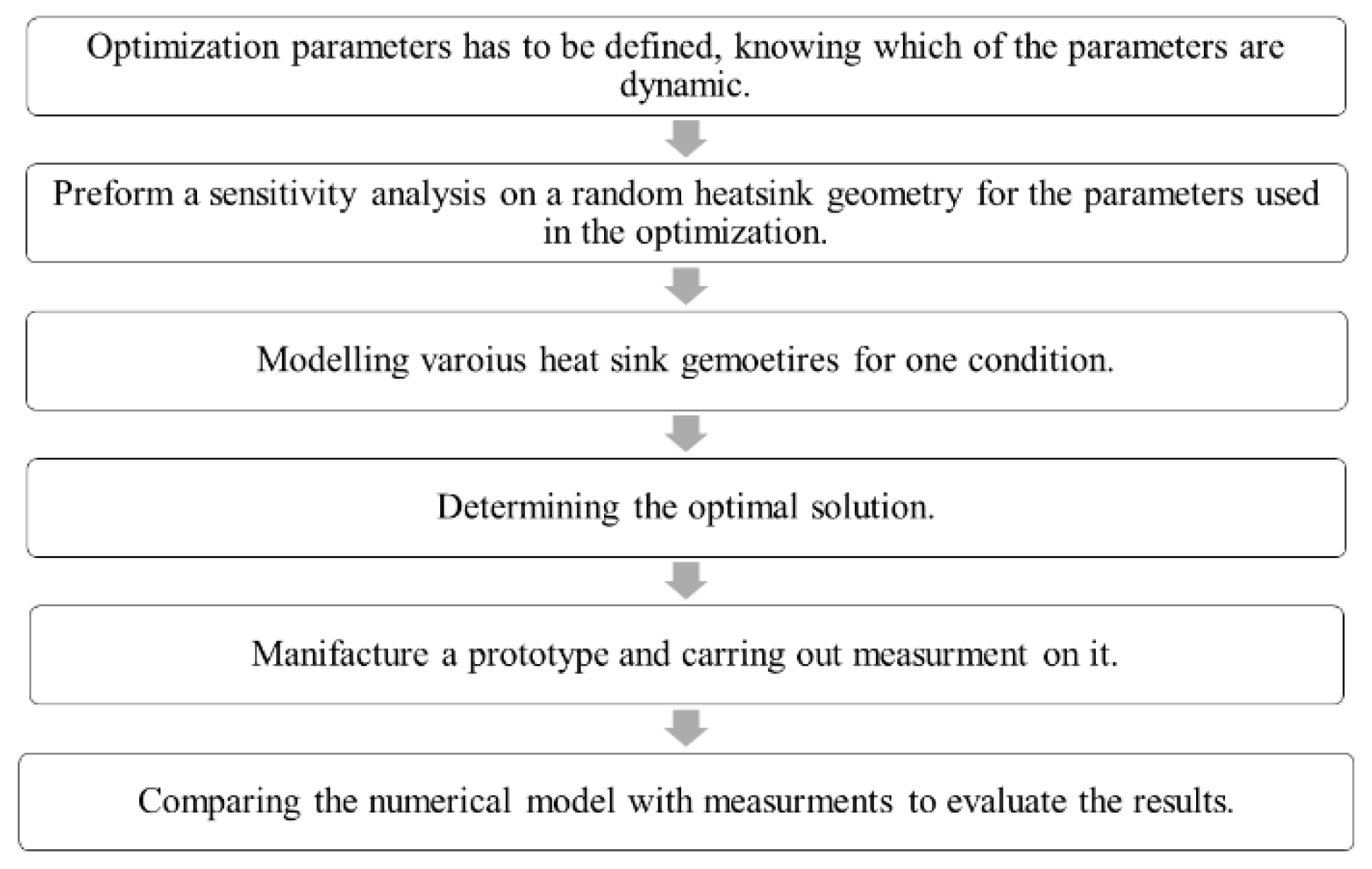
Figure 2.
Pareto diagram sketch for this study.
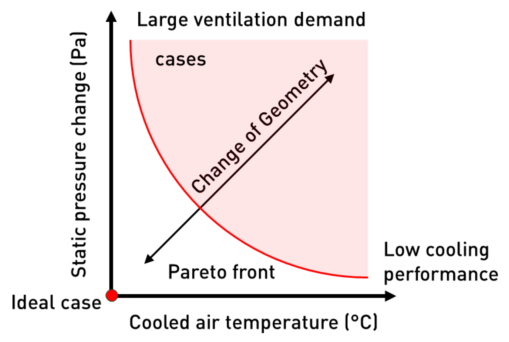
Figure 3.
Sketch of the heat sink.

Figure 4.
Sketch of the experiment.

Figure 5.
Arrangement (a) and scheme (b) of the measurement ((1) two water heat exchanger, heat sink and Peltier modules; (2) axial fan; (3) Thermometer; (4) Buffer tank; (5) Power supplies; continuous line: water pipe; dashed line: electric cable).
Figure 5.
Arrangement (a) and scheme (b) of the measurement ((1) two water heat exchanger, heat sink and Peltier modules; (2) axial fan; (3) Thermometer; (4) Buffer tank; (5) Power supplies; continuous line: water pipe; dashed line: electric cable).

Figure 6.
Sensitivity values.

Figure 7.
Boxplot of the coefficients.
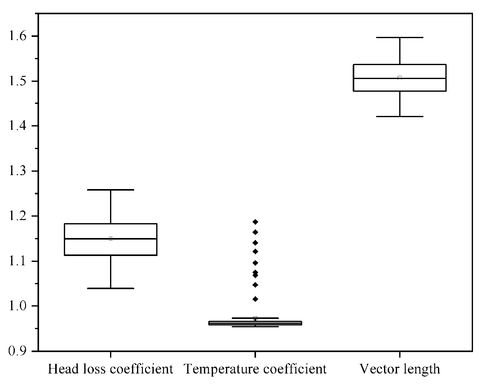
Figure 8.
Simulation results (a) all of the solution; (b) 5 most favourable solutions (with vector lengths).
Figure 8.
Simulation results (a) all of the solution; (b) 5 most favourable solutions (with vector lengths).
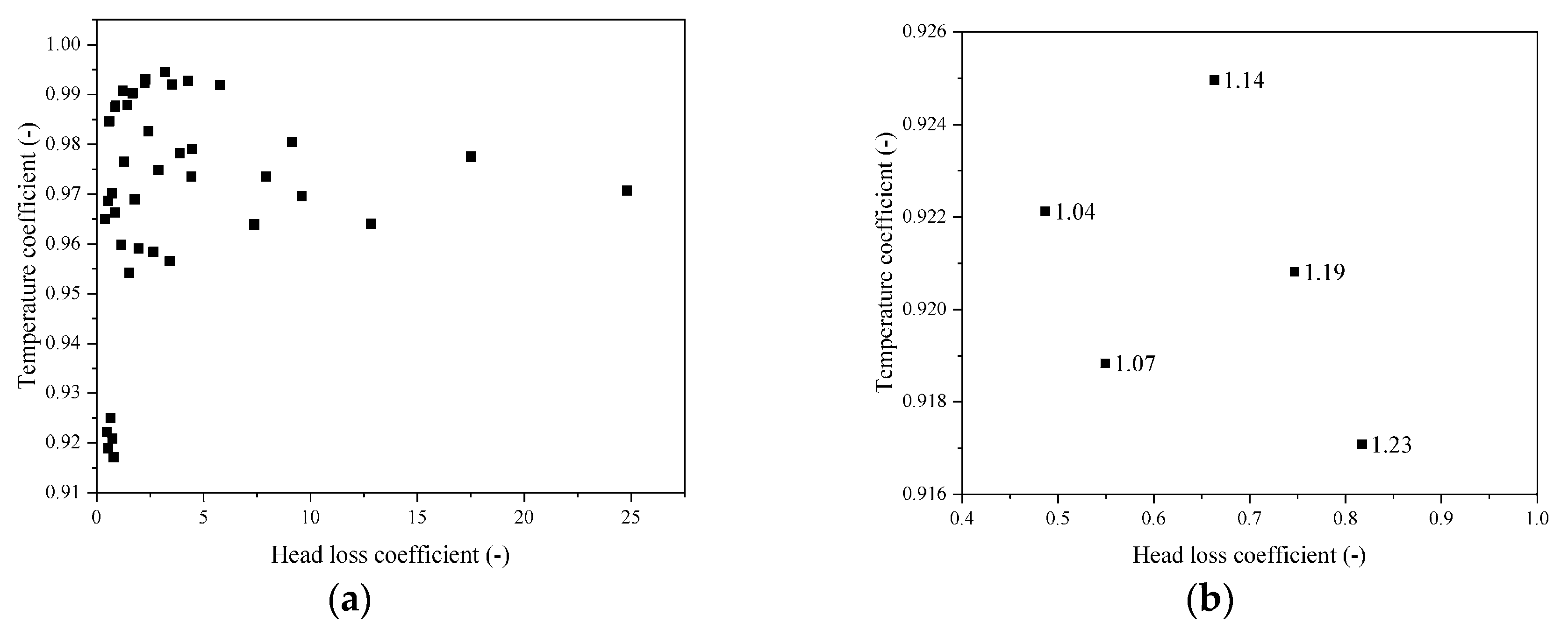
Figure 9.
Prototype heat sink (a) heat sink before the installation; (b) condensation on heat sink.


Table 1.
Conditions parameters selected for sensitivity analysis.
| Fin Number (pcs) | Fin Width (mm) | RH (%) | Tinlet (°C) | v (m s−1) | Qcold (W) |
|---|---|---|---|---|---|
| 2 | 6 | 30 | 26 | 3 | 50 |
| 50 | 32 | 4 | 100 | ||
| 70 | 38 | 5 | 150 | ||
| 200 |
Table 2.
Numerical model and solver setup.
| Module | Details |
|---|---|
| Geometry | Parametric function of fin numbers and width |
| Mesh | Cut cell method with element size of 0.5 mm and 2 pieces of 0.3 mm high inflation layers |
| Turbulence model | standard k-ε model with scalable wall functions |
| Material properties | Moist air: Section 1.2 Heat sink: (optimization) copper Heat sink: (comparison) aluminum |
| Solver | Steady state Pseudo transient method coupled velocity and pressure solver |
| Convergence criteria | Residual 10−5 |
Table 3.
Measured parameters.
| Notation | Parameter | Manufacturer | Device Type | Resolution |
|---|---|---|---|---|
| RHinlet | inlet relative humidity | KIMO | KTH-300 | 0.1% |
| RHoutlet | outlet relative humidity | KIMO | KTH-300 | 0.1% |
| Tinlet | inlet temperature | KIMO | KTH-300 | 0.1 °C |
| Toutlet | outlet temperature | KIMO | KTH-300 | 0.1 °C |
| Tcold | heat sink surface temperature | Raytek | Raynger MX4 | 1 °C |
| Δp | pressure loss | KIMO | AMI301 | 1 Pa |
| v | average air velocity | KIMO | AMI301 | 0.1 m s−1 |
| U | voltage | HESTORE | VM028-330-R | 0.1 V |
| P | power demand | REV Ritter | EMT717ACTL | 1 W |
Table 4.
Statistics of the sensitivity analysis.
| Parameters | Mean | Standard Deviation | Error |
|---|---|---|---|
| Temperature coefficient | 0.973 | ±0.042 | ±4.34% |
| Head loss coefficient | 1.15 | ±0.049 | ±4.26% |
| Vector length | 1.51 | ±0.04 | ±2.7% |
Table 5.
Cases and vector lengths.
| Fin Width (mm) | Fin Number | Vector Length |
|---|---|---|
| 6 | 1 | 1.04 |
| 2 | 2 | 1.05 |
| 7 | 1 | 1.07 |
| 3 | 2 | 1.12 |
| 8 | 1 | 1.14 |
Table 6.
Measured average values of the quasi-steady state.
| Parameter | Value | Deviation |
|---|---|---|
| RHinlet (%) | 45.15 | ±0.29 |
| RHoutlet (%) | 47.4 | ±0.26 |
| Tinlet (°C) | 17.08 | ±0.04 |
| Toutlet (°C) | 16.09 | ±0.02 |
| Tcold (°C) | −20 | - |
| U (V) | 12 | - |
| P (W) | 88 | - |
| Qcold (W) | 20 | - |
| v (m s−1) | 2.5 | ±0.2 |
| Δp (Pa) | 3 | ±1 |
Table 7.
Parameters for comparison.
| Parameter | Measured Values | Simulated | Error |
|---|---|---|---|
| Toutlet [°C] | 16.09 | 15.66 | ±3% |
| Δp [Pa] | 3 | 2.1 | ±30% |
© 2020 by the author. Licensee MDPI, Basel, Switzerland. This article is an open access article distributed under the terms and conditions of the Creative Commons Attribution (CC BY) license (http://creativecommons.org/licenses/by/4.0/).
Share and Cite
MDPI and ACS Style
Szodrai, F. Heat Sink Shape and Topology Optimization with Pareto-Vector Length Optimization for Air Cooling. Energies 2020, 13, 1661. https://doi.org/10.3390/en13071661
AMA Style
Szodrai F. Heat Sink Shape and Topology Optimization with Pareto-Vector Length Optimization for Air Cooling. Energies. 2020; 13(7):1661. https://doi.org/10.3390/en13071661
Chicago/Turabian StyleSzodrai, Ferenc. 2020. "Heat Sink Shape and Topology Optimization with Pareto-Vector Length Optimization for Air Cooling" Energies 13, no. 7: 1661. https://doi.org/10.3390/en13071661
Note that from the first issue of 2016, this journal uses article numbers instead of page numbers. See further details here.