Intelligent Road Inspection with Advanced Machine Learning; Hybrid Prediction Models for Smart Mobility and Transportation Maintenance Systems

 ,
,  , ,
, ,  , ,
, , 
Abstract
1. Introduction
2. Literature Review
- PCI prediction methods based on other pavement quality indices.
- PCI prediction methods based on pavement age.
- PCI prediction methods based on pavement surface deflection.
3. Materials and Methods
3.1. Pavement Condition Index (PCI)
- Determine the type, extent and severity of pavement distresses.
- Determine DV for each distress based on its corresponding curve [72].
- Reduce the number of DVs to the maximum number allowed by Equation (4):
- Determine the number of DVs greater than 2 (q).
- Determine total deduct value (TDV), which is the sum of DVs.
- Determine corrected deduct value (CDV) based on correction curves using q and TDV [72].
- Decrease the smallest DVs larger than 2 to 2.
- Repeat steps 4 to 7 until q reaches 1.
- Determine the maximum CDV and calculate the PCI using Equation (5):
3.2. Falling Weight Deflectometer (FWD)
3.3. Case Study
3.4. Analysis Methods
3.4.1. Multi-Layer Perceptron (MLP) Neural Network
3.4.2. Radial Basis Function (RBF) Neural Network
3.4.3. Committee Machine Intelligent System (CMIS)
3.5. Performance Criteria
4. Results and Discussion
5. Conclusions
Author Contributions
Funding
Acknowledgments
Conflicts of Interest
Abbreviations
| Abbreviation | Description |
| PCI | Pavement Condition Index |
| FWD | Falling Weight Deflectometer |
| MLP | Multi-layer perceptron |
| RBF | Radial Basis Function |
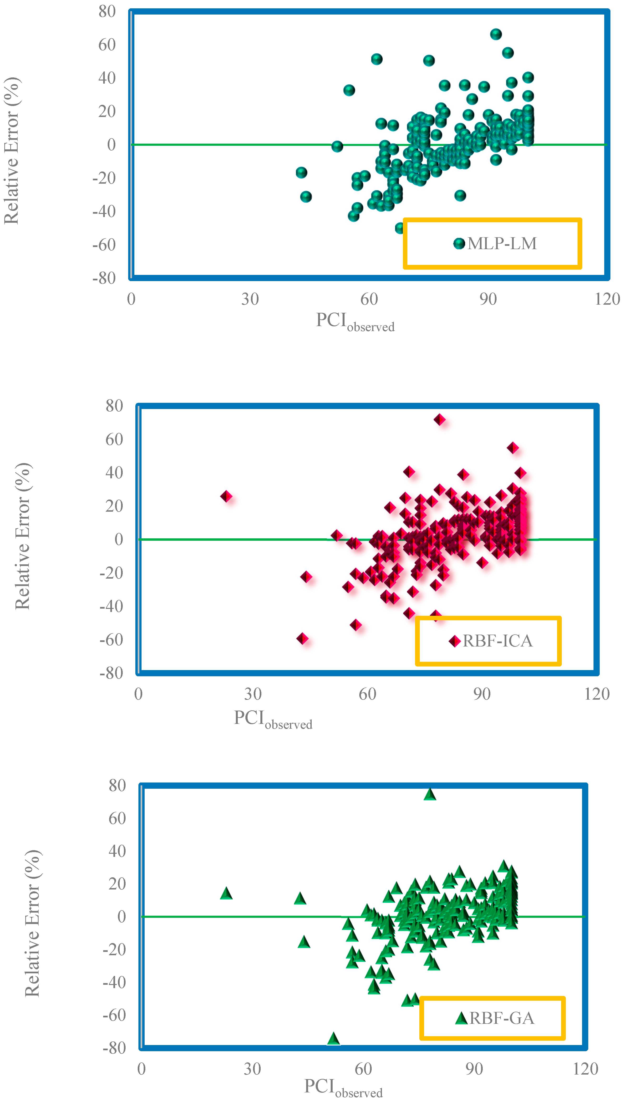
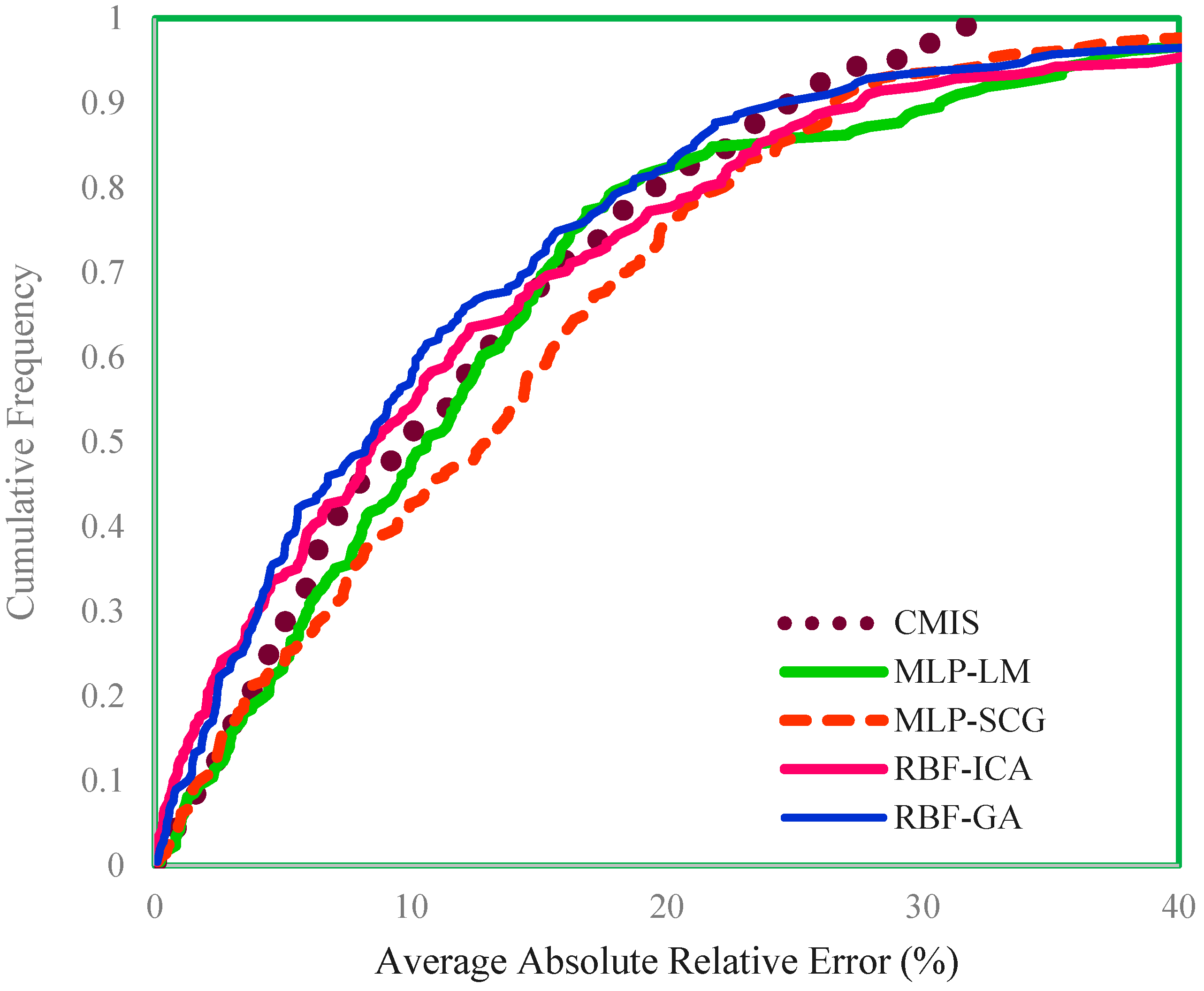
| MLP-LM | Multi-layer perceptron Optimized by Levenberg-Marquardt Algorithm |
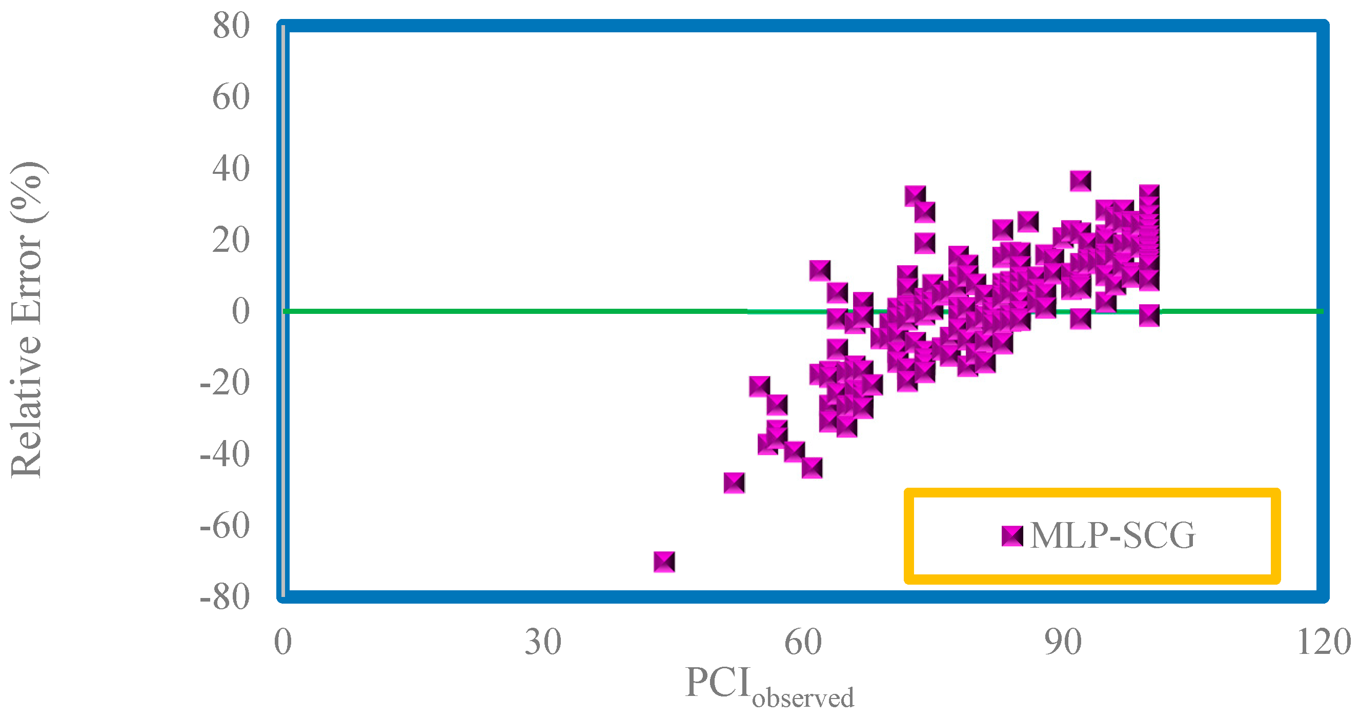
| MLP-SCG | Multi-layer perceptron Optimized by Scaled Conjugate Gradient Algorithm |
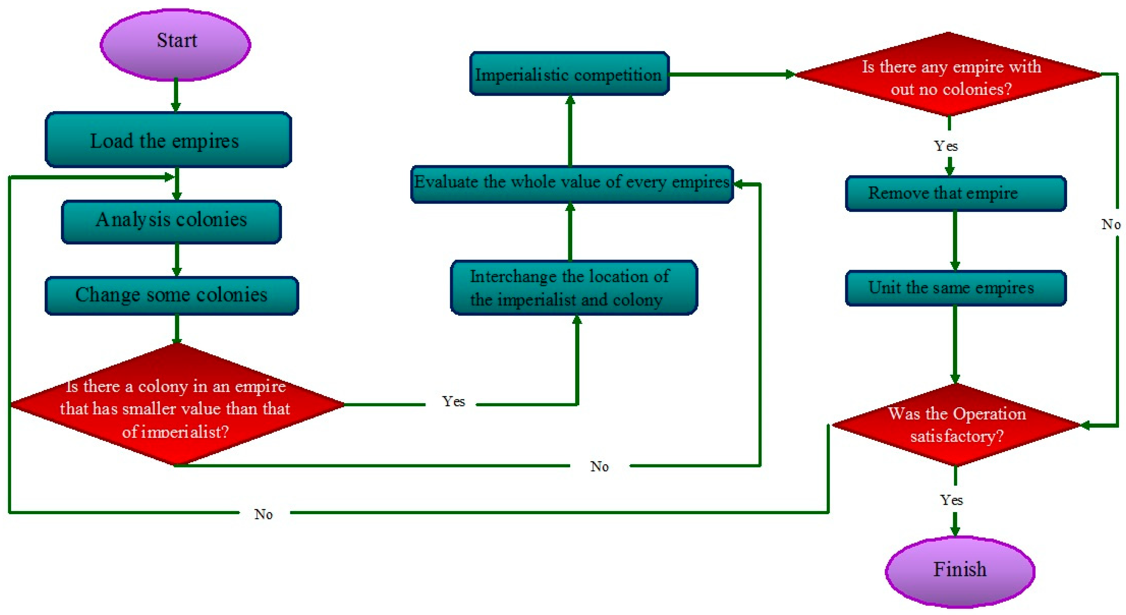
| RBF-ICA | Radial Basis Function Optimized by Imperialist Competitive Algorithm |
| RBF-GA | Radial Basis Function Optimized by Genetic Algorithm |
| CMIS | Committee Machine Intelligent Systems |
| APRE | Average Percent Relative Error |
| AAPRE | Average Absolute Percent Relative Error |
| RMSE | Root Mean Square Error |
| SE | Standard Error |
| MR&R | Maintenance, Rehabilitation, and Reconstruction |
| PMS | Pavement Management System |
| GPR | Ground Penetrating Radar |
| LS | Laser System |
| ANN | Artificial Neural Network |
| SVM | Support Vector Machine |
| RF | Random Forest |
| DL | Deep Learning |
| DM | Data Mining |
| GMDH | Group Method of Data Handling |
| GEP | Gene Expression Programming |
| ANN/SA | Artificial Neural Network/Simulated Annealing |
| ML | Machine Learning |
| DV | Deduct Value |
| TDV | Total Deduct Value |
| CDV | Corrected Deduct Value |
| CG | Conjugate Gradient |
| RWD | Rolling Weight Deflectometer |
| TSD | Traffic Speed Deflectometer |
References
- France-Mensah, J.; O’Brien, W.J. Developing a Sustainable Pavement Management Plan: Tradeoffs in Road Condition, User Costs, and Greenhouse Gas Emissions. J. Manag. Eng. 2019, 35, 4019005. [Google Scholar] [CrossRef]
- Suraji, A.; Sudjianto, A.T.; Riman, R. Analysis of Road Surface Defects Using Road Condition Index Method on the Caruban-Ngawi Road Segment. J. Sci. Appl. Eng. 2018, 1, 1. [Google Scholar] [CrossRef]
- Elbagalati, O.; Elseifi, M.A.; Gaspard, K.; Zhang, Z. Prediction of In-Service Pavement Structural Capacity Based on Traffic-Speed Deflection Measurements. J. Transp. Eng. 2016, 142, 4016058. [Google Scholar] [CrossRef]
- Shrestha, S.; Katicha, S.W.; Flintsch, G.W. Pavement Condition Data from Traffic Speed Deflectometer for Network Level Pavement Management. In Airfield and Highway Pavements 2019; American Society of Civil Engineers (ASCE): Reston, VA, USA, 2019; pp. 392–403. [Google Scholar]
- Mack, J.W.; Sullivan, R.L. Using remaining service life as the national performance measure of pavement assets 2. In Proceedings of the Annual Meeting of the Transportation Research Board, Washington, DC, USA, 13–17 January 2013; p. 32. [Google Scholar]
- Kuo, C.-M.; Tsai, T.-Y. Significance of subgrade damping on structural evaluation of pavements. Road Mater. Pavement Des. 2014, 15, 455–464. [Google Scholar] [CrossRef]
- Bryce, J.; Flintsch, G.; Katicha, S.; Diefenderfer, B. Enhancing Network-Level Decision Making through the use of a Structural Capacity Index. Transp. Res. Rec. J. Transp. Res. Board 2013, 2366, 64–70. [Google Scholar] [CrossRef]
- Loprencipe, G.; Pantuso, A.; Di Mascio, P. Sustainable Pavement Management System in Urban Areas Considering the Vehicle Operating Costs. Sustainability 2017, 9, 453. [Google Scholar] [CrossRef]
- Shah, Y.U.; Jain, S.; Tiwari, D.; Jain, M. Development of Overall Pavement Condition Index for Urban Road Network. Procedia Soc. Behav. Sci. 2013, 104, 332–341. [Google Scholar] [CrossRef]
- Kumlai, A.; Sangpetngam, B.; Chalempong, S. Development of equations for determining layer elastic moduli using pavement deflection characteristics. TRB Pap. 2013, 92, 14–0976. [Google Scholar]
- Long, B.; Shatnawi, S. Structural evaluation of rigid pavement sections. Road Mater. Pavement Des. 2000, 1, 97–117. [Google Scholar] [CrossRef]
- García, J.A.R.; Castro, M. Analysis of the temperature influence on flexible pavement deflection. Constr. Build. Mater. 2011, 25, 3530–3539. [Google Scholar] [CrossRef]
- Djaha, S.I.K.; Prayuda, H. Quality Assessment of Road Pavement using Lightweight Deflectometer. In Proceedings of the Third International Conference on Sustainable Innovation 2019—Technology and Engineering (IcoSITE 2019), Yogyakarta, Indonesia, 30–31 July 2019; Atlantis Press: Paris, France, 2019. [Google Scholar]
- Ullidtz, P. Pavement Analysis. Developments in Civil Engineering; North Holland: Amsterdam, The Netherlands, 1987. [Google Scholar]
- Kutay, M.E.; Chatti, K.; Lei, L. Backcalculation of Dynamic Modulus Mastercurve from Falling Weight Deflectometer Surface Deflections. Transp. Res. Rec. J. Transp. Res. Board 2011, 2227, 87–96. [Google Scholar] [CrossRef]
- Karballaeezadeh, N.; Mohammadzadeh, S.D.; Shamshirband, S.; Hajikhodaverdikhan, P.; Mosavi, A.; Chau, K.-W. Prediction of remaining service life of pavement using an optimized support vector machine (case study of Semnan–Firuzkuh road). Eng. Appl. Comput. Fluid Mech. 2019, 13, 188–198. [Google Scholar] [CrossRef]
- Kargah-Ostadi, N. Comparison of Machine Learning Techniques for Developing Performance Prediction Models. In Computing in Civil and Building Engineering (2014); American Society of Civil Engineers: Reston, VA, USA, 2014; pp. 1222–1229. [Google Scholar]
- Chou, J.; O’Neill, W.; Cheng, H. Pavement distress classification using neural networks. In Proceedings of the IEEE International Conference on Systems, Man and Cybernetics, San Antonio, TX, USA, 3–5 October 2002; Volume 1, pp. 397–401. [Google Scholar]
- Eldin, N.N.; Senouci, A. Condition rating of rigid pavements by neural networks. Can. J. Civ. Eng. 1995, 22, 861–870. [Google Scholar] [CrossRef]
- Owusu-Ababio, S. Application of Neural Networks to Modeling Thick Asphalt Pavement Performance. Artif. Intell. Math. Methods Pavement Geomech. Syst. 1998, 25, 23–30. [Google Scholar]
- Sundin, S.; Braban-Ledoux, C. Artificial Intelligence–Based Decision Support Technologies in Pavement Management. Comput. Civ. Infrastruct. Eng. 2001, 16, 143–157. [Google Scholar] [CrossRef]
- Yang, J.; Lu, J.J.; Gunaratne, M.; Xiang, Q. Forecasting Overall Pavement Condition with Neural Networks: Application on Florida Highway Network. Transp. Res. Rec. J. Transp. Res. Board 2003, 1853, 3–12. [Google Scholar] [CrossRef]
- Gopalakrishnan, K. Neural Network–Swarm Intelligence Hybrid Nonlinear Optimization Algorithm for Pavement Moduli Back-Calculation. J. Transp. Eng. 2010, 136, 528–536. [Google Scholar] [CrossRef]
- Terzi, S.; Saltan, M.; Küçüksille, E.U.; Karaşahin, M. Backcalculation of pavement layer thickness using data mining. Neural Comput. Appl. 2012, 23, 1369–1379. [Google Scholar] [CrossRef]
- Nejad, F.M.; Motekhases, F.Z.; Zakeri, H.; Wang, L.-J.; Monaghan, J.M. An Image Processing Approach to Asphalt Concrete Feature Extraction. J. Ind. Intell. Inf. 2014, 3, 3. [Google Scholar] [CrossRef]
- Ziari, H.; Maghrebi, M.; Ayoubinejad, J.; Waller, T. Prediction of Pavement Performance: Application of Support Vector Regression with Different Kernels. Transp. Res. Rec. J. Transp. Res. Board 2016, 2589, 135–145. [Google Scholar] [CrossRef]
- Georgiou, P.; Plati, C.; Loizos, A. Soft Computing Models to Predict Pavement Roughness: A Comparative Study. Adv. Civ. Eng. 2018, 2018, 1–8. [Google Scholar] [CrossRef]
- Fathi, A.; Mazari, M.; Saghafi, M.; Hosseini, A.; Kumar, S. Parametric Study of Pavement Deterioration Using Machine Learning Algorithms. In Airfield and Highway Pavements 2019; American Society of Civil Engineers (ASCE): Reston, VA, USA, 2019; pp. 31–41. [Google Scholar]
- Santos, J.; Ferreira, A.; Flintsch, G. An adaptive hybrid genetic algorithm for pavement management. Int. J. Pavement Eng. 2017, 20, 266–286. [Google Scholar] [CrossRef]
- Zakeri, H.; Nejad, F.M.; Fahimifar, A. Image Based Techniques for Crack Detection, Classification and Quantification in Asphalt Pavement: A Review. Arch. Comput. Methods Eng. 2016, 24, 935–977. [Google Scholar] [CrossRef]
- Cheng, H.; Miyojim, M. Automatic pavement distress detection system. Inf. Sci. 1998, 108, 219–240. [Google Scholar] [CrossRef]
- Huang, J.; Liu, W.; Sun, X. A Pavement Crack Detection Method Combining 2D with 3D Information Based on Dempster-Shafer Theory. Comput. Civ. Infrastruct. Eng. 2013, 29, 299–313. [Google Scholar] [CrossRef]
- Inzerillo, L.; Di Mino, G.; Roberts, R. Image-based 3D reconstruction using traditional and UAV datasets for analysis of road pavement distress. Autom. Constr. 2018, 96, 457–469. [Google Scholar] [CrossRef]
- Chen, D.; Sefidmazgi, N.R.; Bahia, H. Exploring the feasibility of evaluating asphalt pavement surface macro-texture using image-based texture analysis method. Road Mater. Pavement Des. 2015, 16, 405–420. [Google Scholar] [CrossRef]
- Wu, L.; Mokhtari, S.; Nazef, A.; Nam, B.; Yun, H.-B. Improvement of Crack-Detection Accuracy Using a Novel Crack Defragmentation Technique in Image-Based Road Assessment. J. Comput. Civ. Eng. 2016, 30, 04014118. [Google Scholar] [CrossRef]
- Han, J.-Y.; Chen, A.; Lin, Y.-T. Image-Based Approach for Road Profile Analyses. J. Surv. Eng. 2016, 142, 06015003. [Google Scholar] [CrossRef]
- Solla, M.; Lagüela, S.; González-Jorge, H.; Arias, P. Approach to identify cracking in asphalt pavement using GPR and infrared thermographic methods: Preliminary findings. NDT E Int. 2014, 62, 55–65. [Google Scholar] [CrossRef]
- Chapeleau, X.; Blanc, J.; Hornych, P.; Gautier, J.-L.; Carroget, J. Use of distributed fiber optic sensors to detect damage in a pavement. Asph. Pavements 2014, 449–457. [Google Scholar]
- Chang, K.-T.; Chang, J.-R.; Liu, J.-K. Detection of Pavement Distresses Using 3D Laser Scanning Technology. In Computing in Civil Engineering (2005); American Society of Civil Engineers (ASCE): Reston, VA, USA, 2005; pp. 1–11. [Google Scholar]
- Bitelli, G.; Simone, A.; Girardi, F.; Lantieri, C. Laser Scanning on Road Pavements: A New Approach for Characterizing Surface Texture. Sensors 2012, 12, 9110–9128. [Google Scholar] [CrossRef] [PubMed]
- Tsai, Y.-C.; Li, F. Critical Assessment of Detecting Asphalt Pavement Cracks under Different Lighting and Low Intensity Contrast Conditions Using Emerging 3D Laser Technology. J. Transp. Eng. 2012, 138, 649–656. [Google Scholar] [CrossRef]
- Park, K.; Thomas, N.; Lee, K.W. Applicability of the International Roughness Index as a Predictor of Asphalt Pavement Condition1. J. Transp. Eng. 2007, 133, 706–709. [Google Scholar] [CrossRef]
- Dewan, S.; Smith, R. Estimating IRI from pavement distresses to calculate vehicle operating costs for the cities and counties of San Francisco Bay area. Transp. Res. Rec. J. Transp. Res. Board 2002, 1816, 65–72. [Google Scholar] [CrossRef]
- Arhin, S.A.; Williams, L.N.; Ribbiso, A.; Anderson, M.F. Predicting pavement condition index using international roughness index in a dense urban area. J. Civil. Eng. Res. 2015, 5, 10–17. [Google Scholar]
- Suh, Y.-C.; Kwon, H.-J.; Park, K.-S.; Ohm, B.-S.; Kim, B.-I. Correlation Analysis between Pavement Condition Indices in Korean Roads. KSCE J. Civ. Eng. 2017, 22, 1162–1169. [Google Scholar] [CrossRef]
- Ningyuan, L.; Kazmierowski, T.; Tighe, S.; Haas, R. Integrating dynamic performance prediction models into pavement management maintenance and rehabilitation programs. In Proceedings of the 5th International Conference on Managing Pavements, Chicago, IL, USA, 11–14 August 2001. [Google Scholar]
- Khattak, M.J. Development of Uniform Sections for PMS Inventory and Application-Interim Report; Louisiana Transportation Research Center: Baton Rouge, LA, USA, 2009.
- Chen, J.-S.; Wangdi, K. Proposal of a New Road Surface Management System(RSMS) for Developing Countries. Doboku Gakkai Ronbunshu 1999, 618, 83–94. [Google Scholar] [CrossRef]
- Yuan, J.; Mooney, M.A. Development of Adaptive Performance Models for Oklahoma Airfield Pavement Management System. Transp. Res. Rec. J. Transp. Res. Board 2003, 1853, 44–54. [Google Scholar] [CrossRef]
- Michels, D.J. Pavement Condition Index and Cost of Ownership Analysis on Preventative Maintenance Projects in Kentucky. Master’s Thesis, University of Kentucky, Lexington, KY, USA, 2017. [Google Scholar]
- O’Brien, D.E., III; Kohn, S.D.; Shahin, M.Y. Prediction of Pavement Performance by Using Nondestructive Test Results. Transp. Res. Rec. 1983, 943, 13. [Google Scholar]
- Nivedya, M.; Mallick, R.B. Accurate prediction of laboratory permeability of hot mix asphalt using machine learning techniques. In Proceedings of the Advances in Materials and Pavement Performance Prediction, Doha, Qatar, 16–18 April 2018; pp. 133–137. [Google Scholar]
- Nivedya, M.K.; Mallick, R.B. A multi-structure multi-run range (MSMRR) approach for using machine learning with constrained data in pavement engineering. SN Appl. Sci. 2020, 2, 1–10. [Google Scholar] [CrossRef]
- Inkoom, S.; Sobanjo, J.; Barbu, A.; Niu, X. Prediction of the crack condition of highway pavements using machine learning models. Struct. Infrastruct. Eng. 2019, 15, 940–953. [Google Scholar] [CrossRef]
- Lin, J.-D.; Yau, J.-T.; Hsiao, L.-H. Correlation analysis between international roughness index (IRI) and pavement distress by neural network. In Proceedings of the 82nd Annual Meeting of the Transportation Research Board, Washington, DC, USA, 12–16 January 2003; pp. 12–16. [Google Scholar]
- Bianchini, A.; Bandini, P. Prediction of Pavement Performance through Neuro-Fuzzy Reasoning. Comput. Civ. Infrastruct. Eng. 2010, 25, 39–54. [Google Scholar] [CrossRef]
- Kargah-Ostadi, N.; Stoffels, S.M.; Tabatabaee, N. Network-Level Pavement Roughness Prediction Model for Rehabilitation Recommendations. Transp. Res. Rec. J. Transp. Res. Board 2010, 2155, 124–133. [Google Scholar] [CrossRef]
- Kargah-Ostadi, N.; Stoffels, S.M. Framework for Development and Comprehensive Comparison of Empirical Pavement Performance Models. J. Transp. Eng. 2015, 141, 4015012. [Google Scholar] [CrossRef]
- Ziari, H.; Sobhani, J.; Ayoubinejad, J.; Hartmann, T. Prediction of IRI in short and long terms for flexible pavements: ANN and GMDH methods. Int. J. Pavement Eng. 2015, 17, 1–13. [Google Scholar] [CrossRef]
- Hoang, N.-D.; Nguyen, Q.-L. A novel method for asphalt pavement crack classification based on image processing and machine learning. Eng. Comput. 2018, 35, 487–498. [Google Scholar] [CrossRef]
- Mazari, M.; Rodriguez, D.D. Prediction of pavement roughness using a hybrid gene expression programming-neural network technique. J. Traffic Transp. Eng. (English Ed.) 2016, 3, 448–455. [Google Scholar] [CrossRef]
- Nabipour, N.; Karballaeezadeh, N.; Dineva, A.; Mosavi, A.; Mohammadzadeh, S.D.; Shamshirband, S. Comparative Analysis of Machine Learning Models for Prediction of Remaining Service Life of Flexible Pavement. Mathematics 2019, 7, 1198. [Google Scholar] [CrossRef]
- Fujita, Y.; Shimada, K.; Ichihara, M.; Hamamoto, Y. A method based on machine learning using hand-crafted features for crack detection from asphalt pavement surface images. In Proceedings of the Thirteenth International Conference on Quality Control by Artificial Vision 2017, Tokyo, Japan, 14–16 May 2017; Volume 10338, p. 103380. [Google Scholar]
- Marcelino, P.; Antunes, M.D.L.; Fortunato, E.; Gomes, M.C. Machine learning approach for pavement performance prediction. Int. J. Pavement Eng. 2019, 1–14. [Google Scholar] [CrossRef]
- Zhang, A.; Wang, K.C.P.; Li, B.; Yang, E.; Dai, X.; Peng, Y.; Fei, Y.; Liu, Y.; Li, J.Q.; Chen, C. Automated Pixel-Level Pavement Crack Detection on 3D Asphalt Surfaces Using a Deep-Learning Network. Comput. Civ. Infrastruct. Eng. 2017, 32, 805–819. [Google Scholar] [CrossRef]
- Ziari, H.; Sobhani, J.; Ayoubinejad, J.; Hartmann, T. Analysing the accuracy of pavement performance models in the short and long terms: GMDH and ANFIS methods. Road Mater. Pavement Des. 2015, 17, 1–19. [Google Scholar] [CrossRef]
- Majidifard, H.; Jahangiri, B.; Buttlar, W.G.; Alavi, A.H. New machine learning-based prediction models for fracture energy of asphalt mixtures. Measurement 2019, 135, 438–451. [Google Scholar] [CrossRef]
- Marcelino, P.; Antunes, M.D.L.; Fortunato, E.; Gomes, M.C. Machine Learning for Pavement Friction Prediction Using Scikit-Learn. In Proceedings of the Requirements Engineering: Foundation for Software Quality, Essen, Germany, 27 February–2 March 2017; Volume 10423, pp. 331–342. [Google Scholar]
- Shahin, M.Y.; Kohn, S.D. Pavement Maintenance Management for Roads and Parking Lots; Construction Engineering Research Lab (Army): Champaign, IL, USA, 1981. [Google Scholar]
- Shahnazari, H.; Tutunchian, M.A.; Mashayekhi, M.; Amini, A.A. Application of Soft Computing for Prediction of Pavement Condition Index. J. Transp. Eng. 2012, 138, 1495–1506. [Google Scholar] [CrossRef]
- ASTM D6433-07. Standard Practice for Roads and Parking Lots Pavement Condition Index Surveys; American Society for Testing and Materials: West Conshohocken, PA, USA, 2007. [Google Scholar]
- Shahin, M.Y. Pavement Management for Airports, Roads, and Parking Lots; Springer: Berlin/Heidelberg, Germany, 1994; Volume 501. [Google Scholar]
- Levenberg, E.; Pettinari, M.; Baltzer, S.; Christensen, B.M.L. Comparing Traffic Speed Deflectometer and Falling Weight Deflectometer Data. Transp. Res. Rec. J. Transp. Res. Board 2018, 2672, 22–31. [Google Scholar] [CrossRef]
- Nejad, F.M.; Mehrabi, A.; Zakeri, H. Prediction of Asphalt Mixture Resistance Using Neural Network via Laboratorial X-ray Images. J. Ind. Intell. Inf. 2014, 3, 3. [Google Scholar] [CrossRef]
- Yu, H.; Wilamowski, B. Levenberg–Marquardt Training. VLSI Handb. 2011, 5, 1–16. [Google Scholar]
- Huang, C.; Chen, F.; Chang, Y.; Han, L.; Li, S.; Hong, J. Adaptive Operator-Based Spectral Deconvolution with the Levenberg-Marquardt Algorithm. Photon. Sens. 2019, 11, 1–12. [Google Scholar] [CrossRef]
- Hagan, M.; Menhaj, M. Training feedforward networks with the Marquardt algorithm. IEEE Trans. Neural Netw. 1994, 5, 989–993. [Google Scholar] [CrossRef]
- Møller, M.F. A scaled conjugate gradient algorithm for fast supervised learning. Neural Netw. 1993, 6, 525–533. [Google Scholar] [CrossRef]
- Kişi, Ö.; Uncuoğlu, E. Comparison of Three Back-Propagation Training Algorithms for Two Case Studies; CSIR: Pretoria, South Africa, 2005. [Google Scholar]
- Broomhead, D.S.; Lowe, D. Radial Basis Functions, Multi-Variable Functional Interpolation and Adaptive Networks; Royal Signals and Radar Establishment Malvern: Malvern, UK, 1988. [Google Scholar]
- Sheng, Z. Pavement performance evaluating model by using RBF. J. Highw. Transp. Res. Dev. 2008, 3, 23–26. [Google Scholar]
- Yildirim, S.; Uzmay, I. Statistical analysis of vehicles’ vibration due to road roughness using radial basis artificial neural network. Appl. Artif. Intell. 2001, 15, 419–427. [Google Scholar] [CrossRef]
- Karim, A.; Adeli, H. Radial Basis Function Neural Network for Work Zone Capacity and Queue Estimation. J. Transp. Eng. 2003, 129, 494–503. [Google Scholar] [CrossRef]
- Ardabili, S.F.; Mahmoudi, A.; Gundoshmian, T.M. Modeling and simulation controlling system of HVAC using fuzzy and predictive (radial basis function, RBF) controllers. J. Build. Eng. 2016, 6, 301–308. [Google Scholar] [CrossRef]
- Davis, L. Handbook of Genetic Algorithms; Van Nostrand Reinhold: New York, NY, USA, 1991. [Google Scholar]
- Alam, N.; Das, B.; Pant, V. A comparative study of metaheuristic optimization approaches for directional overcurrent relays coordination. Electr. Power Syst. Res. 2015, 128, 39–52. [Google Scholar] [CrossRef]
- Atashpaz-Gargari, E.; Lucas, C. Imperialist competitive algorithm: An algorithm for optimization inspired by imperialistic competition. In Proceedings of the 2007 IEEE Congress on Evolutionary Computation, Singapore, 25–28 September 2007; pp. 4661–4667. [Google Scholar]
- Hosseini, S.; Al Khaled, A. A survey on the Imperialist Competitive Algorithm metaheuristic: Implementation in engineering domain and directions for future research. Appl. Soft Comput. 2014, 24, 1078–1094. [Google Scholar] [CrossRef]
- Nilsson, N.J. Learning Machines; American Psychological Association: Washington, DC, USA, 1965. [Google Scholar]
- Hashem, S.; Schmeiser, B. Approximating a Function and Its Derivatives Using MSE-Optimal Linear Combinations of Trained Feedforward Neural Networks; Purdue University, Department of Statistics: West Lafayette, IN, USA, 1993. [Google Scholar]
- Perrone, M.P.; Cooper, L.N. When networks disagree: Ensemble methods for hybrid neural networks; Brown Univ Providence Ri Inst for Brain and Neural Systems: Providence, RI, USA, 1992. [Google Scholar]
- Sarapardeh, A.H.; Varamesh, A.; Husein, M.M.; Karan, K. On the evaluation of the viscosity of nanofluid systems: Modeling and data assessment. Renew. Sustain. Energy Rev. 2018, 81, 313–329. [Google Scholar] [CrossRef]
- Ardabili, S.F.; Najafi, B.; Alizamir, M.; Mosavi, A.; Shamshirband, S.; Rabczuk, T. Using SVM-RSM and ELM-RSM Approaches for Optimizing the Production Process of Methyl and Ethyl Esters. Energies 2018, 11, 2889. [Google Scholar] [CrossRef]


| Damage (%) | Condition | Maintenance Program |
|---|---|---|
| <6 | Good | Routine Maintenance |
| 6–11 | Moderate | Minor Rehabilitation |
| 11–15 | Light Damage | Major Rehabilitation |
| >15 | Heavy Damage | Reconstruction |
| Model | Equation | Description |
|---|---|---|
| Park et al. [42] | IRI: International roughness index. | |
| Dewan and Smith [43] | IRI: International roughness index. | |
| Arhin et al. [44] | IRI: International roughness index, A and K: Regression coefficients, : Error | |
| Korea institute of construction technology [45] | NHPCI: National highway pavement condition index, xRD: Ruth depth (mm), xCR: Crack ration (%), xIRI: International roughness index (m/km). | |
| Korea expressway corporation research institute [45] | HPCI: Highway pavement condition index, RD: Ruth depth (mm), IRI: International roughness index (m/km), SD: Surface distress (crack quantity converted to area) (m2). | |
| Ningyuan et al. [46] | DMI: Distress manifestation index, Ci: Calibration coefficient for pavement type, RCI: Riding comfort index. | |
| Khattak et al. [47] | RNDM: Random cracking index, ALCR: Alligator cracking index, PTCH: Patch index, RUFF: Roughness index, RUT: Rutting index. |
| Model | Equation | Description |
|---|---|---|
| South Dakota Department of Transportation [48] | a: Maximum value of PCI, Age: Age of pavement (year), b: Slop coefficient of performance curve, c: Power coefficient for performance curve. | |
| Oklahoma airfield pavement management system [49] | ai: Polynomial parameters, x: Pavement age, n: Polynomial order. | |
| Michles [50] | Treatment type: 0 for microsurfacing and 1 for thin overlay, Age: Pavement age (year). |
| PCI | 0–10 | 10–25 | 25–40 | 40–55 | 55–70 | 70–85 | 85–100 |
| Condition | Failed | Serious | Very poor | Poor | Fair | Satisfactory | Good |
| No. of Coefficients | Coefficients |
|---|---|
| C1 | 0 |
| C2 | 0.657295 |
| C3 | 0.227583 |
| C4 | 0.069749 |
| C5 | 0.04656 |
| Model | Data | APRE (%) | AAPRE (%) | RMSE | SE |
|---|---|---|---|---|---|
| CMIS | Train | 3.5636 | 11.6098 | 12.0543 | 0.020082 |
| Test | −2.632 | 11.9464 | 11.807884 | 0.025687 | |
| Total | 2.3303 | 11.6768 | 12.005653 | 0.021081 | |
| MLP-LM | Train | −1.2093 | 14.9275 | 14.541231 | 0.078995 |
| Test | 4.7599 | 12.7179 | 14.330003 | 0.027158 | |
| Total | −0.02115 | 14.4877 | 14.499431 | 0.068174 | |
| MLP-SCG | Train | −0.1949 | 15.5046 | 14.167214 | 0.070149 |
| Test | 6.6833 | 13.5662 | 15.145498 | 0.031747 | |
| Total | 1.1742 | 15.1187 | 14.367255 | 0.062318 | |
| RBF-GA | Train | −0.4446 | 11.8509 | 13.003455 | 0.032987 |
| Test | 14.2997 | 19.406 | 58.919147 | 0.360989 | |
| Total | 2.4902 | 13.3547 | 28.747779 | 0.096868 | |
| RBF-ICA | Train | −0.5063 | 12.6392 | 17.077364 | 0.057202 |
| Test | 16.7628 | 25.886 | 45.214386 | 0.45286 | |
| Total | 2.9311 | 15.276 | 25.308415 | 0.134177 |
© 2020 by the authors. Licensee MDPI, Basel, Switzerland. This article is an open access article distributed under the terms and conditions of the Creative Commons Attribution (CC BY) license (http://creativecommons.org/licenses/by/4.0/).
Share and Cite
Karballaeezadeh, N.; Zaremotekhases, F.; Shamshirband, S.; Mosavi, A.; Nabipour, N.; Csiba, P.; Várkonyi-Kóczy, A.R. Intelligent Road Inspection with Advanced Machine Learning; Hybrid Prediction Models for Smart Mobility and Transportation Maintenance Systems. Energies 2020, 13, 1718. https://doi.org/10.3390/en13071718
Karballaeezadeh N, Zaremotekhases F, Shamshirband S, Mosavi A, Nabipour N, Csiba P, Várkonyi-Kóczy AR. Intelligent Road Inspection with Advanced Machine Learning; Hybrid Prediction Models for Smart Mobility and Transportation Maintenance Systems. Energies. 2020; 13(7):1718. https://doi.org/10.3390/en13071718
Chicago/Turabian StyleKarballaeezadeh, Nader, Farah Zaremotekhases, Shahaboddin Shamshirband, Amir Mosavi, Narjes Nabipour, Peter Csiba, and Annamária R. Várkonyi-Kóczy. 2020. "Intelligent Road Inspection with Advanced Machine Learning; Hybrid Prediction Models for Smart Mobility and Transportation Maintenance Systems" Energies 13, no. 7: 1718. https://doi.org/10.3390/en13071718
APA StyleKarballaeezadeh, N., Zaremotekhases, F., Shamshirband, S., Mosavi, A., Nabipour, N., Csiba, P., & Várkonyi-Kóczy, A. R. (2020). Intelligent Road Inspection with Advanced Machine Learning; Hybrid Prediction Models for Smart Mobility and Transportation Maintenance Systems. Energies, 13(7), 1718. https://doi.org/10.3390/en13071718