
A Data Driven RUL Estimation Framework of Electric Motor Using Deep Electrical Feature Learning from Current Harmonics and Apparent Power


1
Department of Mechanical Engineering (Department of Aeronautics, Mechanical and Electronic Convergence Engineering), Kumoh National Institute of Technology, Gumi 39177, Korea
2
Department of Mechanical System Engineering, Kumoh National Institute of Technology, Gumi 39177, Korea
*
Author to whom correspondence should be addressed.
Energies 2021, 14(11), 3156; https://doi.org/10.3390/en14113156
Submission received: 3 May 2021
/
Revised: 23 May 2021
/
Accepted: 26 May 2021
/
Published: 28 May 2021
(This article belongs to the Special Issue Data-Protection Combined with Machine Learning for AI-Integrated Smart Power Systems)
Abstract
:An effective remaining useful life (RUL) estimation method is of great concern in industrial machinery to ensure system reliability and reduce the risk of unexpected failures. Anticipation of an electric motor’s future state can improve the yield of a system and warrant the reuse of the industrial asset. In this paper, we present an effective RUL estimation framework of brushless DC (BLDC) motor using third harmonic analysis and output apparent power monitoring. In this work, the mechanical output of the BLDC motor is monitored through a coupled generator. To emphasize the total power generation, we have analyzed the trend of apparent power, which preserves the characteristics of real power and reactive power in an AC power system. A normalized modal current (NMC) is used to extract the current features from the BLDC motor. Fault characteristics of motor current and generator power are fused using a Kalman filter to estimate the RUL. Degradation patterns for the BLDC motor have been monitored for three different scenarios and for future predictions, an attention layer optimized bidirectional long short-term memory (ABLSTM) neural network model is trained. ABLSTM model’s performance is evaluated based on several metrics and compared with other state-of-the-art deep learning models.
1. Introduction
1.1. Motivation
Condition-based maintenance (CBM) is a crucial activity in industrial systems to maximize system uptime and minimize the risk of catastrophic failures. The concept of different maintenance techniques has been in the literature for many years, however, recent advances in technology and the industry 4.0 revolution have made CBM a major concern among researchers [1]. Prognostics and health management (PHM) has become a key technology in the condition monitoring of electrical components. A robust PHM framework can reduce the risk of failure, reduce the sustainable cost, and improve maintenance decision-making. Thus, PHM increases the reliability, operational availability, and maintainability of engineering systems [1,2].
In the literature, there are mainly two approaches of PHM: (a) Physics-based, (b) Data-driven [2]. In physics-based approaches, a mathematical model of the system is required with a physics of failure model. A mathematical model is not often available for every system and designing such a model is time-consuming. On the other hand, a data-driven approach does not require rigorous mathematical modeling. Sensor acquired data are processed and analyzed in a data-driven framework to make a maintenance decision [3]. Given the diverse range of industrial operations, data-driven PHM frameworks are more suitable to engineering systems as these do not require a complex physics of failure modeling. Also, the availability to sense, acquire, and analyze big data has given rise to data-driven PHM approaches. Deep learning algorithms have become quite popular nowadays to learn fault patterns from different sensor acquired data with high accuracy.
Two key elements of PHM are fault diagnosis and prognostics. Finding the anomaly in system behavior and detecting the root cause of that anomaly are associated with fault diagnosis. In prognostics, the system’s remaining useful life (RUL) is predicted based on the historical data. In the case of electric motors, it is expected to deliver the desired output for a fixed input by converting electrical energy into mechanical energy. This energy conversion is the backbone of many industrial applications and any failure in electric motors can lead to a catastrophe [4]. Therefore, to ensure maximum yield of a system, reduce maintenance-related cost, and improve system decision making, a robust PHM framework is necessary.
1.2. State-of-the-Art
Electric motors are considered both rotary machinery and electric machines. In the literature, data-driven PHM techniques for rotary machinery have been extensively studied with a wide range of machine learning (ML) algorithms. Loutas et al. proposed an e-support vector regression technique for the RUL estimation of rolling-element bearing [5]. Medjaher et al. established a mixture of Gaussian hidden Markov models (MoG-HMMs) to represent the evolution of bearing health conditions [6]. Peng et al. used a hybrid Gaussian process regression with wavelet-based denoising to estimate Lithium-Ion battery RUL [7]. Further detail on the data-driven RUL estimation approaches can be found at references [8,9].
Vibration signal has been a widely used item in rotary machinery fault diagnosis and prognostics [10]. Several signal processing and machine learning-based techniques have been used to detect and isolate faults in rotary machinery. Most of these approaches function based on the fundamental theory that torsional vibration of a mechanical component is necessarily random and follows the Gaussian distribution [11]. The presence of any non-Gaussian characteristics or deviation from the randomness is considered a failure. In the case of electric motors, rotor-related faults can be detected using vibration-based techniques [12]. However, in the presence of a stator-related fault or other electrical faults, vibration signals cannot capture the fault at the incipient stage. Motor’s electrical parameters such as phase currents, input impedance, torque, etc. can come in handy for fault detection at an early stage. Several studies in the literature describe rotor and stator-related fault isolation and prognostics using motor’s electrical parameter analysis [13,14]. Thus, modeling an RUL framework using the electrical parameters will provide a robust framework for dynamic operating conditions.
Several data-driven studies are performed on permanent magnet synchronous machines (PMSMs) too. For example, Yang et al. has proposed a data-driven health index construction method for the RUL estimation of electric machines [15]. Strangas et al. combined four methods (short-time Fourier transform, undecimated-wavelet analysis, and Wigner and Choi-Williams distributions) for fault diagnosis and prognostics of permanent magnet AC motors [16]. Artificial neural network (ANN) and recurrent neural network (RNN) based fault prognostics approach for brushless DC (BLDC) motor have been proposed in [17,18]. Motor current signature analysis (MCSA) through third harmonic monitoring has been quite effective in PMSM condition monitoring as it can detect failures at the earliest point of degradation. In electric motors, third harmonic analysis is a valuable tool for detecting and isolating different fault characteristics and fault thresholds. In literature, MCSA has been widely adopted among researchers for fault detection and isolation of electric motors. For example, Krichen et al. presented a uniform and partial demagnetization study of permanent magnet motor using MCSA [19], T.A. Shifat et al. proposed an improved fault diagnosis framework based on motor current and vibrations [20], Cruz et al. proposed an extended Park’s vector approach for fault diagnosis of large induction motors [21], etc. A comprehensive review of PMSMs can be found in reference [22].
In the case of power monitoring for electric machine’s fault diagnosis, Cruz et al. used reactive and real power signature analysis for the fault diagnosis in a three-phase squirrel cage induction motor [23]. Jawad et al. proposed a reactive power spectrum analysis for induction machine eccentricity-related fault detection [24]. Ali et al. investigated active power loss and reactive power in no load condition for transformer inter-turn winding fault detection [25]. Reactive power is proven to be quite effective in electric machine’s condition monitoring. However, study on modeling fault prognostics framework and estimating RUL using the historical power degradation has been very limited. This took keen interest of the authors of this paper to study fault prognostics of electric motor using the reactive power.
1.3. Proposed Method
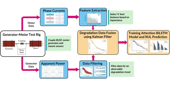
In this study, we proposed a fusion of degradation data to estimate the RUL of permanent magnet BLDC motors. Unlike other state-of-the-art techniques, we have taken into consideration two different crucial measurement points of the BLDC motor to estimate and predict its health states. These are phase currents () and output apparent power () of a coupled generator. 3-phase motor currents are acquired which are basically the inputs of motor. Apparent power computed from the coupled generator is considered as the output of the motor. A flowchart of the proposed method is presented in Figure 1. The proposed RUL estimation framework contains both the input characteristics as well as output characteristics of the motor, ensuring the highest form of reliability. This framework consists of mainly three steps.
Step 1: Degradation data: Four performance indices are computed from the motor phase currents which are selected based on a sensitivity score. Apparent power is computed from the three-phase generator currents and voltages through a moving average (MA) smoother function to acquire an observable degradation trend.
Step 2: RUL fusion: Degradation data from the two datasets are fused together using a Kalman filter (KF).
Step 3: RUL prediction: RUL prediction: A BiLSTM neural network model with an attention layer (ABLSTM) is trained using the degradation fusion from Step-2. The trained model is saved and tested using a different dataset containing different fault characteristics. Several performance measures are computed to validate the effectiveness of the RUL estimation.
2. Theoretical Overview
2.1. Electrical Signature Analysis (ESA)
In permanent magnet synchronous machines (PMSMs), electrical signatures hold a significant amount of fault related information. Usually, electrical waveforms contain phase, frequency, and amplitude related information of the system. Any form of deviation from these parameters will create an anomaly in the system, for example, excessive heat, sudden raise/drop in voltage, etc. Therefore, analyzing the electrical signals of the motor is necessary. Since we are focused on the SOH estimation of the BLDC motor, we have analyzed the electrical signatures of motor input currents. In the case of generator voltage, since it is driven by the motor’s output, total power generation is computed. Theoretical overview of ESA done in this study is presented below.
2.1.1. Normalized Modal Current Signature Analysis (NMCSA)
Electric motor’s phase currents carry significant fault-related information in presence of stator and rotor-related faults. Third harmonic (H3) analysis provides fault magnitude and fault frequency-related information in each motor phase. Practically, PMSMs have three-phase input currents where each current component is affected in the presence of a fault. Therefore, H3 analysis for all three current components needs to be done. This is time-consuming and computationally expensive. To overcome this drawback and make the FDI technique faster, we have used a normalized modal current (NMC) through a linear combination of 3-phase currents. Due to the linear combination, phase and frequency-related information of the original 3-phase currents are preserved. NMC computation is a two-step process as described below.
Step 1: The amplitude normalization is the first step in calculating the modal current. The magnitude of motor current varies greatly depending on the loads connected to it. Therefore, all three-phase currents should be expressed in a common normalized unit. As mentioned in [26], a simple signal processing technique is used to convert motor currents into a per unit () form.
where, is the normalized phase current, is the sensor acquired phase current, and , which stands for the phase current A, B, and C.
Step 2: Later, the normalized signals are linearized using (2) to obtain the modal current equation.
where, is the computed NMC, , , are normalized phase currents for Phase A, Phase B, and Phase C, respectively. Also, and are the modal current coefficients considered as 1, 2, and −3 [26,27].
The most significant aspect of NMC computation is that the original phase current characteristics (phase difference, frequencies, etc.) are preserved in the modal current due to the linear relationship. This will enable us to investigate the fault characteristics of each motor phase current without having to separately compute each phase signal.
Later, the NMCSA is performed in the frequency domain (F-D) and time-frequency domain (T-F-D) to observe the third harmonic components. Traditional fast Fourier transform (FFT) is used for the F-D analysis. For the T-F-D analysis, the continuous wavelet transform (CWT) method is used where the frequency is represented as a function of time. In the CWT method, the original time-series signal is convoluted with a short-duration wave-like function called a “mother wavelet” [28]. A generalized form of a mother wavelet function can be expressed as (3):
where, is the mother wavelet, and and are the scaling and translating parameters.
For a motor current signal, CWT transformation is done as shown in (4) [29]:
where, is the CWT representation of original current signal, . In this study, , computed using Equations (1) and (2).
2.1.2. Apparent Power
Fundamentally, apparent power is the combination of real power and reactive power in AC power systems. Real power is the power dissipation from the resistive components in a circuit, usually a DC circuit or an AC circuit where the impedance component is absent [30]. Reactive power is the power generated due to the presence of inductive or reactive load in an electrical circuit. Current and voltage of an AC circuit can be expressed as (5) and (6).
where, and are the peak current and peak voltage, respectively. is the angular frequency and is the phase difference. is the instantaneous power, computed using the instantaneous current, and instantaneous voltage, .
Using the trigonometric formula, , (7) can be re-written as:
where, is the part determines amplitude of the power, is the oscillating element and is the offset that indicates the phase difference between the current and voltage signals. If and are in phase, then , and the power becomes entirely resistive. Likewise, when the phase difference is maximum, then , and the power becomes entirely reactive [31]. Also, using the trigonometric formula, , (5) can be re-written as:
In that case, the power equation with the new current becomes:
First part of (11) is known as real power, P. And the second part is known as reactive power, Q. Combination of these two powers is called apparent power, S, which can be expressed as (12).
P, Q, and S can be expressed as a right-angle triangle where P and Q lie perpendicular to one another. A power triangle of P, Q, and S is shown in Figure 2.
2.2. Attention LSTM
Recurrent neural networks (RNNs) are evidently quite efficient in sequence modeling. Long short-term memory (LSTM) unit is a type of improved RNN with a long-term dependency that overcomes the vanishing gradient drawback of traditional RNNs [32]. Bidirectional LSTM (BiLSTM) cells create a network among the neurons of the previous layer as well as the next layer, enabling the flow of information in both directions [33]. From previous research, it is found out that BiLSTM algorithms have demonstrated better performance than the unidirectional LSTM models in sequence modeling.
An LSTM cell is made up of three gates that control the information flow throughout the network. Input, forget, and output gates are the three types of gates. The working theory of the LSTM is depicted in Figure 3. When the input gate is closed, inward information flow is disabled. Similarly, no information can come out of the cell if the output gate is turned off. Thus, by switching the gate operation, an LSTM can be activated and deactivated allowing the backpropagation algorithm to reach a long way without affecting the previously computed weights of LSTM cells [34]. BiLSTM network is a two-way LSTM information flow, therefore, the basic computation of the LSTM network remains the same in the BiLSTM network too. Some of the terminologies and mathematical computation of LSTM weights are:
here,
- used for updating
- input gate, forget gate, output gate
- weights. [* = input, forget, and output.]
Figure 3.
(a) A BiLSTM cell. (b) Representation of BiLSTM and ABLSTM training.

Weights computed from the BiLSTM layer are fed into the attention layer for further computation. The weight vector of BiLSTM layer can be expressed as . Then, the attention weights and vectors are computed using Equations (19) and (20) [35,36].
Here, is the weighted matrix obtained from LSTM layer output with associated bias vector, . is the attention weight vector and is the vector used for normalization. (*) is the activation function similar to the LSTM architecture [35,36,37]. Weighted time-step, is computed according to Equation (21) and output vector as Equation (22):
where . indicates the transpose of LSTM weight vector, .
2.3. Kalman Filter
In the engineering field, the Kalman filter (KF) uses a set of numerical computations, usually for a linear system, to provide an effective recursive solution using a series of measurements data. Based on the input and output response, KF can estimate the internal state through the comparison of analytical solution and predicted solution. The powerful aspect of this filter is to produce estimations future states, and it can also evaluate the precise nature of the modeled system when it is unknown [38]. The Kalman filter estimates a process by stating some time and obtaining the noisy measurements’ feedback to compare with the approximated time step. As a result, an update function for time and a prediction function for measurement are formed in a typical KF model. The time update functions are used to forecast the forward state which is known as predictor functions while the measurement update functions are responsible for the approximated historical state. Figure 4 shows the time update with approximated current state and the measurement update equation is used to update the previously approximated state ahead of current time [39].
The Kalman filter addresses the process by using the following framework and the model assumes the true state at time k is progressed from the previous state at (k − 1) according to Equation (23):
where, is the state transition model, is the previous state, is the control-input model, is the control vector; is the process noise. Equation (24) shows that an observation can be made at time using the true state ,
where is the observation model and is the observation noise. Both and are said to follow the Gaussian distribution [38,39,40].
Thus, a KF model can be used to obtain a fused degradation pattern by combining two or more degradation data with same measurement points. To combine the data, one of the series should be considered a time function and based on the rest of the data, a new state is estimated through continuous multiple updating. A noise matrix can be formed based on the type of problem and data structure. Typically, variance of the signal can be multiplied with its data points to obtain a noisy measurement. Or, Gaussian white noise can be used directly to obtain a noisy measurement that follows the Gaussian distribution.
3. Test Rig and Data Description
3.1. Experiment Setup
To acquire data for this study, BLDC motors are used with generators to create a generator-motor (G-M) test rig. A motor is connected to a generator through a spider-type coupling where the shafts of the motor and generator are coupled. A picture of the original test bench is presented in Figure 5a and a schematic with component blocks is shown in Figure 5b. The reason we selected a G-M setup is the simplicity in building, controlling, and acquiring experimental data [41]. In G-M set operation, generator’s shaft rotation is driven by the torque applied by the coupled BLDC motor. Therefore, the electrical energy induced in the generator phase is a result of the motor’s output, which can be used to analyze the motor’s health state efficiently. Motor and generator used in this study are of the same type (BLDC) and purchased from the same manufacturer (DNJ Korea) to minimize the inconsistency in energy conversion. A detailed listing of the motor parameters is presented in Table 1. A generator with higher power rating (40 W) is used with the motor (26 W) to make sure there is no power loss of disturbances through the generator when the motor operates at maximum speed.
The major feature that distinguishes a BLDC motor from a conventional DC motor is the lack of a mechanical commutator or brush. Thus, a BLDC motor can deliver higher torque than that of a brushed or conventional DC motor. Also, BLDC motor is prioritized over conventiona DC motor due to its precise control, high efficacy, silent operation, higher torque-to-body ratio, and prolonged lifespan [42]. Nevertheless, BLDC motor control phenomenon is complicated and often requires an external driver to control electromagnetic induction. In literature there are number of studies on the control strategies of BLDC motors such as—external driver, sensorless control, proportional integral derivative (PID) tuned control, comparator assisted control, etc. [42,43,44]. We have used an LBD-V4 motor driver to control the BLDC motor. The motor driver receieves a 24.0 V constant DC voltage and converts it into a pulse width modulation (PWM) signal with a 50% duty cycle. The Pole position of the permanent magnet (rotor) is identified using a set of hall effect sensors (HES). A temporary magnet with N pole and S pole are created using phase current flow through the stoator coils. These pole positions are continously altereted by changing the polarity of motor’s phase current. Thus, the rotor never aligns with the staotor position and keeps on rotating.
Data acquisition (DAQ) environment is set up using an apparatus from national instruments (NI). A DAQ chassis, NI cDAQ-9178, is used with different modules to acquire different sensor data such as NI-9246, NI-9205, and NI-9214 for current, voltage, and temperature, respectively. In this study, four different sensor data were monitored continuously during the motor test. These are motor current, generator voltage, stator temperature, and motor speed. The sampling rate for current and voltage acquisition was set to be 5.0 kHz and for temperature it was 100 Hz. LabVIEW software is used to set different DAQ parameters, control the sensor sensitivity, and store the data in a computer.
3.2. Failure Modes
Electromagnetic induction of the BLDC motor is mainly done by changing the polarity and magnitude of current passing through the stator coils. From the signals of HES, the motor driver converts the stator coils into temporary electromagnets with different pole position based on current polarity. A circuit of transistors controls the PWM output of the motor driver through a fast switching between ON and OFF states. The commutation logic for the BLDC motor operation is shown in Table 2. It is understandable that an irregularity in stator operation will largely affect the entire operation of the BLDC motor. Therefore, in this study, we have focused on two most commonly occurring faults in stator coil with three different datasets. These are:
- (1)
- Dataset-1: An inter-turn short-circuit is created at the stator coil winding as shown in the B2’ winding in Figure 6a. This fault generates two different impedances on the coil winding creating a disturbance in current flow. It is also called a turn-to-turn fault where a short-circuit is produced in two sections of the stator coil. This type of fault is labeled “ITF fault” which is illustrated in Figure 6a.
- (2)
- Dataset-2: In this type of fault, two adjacent windings are shorted. This type of fault is labeled as a winding short-circuit (WSC) fault. Figure 6b shows a winding short-circuit fault where Phase A and Phase C are shorted together through the windings A1 and C2′. In this paper, this type of setting is labeled “WSC fault”.
- (3)
- Dataset-3: This dataset consists of data from a motor with both ITF and WSC fault generated on the stator at the same time. This type of scenario is labeled “Hybrid fault”.
4. RUL Prediction
4.1. ESA
Two different electrical data are acquired from the G-M test setup. The first one is the input phase current (I) of the BLDC motor. This measurement is conducted through the motor driver to BLDC motor stator connections which is the three-phase input of the motor. Another current is measured from the three-phase output terminals of the generator. The second sensor data acquired is the voltage (V). Like the current measurement, voltage is measured from the input phases of the motor and output phases of the generator. Sensor acquired I-V signals are shown in Figure 7. Input voltage is a PWM-type signal with a 50% duty cycle and the input voltage is distorted due to the failure in the motor and loads connected to the generator. On the other hand, output voltages and currents acquired from the generator follow a three-phase sinusoidal waveform shape. As mentioned in previous sections, motor current signature analysis (MCSA) is an effective method for fault detection and isolation in PMSMs. Stator coils are arranged in a STAR configuration where all the phase connections have a common terminal. According to Kirchhoff’s current law (KCL), no current should flow through this common terminal. Using the harmonic analysis of the motor current, we can understand if there is any current flowing through that common node. Every third harmonic presented in the current signature indicates the deviation from the KCL. Therefore, through the fast Fourier transform (FFT) analysis we can isolate the magnitude of the third harmonic component as well as the harmonic frequency range. However, analyzing all the three-phase currents is time-consuming and computationally expensive. This is why, in this study we have used a normalized modal current analysis (NMCA) approach for fast decision making. Computation of normalized modal current (NMC) is mathematically shown in Equation (2) and the representation of three-phase currents and corresponding NMC is shown in Figure 8. Three-phase current is expressed in Amperes (A) and NMC is expressed per unit () due to the linear conversion. Third harmonic analysis using the NMC is presented in Figure 9. The first column is the NMC signals in time domain, and the second and third columns are the frequency domain and time-frequency domain, representations, respectively. From the top, each row represents NMC in healthy state, ITF fault state, WSC fault state, and hybrid fault state, subsequently. It can be seen that a larger peak is present for all types of NMC at around 250 Hz which is the fundamental frequency (fn) of the signals. Apart from these, other frequency components are denoted as first, second, and third harmonics. In this paper, each third sequence harmonic component (i.e., third, sixth, ninth …… etc.) is referred to as first, second, third ……etc. orders. For example, in case of healthy current NMC, no third harmonic component is seen. However, in case of all the fault cases, two third harmonic components at the third sequence and sixth sequence are observed. CWT analysis shows a better representation of the third harmonic component with abrupt changes in time-frequency scalogram. A list of NMCSA result is presented in Table 3.
Sensor acquired signals as well as the NMC are necessarily time-series data and analysis from multiple domains is necessary to make a decision. Therefore, we have extracted a range of statistical features from the NMC. A list of features is presented in Table 4 and a detailed description of the features can be found in reference [17,29,41]. Working with all these features can lead to overfitting phenomena in deep learning algorithms. To avoid the curse of higher dimensions, we have selected two best features from the time domain and two best features from the frequency domain. Feature selection approach consists of building a sensitivity index called σ.
This index is computed from three different factors named analysis of variance test, monotonicity, and Kruskal-Wallis variance test scores as expressed in Equation (25):
where:
- = The ratio of the variance calculated among the means to the variance within the features, which is computed using the analysis of variance (ANOVA) test.
- = A measure of feature’s prognostibility.
- = Measures the stochastic dominance of to one another.
The standing of the features with individual index scores is shown in Figure 10. As the fault becomes severe, these features show variable trends in its characteristics. For the three fault scenarios analyzed in this study, the BLDC motor lasted for 1750 h in case of ITF fault, 2230 h for WSC fault, and 1450 for hybrid fault. Feature trends for the entire lifecycle of the BLDC motor are shown in Figure 11. It is seen that RSSQ, VAR, and H3 have an increasing trend as the fault propagates, whereas RVF has a degradation trend as the motor reaches a more severe condition.
4.2. Apparent Power Degradation Data
Generator output signals are acquired through a resistive-inductive-capacitive (RLC) circuit. Due to the presence of resistive and inductive loads, generator power consists of both the real power (P) and reactive power (Q). After acquiring the I-V signals, we have computed the apparent power of the generator using Equation (11). As the motor degrades through time, its torque reduces, and power generated at the generator end also drops down. The power trend for different fault states is shown in Figure 12. Sensor acquired signals consist of noise and undiscernible degradation trend. To get a noiseless observable trend, we have used a moving-average (MA) filter. MA performed on power data can be expressed mathematically in Equation (26).
Here, is the sum of voltages at instances, respectively. is the number of order MA computations.
4.3. RUL Fusion and Prediction
After acquiring and filtering the power degradation data, ITF fault data (Dataset-1) and WSC fault data (Dataset-2) are fused using a Kalman filter. The output of fused RUL is shown in Figure 13. The fused RUL has a service time of 2004 h after filtering. This fused RUL is used to train the proposed attention-based bidirectional LSTM (ABLSTM) model. Raw data normalization is a common method used in machine learning for improving model accuracy. According to their needs, many researchers have used this method to scale data within a boundary with a defined set of ranges. Normalization suppresses the outliers and reduces standard deviation in train data making it suitable for the algorithm to learn in a faster way. We have used a min-max scaler and scaled the power data in a range of 0–1. Since the RUL is mainly concerned with estimating the beginning of life (BOL) and end of life (EOL), a percent scale of power data with 0% represents EOL and 100% represents the BOL. Apparent power normalization using min-max scaler is shown in Equation (27):
Ssc is the scaled apparent power after min-max scaling. and refers to the maximum and minimum power, respectively. is the voltage at ith instance.
ABLSTM model consists of an attention layer with BiLSTM cells. The number of hidden layers selected for the model is two, with each layer containing 512 neurons. Since we used a large number of neurons, the model may become overfitted, which is a normal occurrence in neural networks. To prevent overfitting, we used a regularization approach called “Dropout,” which removes some activations of the previous layer neurons from the network and ignores them during the training stage. During testing, these randomly dropped neurons reactivate and contribute to model learning. A list of model parameters is presented in Table 5.
Fused RUL from the KF algorithm is used as the training data of the model. After the training, the model was saved in the computer with associated weights. Later, the trained model is used to predict the RUL of hybrid fault data. To compare the efficacy of the ABLSTM model, two other DL models are trained and tested using the same datasets. The other two models are artificial neural networks (ANN) and regular LSTM networks. RUL prediction results for all the NN models are shown in Figure 14.
4.4. Validation
As seen in Figure 13, all the models perform quite well in predicting hybrid fault RUL. However, because of the attention mechanism in the abruptly changing power degradation trend, ABLSTM shows a better prediction result compared to others. Even for a very small degradation trend, ABLSTM has attained the variation and predict appropriately. To better understand the model performance, two regression metrics are obtained which are root mean squared error (RMSE) and mean absolute error (MAE). These metrics can be described mathematically as Equations (28) and (29). Another metric named is further computed from the model’s predicted RUL and actual RUL to compute the RUL prediction error. Mathematical expression of is shown in Equation (30) and computed for RULs are presented in Table 6.
here:
- = actual power data
- = predicted power data by the models
- = The total number of data
Computed RMSE and MAE scores of the models are represented in a percentage scale as shown in Figure 15. The proposed ABLSTM model has a lower error compared to regular LSTM, BiLSTM, and ANN models. However, the computational time for the ABLSTM model is higher compared to other models due to the attention mechanism. Therefore, for a dataset with no abruptly changing behavior, the BiLSTM model can be used instead of the ABLSTM model to reduce the computation time. These deep learning models were trained on a computer with an AMD Ryzen 7 2700 octa-core CPU and 32 GB of RAM. An NVIDIA GTX 970 GPU with 4 GB VRAM is used for accelerated computation. Python language is used with open-source deep learning platform, Tensorflow and Keras for the deep neural networks.
5. Conclusions
A data-driven RUL estimation framework of the BLDC motor is presented in this paper using the electrical I-V characteristics. Input current signals from the BLDC motor and coupled generator’s output apparent power are analyzed and fused to estimate the RUL. Instead of a three-phase motor current analysis, a normalized modal current (NMC) is used for the fault detection and feature extraction. Due to the presence of reactive load on the generator side, a reactive power (Q) is produced along with the real power (P). Using the I-V characteristics of the generator output, apparent power (S) is computed which is the combination of P and Q. Three different failure cases are analyzed which are obtained from three different accelerated life tests. Three faults are: inter-turn short-circuit (ITF), winding short-circuit (WSC), and hybrid (combination of ITF and WSC). ITF and WSC degradation data are fused using a Kalman filter to acquire a fused RUL. This fused RUL is trained in an attention-based bidirectional LSTM (ABLSTM) neural network. Later, the trained ABLSTM was used to predict the trend of hybrid RUL along with three other neural networks (NN) models. The performance of the NN models is evaluated using different metrics. It is found out that ABLSTM outperforms other NN models in terms of RUL prediction.
Adoption of electrical parameters for maintenance decision making is quite efficient compared to other traditional methods as in electric motors, I-V characteristics changes at the incipient stage of a failure. Analysis of I-V characteristics will provide a robust PHM framework of BLDC motor as well as other PMSMs. This study can be further extended for a real-time updating method to enable online RUL estimation of electric motors. Also, physics-of-failure models can be combined with the proposed method to establish a hybrid PHM framework of electric motors.
Author Contributions
Conceptualization, T.A.S. and R.Y.; methodology, T.A.S.; software, T.A.S.; validation, J.-W.H. and T.A.S.; formal analysis, R.Y.; investigation, J.-W.H.; resources, T.A.S.; data curation, T.A.S.; writing—R.Y.; writing—review and editing, T.A.S. and R.Y.; visualization, R.Y.; supervision, J.-W.H.; project administration, J.-W.H.; funding acquisition, J.-W.H. All authors have read and agreed to the published version of the manuscript.
Funding
This work was supported by the National Research Foundation of Korea (NRF) funded by the Ministry of Science and ICT (MSIT), Korea Government under Grant 2019R1/1A3A01063935.
Institutional Review Board Statement
Not applicable.
Informed Consent Statement
Not applicable.
Data Availability Statement
Data available on request.
Conflicts of Interest
The authors declare no conflict of interest.
References
- Kim, N.-H.; An, D.; Choi, J.-H. Prognostics and Health Management of Engineering Systems; Springer International Publishing: Basel, Switzerland, 2017; pp. 18–185. [Google Scholar]
- Pecht, M.G.; Kang, M. (Eds.) Prognostics and Health Management of Electronics: Fundamentals, Machine Learning, and the Internet of Things; John Wiley & Sons: Hoboken, NJ, USA, 2018; pp. 5–72. [Google Scholar]
- Lei, Y. Intelligent Fault Diagnosis and Remaining Useful Life Prediction of Rotating Machinery; Butterworth-Heinemann: Oxford, UK, 2016; pp. 12–86. [Google Scholar]
- Nandi, S.; Toliyat, H.A.; Li, X. Condition Monitoring and Fault Diagnosis of Electrical Motors—A Review. IEEE Trans. Energy Convers. 2005, 20, 719–729. [Google Scholar] [CrossRef]
- Loutas, T.H.; Roulias, D.; Georgoulas, G. Remaining useful life estimation in rolling bearings utilizing data-driven probabilistic e-support vectors regression. IEEE Trans. Reliab. 2013, 62, 821–832. [Google Scholar] [CrossRef]
- Medjaher, K.; Tobon-Mejia, D.A.; Zerhouni, N. Remaining Useful Life Estimation of Critical Components with Application to Bearings. IEEE Trans. Reliab. 2012, 61, 292–302. [Google Scholar] [CrossRef] [Green Version]
- Peng, Y.; Hou, Y.; Song, Y.; Pang, J.; Liu, D. Lithium-Ion Battery Prognostics with Hybrid Gaussian Process Function Regression. Energies 2018, 11, 1420. [Google Scholar] [CrossRef] [Green Version]
- Djeziri, M.A.; Benmoussa, S.; Zio, E. Review on Health Indices Extraction and Trend Modeling for Remaining Useful Life Estimation. In Artificial Intelligence Techniques for a Scalable Energy Transition; Springer Science and Business Media LLC: Cham, Switzerland, 2020; pp. 183–223. [Google Scholar]
- Si, X.-S.; Wang, W.; Hu, C.-H.; Zhou, D.-H. Remaining useful life estimation—A review on the statistical data driven approaches. Eur. J. Oper. Res. 2011, 213, 1–14. [Google Scholar] [CrossRef]
- Caesarendra, W.; Tjahjowidodo, T. A review of feature extraction methods in vibration-based condition monitoring and its application for degradation trend estimation of low-speed slew bearing. Machines 2017, 5, 21. [Google Scholar] [CrossRef]
- Randall, R.B. Vibration-Based Condition Monitoring: Industrial, Automotive and Aerospace Applications; John Wiley & Sons: Hoboken, NJ, USA, 2021; pp. 86–318. [Google Scholar]
- Moshrefzadeh, A. Condition monitoring and intelligent diagnosis of rolling element bearings under constant/variable load and speed conditions. Mech. Syst. Signal Process. 2021, 149, 107153. [Google Scholar] [CrossRef]
- Candelo-Zuluaga, C.; Riba, J.-R.; López-Torres, C.; Garcia, A. Detection of Inter-Turn Faults in Multi-Phase Ferrite-PM Assisted Synchronous Reluctance Machines. Energies 2019, 12, 2733. [Google Scholar] [CrossRef] [Green Version]
- Garcia-Calva, T.; Morinigo-Sotelo, D.; Fernandez-Cavero, V.; Garcia-Perez, A.; Romero-Troncoso, R. Early Detection of Broken Rotor Bars in Inverter-Fed Induction Motors Using Speed Analysis of Startup Transients. Energies 2021, 14, 1469. [Google Scholar] [CrossRef]
- Yang, F.; Habibullah, M.S.; Zhang, T.; Xu, Z.; Lim, P.; Nadarajan, S. Health Index-Based Prognostics for Remaining Useful Life Predictions in Electrical Machines. IEEE Trans. Ind. Electron. 2016, 63, 2633–2644. [Google Scholar] [CrossRef]
- Strangas, E.G.; Aviyente, S.; Zaidi, S.S.H. Time–Frequency Analysis for Efficient Fault Diagnosis and Failure Prognosis for Interior Permanent-Magnet AC Motors. IEEE Trans. Ind. Electron. 2008, 55, 4191–4199. [Google Scholar] [CrossRef]
- Alam Shifat, T.; Hur, J.-W. ANN Assisted Multi Sensor Information Fusion for BLDC Motor Fault Diagnosis. IEEE Access 2021, 9, 9429–9441. [Google Scholar] [CrossRef]
- Alam Shifat, T.; Jang-Wook, H. Remaining Useful Life Estimation of BLDC Motor Considering Voltage Degradation and Attention-Based Neural Network. IEEE Access 2020, 8, 168414–168428. [Google Scholar] [CrossRef]
- Krichen, M.; Elbouchikhi, E.; Benhadj, N.; Chaieb, M.; Benbouzid, M.; Neji, R. Motor Current Signature Analysis-Based Permanent Magnet Synchronous Motor Demagnetization Characterization and Detection. Machines 2020, 8, 35. [Google Scholar] [CrossRef]
- Alam Shifat, T.; Hur, J.-W. An Effective Stator Fault Diagnosis Framework of BLDC Motor Based on Vibration and Current Signals. IEEE Access 2020, 8, 106968–106981. [Google Scholar] [CrossRef]
- Cruz, S.; Cardoso, A. Stator winding fault diagnosis in three-phase synchronous and asynchronous motors, by the extended Park’s vector approach. IEEE Trans. Ind. Appl. 2001, 37, 1227–1233. [Google Scholar] [CrossRef]
- Zafarani, M.; Bostanci, E.; Qi, Y.; Goktas, T.; Akin, B. Interturn Short-Circuit Faults in Permanent Magnet Synchronous Machines: An Extended Review and Comprehensive Analysis. IEEE J. Emerg. Sel. Top. Power Electron. 2018, 6, 2173–2191. [Google Scholar] [CrossRef]
- Drif, M.; Cardoso, A.J.M. Stator Fault Diagnostics in Squirrel Cage Three-Phase Induction Motor Drives Using the Instantaneous Active and Reactive Power Signature Analyses. IEEE Trans. Ind. Inform. 2014, 10, 1348–1360. [Google Scholar] [CrossRef]
- Faiz, J.; Moosavi, S.M.M. Detection of mixed eccentricity fault in doubly-fed induction generator based on reactive power spectrum. IET Electr. Power Appl. 2017, 11, 1076–1084. [Google Scholar] [CrossRef]
- Ehsanifar, A.; Allahbakhshi, M.; Tajdinian, M.; Dehghani, M.; Montazeri, Z.; Malik, O.; Guerrero, J.M. Transformer inter-turn winding fault detection based on no-load active power loss and reactive power. Int. J. Electr. Power Energy Syst. 2021, 130, 107034. [Google Scholar] [CrossRef]
- Jafari, A.; Faiz, J.; Jarrahi, M.A. A Simple and Efficient Current Based Method for Inter-turn Fault Diagnosis of Brush-less Direct Current Motors. IEEE Trans. Ind. Inform. 2020, 17, 2707–2715. [Google Scholar] [CrossRef]
- Perera, N.; Rajapakse, A.D.; Buchholzer, T.E. Isolation of faults in distribution networks with distributed generators. IEEE Trans. Power Deliv. 2008, 23, 2347–2355. [Google Scholar] [CrossRef]
- Guo, M.-F.; Zeng, X.-D.; Chen, D.-Y.; Yang, N.-C. Deep-Learning-Based Earth Fault Detection Using Continuous Wavelet Transform and Convolutional Neural Network in Resonant Grounding Distribution Systems. IEEE Sens. J. 2018, 18, 1291–1300. [Google Scholar] [CrossRef]
- Alam Shifat, T.; Hur, J.-W. EEMD assisted supervised learning for the fault diagnosis of BLDC motor using vibration signal. J. Mech. Sci. Technol. 2020, 34, 3981–3990. [Google Scholar] [CrossRef]
- Grigsby, L.L. Electric Power Generation, Transmission, and Distribution; CRC Press: Boca Raton, FL, USA, 2018; pp. 18–230. [Google Scholar]
- Hubert, C.I. Electric Machines: Theory, Operation, Applications, Adjustment, and Control; Pearson Education: Upper Saddle River, NJ, USA, 2002; pp. 68–334. [Google Scholar]
- Zhang, J.; Wang, P.; Yan, R.; Gao, R.X. Long short-term memory for machine remaining life prediction. J. Manuf. Syst. 2018, 48, 78–86. [Google Scholar] [CrossRef]
- Yao, J.; Jiang, X.; Wang, S.; Jiang, K.; Yu, X. SVM-BiLSTM: A Fault Detection Method for the Gas Station IoT System Based on Deep Learning. IEEE Access 2020, 8, 203712–203723. [Google Scholar]
- Ng, A. CS229 Course Notes: Deep Learning; Stanford University: Stanford, CA, USA, 2018. [Google Scholar]
- Mamo, T.; Wang, F.-K. Long Short-Term Memory with Attention Mechanism for State of Charge Estimation of Lithium-Ion Batteries. IEEE Access 2020, 8, 94140–94151. [Google Scholar] [CrossRef]
- Zhou, H.; Zhang, Y.; Yang, L.; Liu, Q.; Yan, K.; Du, Y. Short-Term Photovoltaic Power Forecasting Based on Long Short Term Memory Neural Network and Attention Mechanism. IEEE Access 2019, 7, 78063–78074. [Google Scholar] [CrossRef]
- Chen, Z.; Wu, M.; Zhao, R.; Guretno, F.; Yan, R.; Li, X. Machine Remaining Useful Life Prediction via an Attention-Based Deep Learning Approach. IEEE Trans. Ind. Electron. 2020, 68, 2521–2531. [Google Scholar] [CrossRef]
- Bishop, G.; Welch, G. “An Introduction to the Kalman Filter.” Proc of SIGGRAPH, Course 8.27599-23175 (2001): 41. Available online: http://132.206.230.228/e761/SIGGRAPH2001_CoursePack_08.pdf (accessed on 1 May 2021).
- Huang, S.; Tan, K.K.; Lee, T.H. Fault Diagnosis and Fault-Tolerant Control in Linear Drives Using the Kalman Filter. IEEE Trans. Ind. Electron. 2012, 59, 4285–4292. [Google Scholar] [CrossRef]
- Foo, G.H.B.; Zhang, X.; Vilathgamuwa, D.M. A Sensor Fault Detection and Isolation Method in Interior Permanent-Magnet Synchronous Motor Drives Based on an Extended Kalman Filter. IEEE Trans. Ind. Electron. 2013, 60, 3485–3495. [Google Scholar] [CrossRef]
- Hur, J.-W.; Alam, T. Motor vibration analysis for the fault diagnosis in nonstationary operating conditions. Int. J. Integr. Eng. 2020, 12, 151–160. [Google Scholar]
- Kim, S.H. Electric Motor Control: DC AC and BLDC Motors; Elsevier: Amsterdam, The Netherlands, 2017. [Google Scholar]
- Yedamale, P. Brushless DC (BLDC) Motor Fundamentals; Microchip Technology Inc.: Chandler, AZ, USA, 2003; Volume 20, pp. 3–15. [Google Scholar]
- Kandiban, R.; Arulmozhiyal, R. Speed control of BLDC motor using adaptive fuzzy PID controller. Procedia Eng. 2012, 38, 306–313. [Google Scholar] [CrossRef] [Green Version]
Figure 1.
Graphical illustration of the proposed RUL estimation method.

Figure 2.
Power triangle of AC power system.

Figure 4.
Updating of Kalman Filter.

Figure 5.
Test rig setup. (a) Reat test bench photo, (b) Schematic diagram of the test bench setup.

Figure 6.
(a) Inter-turn short circuit fault. (b) Winding short-circuit fault.

Figure 7.
Sensor acquired current and voltage signals. (a) Motor current (input), (b) Generator current (output), (c) Motor voltage (input), (d) Generator voltage (output).
Figure 7.
Sensor acquired current and voltage signals. (a) Motor current (input), (b) Generator current (output), (c) Motor voltage (input), (d) Generator voltage (output).

Figure 8.
Modal current computation from the three-phase motor current.

Figure 9.
Third harmonic (H3) analysis of the motor currents in healthy state (row A), ITF fault state (row B), WSC fault state (row C), hybrid fault state (row D). Column X is the sensor acquired time series signal, column Y is the FFT transformation, column Z is the time-frequency representation using CWT.

Figure 10.
(a) Time domain features. (b) Frequency domain features.

Figure 11.
Feature trends for different faults. (a) Inter-turn short circuit fault. (b) Winding short-circuit fault, (c) Hybrid fault.
Figure 11.
Feature trends for different faults. (a) Inter-turn short circuit fault. (b) Winding short-circuit fault, (c) Hybrid fault.

Figure 12.
Degradation data of different fault states. (a) ITF fault, (b) WSC fault, (c) Hybrid fault.
Figure 12.
Degradation data of different fault states. (a) ITF fault, (b) WSC fault, (c) Hybrid fault.

Figure 13.
RUL estimation from ITF and WSC degradation data.

Figure 14.
Prediction result of BiLSTM model on hybrid fault dataset.

Figure 15.
Performance comparison among different models.


Table 1.
BLDC motor parameters.
| Parameter | Measurement |
|---|---|
| Motor model | BLS-24026N |
| Generator model | BLS-24040N |
| Input Parameters | 24.0 VDC & 7.0 A (max) |
| Current module | NI 9246 |
| Voltage module | NI 9203, NI 9205 |
| Temperature module | NI 9214 |
| Electrical load | 10 MΩ DELTA |
| Motor’s Power(rated) | 26 W |
| Generator Power(rated) | 40 W |
| Shaft Speed (rated) | 4000 RPM |
| Sampling Frequency (Voltage, Current) | 5 kHz |
Table 2.
Commutation of BLDC Motor.
| Motor Phase | Commutation Logic | ||||||||
|---|---|---|---|---|---|---|---|---|---|
| Step | A | B | C | AH | AL | BH | BL | CH | CL |
| 01 | + | - | OFF | 1 | 0 | 0 | 1 | 0 | 0 |
| 02 | + | OFF | - | 1 | 0 | 0 | 0 | 0 | 1 |
| 03 | OFF | + | - | 0 | 0 | 1 | 0 | 0 | 1 |
| 04 | - | + | OFF | 0 | 1 | 1 | 0 | 0 | 0 |
| 05 | - | OFF | + | 0 | 1 | 0 | 0 | 1 | 0 |
| 06 | OFF | - | + | 0 | 0 | 0 | 1 | 1 | 0 |
Table 3.
NMCSA results.
| NMC Parameters | Amplitudes and Frequency Band | |||||||
|---|---|---|---|---|---|---|---|---|
| Healthy | ITF Fault | WSC Fault | Hybrid Fault | |||||
| f(Hz) | |INMC| | f(Hz) | |INMC| | f(Hz) | |INMC| | f(Hz) | |INMC| | |
| fn | 238 | 4.21 | 330 | 3.20 | 275 | 2.71 | 210 | 2.08 |
| First H3 | - | - | 1118 | 0.92 | 1009 | 0.71 | 997 | 0.43 |
| Second H3 | - | - | 1580 | 0.23 | 1630 | 0.20 | 1610 | 0.23 |
Table 4.
Features computed in different dimensions.
| Domains | Feature Names |
|---|---|
| Time Domain | Peak-to-Peak (P2P), Root Sum of Squares (RSSQ), Variance (VAR),FM4, FM8, M6A, Skewness (SKEW), L1 Norm (L1), L2 Norm (L2), Peak to RMS (P2RMS), Crest Factor (CF), Shape Factor (SF), Margin Factor (MF), Clearance Factor (CLF). |
| Frequency Domain | Peak Frequency (PF), Total Harmonic Distortion (THD), Spectral Skewness (SS), Mean frequency (MF), 3rd harmonic magnitude (H3), Entropy, Root Variance Frequency (RVF). |
Table 5.
Model Parameters used for RUL Prediction.
| Parameter | Value |
|---|---|
| RNN Cell | BiLSTM |
| Hidden Layers | 2 |
| Optimizer | Adam |
| Dropout | 0.15 |
| Neurons | 512, 512 |
| Loss Function | MAE |
| Epochs | 1000 |
| Activation | ReLU |
Table 6.
Standard Deviation of RUL Prediction Errors.
| Dataset Size | ANN | LSTM | BiLSTM | ABLSTM |
|---|---|---|---|---|
| 25% | 0.037 | 0.025 | 0.021 | 0.016 |
| 50% | 0.033 | 0.018 | 0.019 | 0.011 |
| 75% | 0.027 | 0.193 | 0.18 | 0.012 |
| 100% | 0.031 | 0.24 | 0.20 | 0.014 |
Publisher’s Note: MDPI stays neutral with regard to jurisdictional claims in published maps and institutional affiliations. |
© 2021 by the authors. Licensee MDPI, Basel, Switzerland. This article is an open access article distributed under the terms and conditions of the Creative Commons Attribution (CC BY) license (https://creativecommons.org/licenses/by/4.0/).
Share and Cite
MDPI and ACS Style
Shifat, T.A.; Yasmin, R.; Hur, J.-W. A Data Driven RUL Estimation Framework of Electric Motor Using Deep Electrical Feature Learning from Current Harmonics and Apparent Power. Energies 2021, 14, 3156. https://doi.org/10.3390/en14113156
AMA Style
Shifat TA, Yasmin R, Hur J-W. A Data Driven RUL Estimation Framework of Electric Motor Using Deep Electrical Feature Learning from Current Harmonics and Apparent Power. Energies. 2021; 14(11):3156. https://doi.org/10.3390/en14113156
Chicago/Turabian StyleShifat, Tanvir Alam, Rubiya Yasmin, and Jang-Wook Hur. 2021. "A Data Driven RUL Estimation Framework of Electric Motor Using Deep Electrical Feature Learning from Current Harmonics and Apparent Power" Energies 14, no. 11: 3156. https://doi.org/10.3390/en14113156
Note that from the first issue of 2016, this journal uses article numbers instead of page numbers. See further details here.