A Forecast-Based Load Management Approach for Commercial Buildings Demonstrated on an Integration of BEV

Abstract

Load-forecasting problems have already been widely addressed with different approaches, granularities and objectives. Recent studies focused not only on deep learning methods but also on forecasting loads on single building level. This study aims to research problems and possibilities arising by using different load-forecasting techniques to manage loads. For that behavior of two neural networks, Long Short-Term Memory and Feed-Forward Neural Network as well as two statistical methods, standardized load profiles and personalized standardized load profiles are analyzed and assessed by using a sliding-window forecast approach. The results show that personalized standardized load profiles (MAE: 3.99) can perform similar to deep learning methods (for example, LSTM MAE: 4.47). However, because of the simplistic approach, load profiles are not able to adapt to new patterns. As a case study for evaluating the support of load-forecasting for applications in energy management systems, the integration of charging stations into an existing building is simulated by using load-forecasts to schedule the charging procedures. It is shown that forecast- based controlled charging can have a significant impact by lowering overload peaks exceeding the house connection point power limit (controlled charging 20.24 kW; uncontrolled charging: 65.15 kW) while slightly increasing average charging duration. It is concluded that integration of high flexible loads can be supported by using forecast-based energy management systems with regards to their limitations.

1. Introduction

The on-going energy system transformation process, intended to reduce CO₂ emissions and meet the EU’s long-term goal of being climate-neutral by 2050, is shifting the dependence of energy production from fossil fuels to renewable energy sources such as wind and solar energy. This also leads to the integration of the three main energy sectors into buildings: electricity, heat and transport. For this reason, new challenges arise for electricity grids. As far as energy production is concerned, the increasing share of renewable energy sources and the resulting dependency on them [1] introduces uncertainties into power generation [2].

A further problem for electricity grids arises from the electrification of the transport sector through increasing overall electricity consumption and with charging times overlapping with periods of high peak loads [3]. It is expected that the charging of electric cars will have an effect on the general network stability in Germany with a share of 10–20%. However, due to the expected peak loads, a load management system can avoid overloading the grid connection point or the upstream transformer [4]. As an example, the integration of charging infrastructure for battery-electric vehicles (BEVs) into the existing building stock will create high demand for load management in order to avoid infrastructure extension.

One solution for increasing grid stability when integrating charging facilities for BEVs into existing buildings can be a load-forecast-based load management system. With such a system, charging processes can be scheduled and, e.g., shifted to times when building load balances fit power restrictions. From the view of an electric utility, such a system also enables the shifting of loads to beneficial times when the consumer participates in demand response tariffs [5].

This paper presents an approach to assess the behavior of load-forecasting techniques and investigates the capabilities of using deep learning techniques for load management applications. For that, basic Long Short-Term Memory and Feed-Forward Neural Networks models are optimized and trained in a sliding window forecasting framework as used and proposed by Bedi et al. [6] The forecasting results are compared to statistical methods’ standardized load profiles and personalized standardized load profiles, operationally used for grid management in Germany, to quantify problems and advantages of the different methods in their forecasting behavior and accuracy. Widely approved and important features were used to derive the models for the neural networks. Weather parameters such as temperature, humidity and wind speed were shown to be important and widely used variables [7,8]. The ambient air temperature, for example, has a high correlation with the load measurements of a building, while humidity also has a direct impact on people’s energy consumption behavior in buildings, such as the need for increased cooling demand [9]. Calendar effects as, for instance, indicators for the day or time are also used, but tend to have a low impact on the outcome [10]; also because of the arising possibility of using data with higher resolution opened by smart metering systems, the granularity of the data is lowered to a 5 min resolution scale. Combining the sliding window and the decrease of granularity allows the exploration of load-forecasting-based load management systems in more detail.

The forecast accuracy was measured by different commonly used absolute metrics, such as Mean Absolute Error (MAE) and Root Mean Squared Error (RMSE), and normalized metrics, e.g., Mean Absolute Percentage Error (MAPE) (used, for example, by Hossen et al. [11] and Fen et al. [12]); also in this study, the more recently introduced Mean Absolute Scaled Error (MASE) described by Hyndman et al. [13] is used.

The necessity of forecast-based load management was discussed in a case study. Therefore, integration of a varying number of BEVs with different charging behaviors and a fixed power limit in the building were simulated and evaluated. It shows the possibility of integrating a larger amount of charging infrastructure into existing commercial buildings by applying forecast-based charging strategies.

The key contributions of this paper are:

• Simulated usage of deep neural network for building level load-forecasting on 5 min granularity for load management applications.
• Quantify the performance of these models and compare them to standardized load profile techniques concerning their forecasting capabilities and behavior towards load management applications.
• Case study of integration of electric vehicles into an existing commercial building.
• Load management: Comparison between unscheduled and forecast-based BEV charging.

The article is structured as follows: In Section 2, a literature review is presented to determine the currently used approaches in load-forecasting, followed by Section 3, in which the general methodology is described to assess the chosen algorithms. In the first sections, the used algorithms (Section 3.1) and the datasets (Section 3.2) are presented. This is followed by the features used (Section 3.3), the method to analyze the correlations between features and load (Section 3.4), the evaluation metrics (Section 3.5) and finally, the evaluation framework (Section 3.6) as well as the use-case simulation approach (Section 3.7). In Section 4, the results concerning load-forecasting and the use case respectively are presented and discussed. A conclusion and suggestions for future works are summarized in the final Section 5.

2. Literature Review

Load-forecasting has been researched for many years with model- and data-driven approaches. One model-driven approach is the use of statistical standardized load profiles (SLP), which were derived using the measured loads of different buildings in 15 min intervals in 1999 [14]. Due to the now emerging smart grids and planned smart meter rollout at the building level, load-forecasts with a significantly higher resolution (<15 min) can be provided. In a study, the accuracy of load-forecasting for regions was significantly improved with the use of Personalized Standardized Load Profiles (PSLPs) because of their incorporation of on-site measurement data [15].

Many data-driven forecasting techniques have already been tested to forecast loads on different system levels. Traditional load-forecasting techniques based on regression and time-series analysis such as autoregressive integrated moving average (ARIMA) in [16,17] multiple regression in [18,19] or support vector regression [20,21], have already been applied. With the increasing availability of computing power, Deep Learning (DL) methods are being tested and used, as they have proved effective at solving different problems in text and language processing, as well as image recognition. Algorithms such as Feed-Forward Neural Networks (FFNNs) [22,23] and Long Short-Term Memory (LSTM) [24,25] are applied because of their ability to adapt to nonlinear problems and the possibility of computing results by means of large datasets.

Lindberg et al. [26] predicted aggregated energy consumption of different non-residential buildings using regression models and data of outdoor temperature, time of day and type of day. Bento et al. [27] used an LSTM network via an improved Bat Algorithm to perform weekly regional system loads’ forecasts. Kong et al. [28] showed that by going from substation level to single building level, the energy consumption becomes volatile. This lowers the forecasting performance for residential buildings as the proposed LSTM struggled to perform well on the test data. In contrast to residential buildings, load profiles of large commercial buildings have a more stable usage pattern, because one action within the building leads to minor changes in the load profiles. However, the smaller the building, the more a single action can cause a higher effect on the load patterns [29]. Load-forecasting for commercial buildings has been compared to predicting residential loads with recurrent neural networks by Rahman et al. [30]. It showed that predicting loads on single residential building level leads to high forecasting errors compared to commercial buildings or aggregated residential loads. This is due to load patterns becoming more distinct. In the study of Ramos et al. [31], different ANN architectures were compared using incremental learning, which mean to re-train the ANN every day, to forecast the energy consumption of an industrial facility. In a study with datasets from three different commercial buildings, Thokala et al. [32] compared linear regression (MAPE: 14, 12, 15.8%) methods to SVR (MAPE: 9.1, 9.1, 10%) and non-linear autoregressive neural network with exogenous output (MAPE: 12, 9, 11%). They stated that both are performing better than the linear regression. Nichiforov et al. [33] showed that for large commercial buildings, recurrent neural networks with LSTM layers can achieve accurate forecasts (MAPE: 0.5–0.8%). Zhu et al. [34] compared different deep learning approaches for very short-term electric vehicle charging load-forecasting at minute-level. It was figured that LSTM performs best.

Corinaldesi et al. [35] investigated how different EV charging strategies affect the reduction of overall costs of charging processes. Therefore, they used linear optimization in a real-life case study. Ramsebner et al. [36] analyzed different load management scenarios to reduce load demand peaks, which arise through the integration of BEV charging stations in a multi-apartment building.

3. Methodology

3.1. Forecast Algorithm

In this study, load-forecasting was computed by means of three different algorithms: Feed-Forward Neural Networks (FFNN), Long Short-Term Memory (LSTM) and Personalized Standardized Load Profiles (PSLP).

3.1.1. Feed-Forward Neural Networks

Feed-Forward Neural Networks are artificial neural networks that are capable of modeling nonlinear relationships. These neural networks consist of one input layer, one output layer and a variable number of hidden layers. Within these layers are nodes (also called neurons) whose number is variable. The nodes in the input and output layers are typically as high as the number of features used or the number of expected results, respectively. The neurons in one layer are fully connected to those in the next layer by weighted connections ($w_{i,j}$). The input value (${in}_j$) of a node is described by the weighted sum of the output values ($a_i$) of the nodes of the previous layer and a bias (b) that can be assigned as optional, as shown in Equation (1); for further reading, see Goodfellow et al. [37]:

$$i{n}_j={{\displaystyle \sum }}_{i=0}^n{w}_{i,j}{a}_i+\mathrm{b}$$

(1)

To further process the input value, an activation function is used to decide whether to activate a neuron. Activation means that a neuron gives a value to the next layer. The activation function used is the Rectified Linear Unit Function (ReLU), which activates neurons when the input value is higher than zero.

The FFNN were designed and trained in this study using the Keras implementation [38].

3.1.2. Long Short-Term Memory

Long Short-Term Memory (LSTM) is an efficient time-series modeling architecture that belongs to the Recurrent Neural Networks (RNN) methodology. Unlike the above-described neural networks, RNN have a feedback connection that allows for the storing of information from recent inputs in the form of activations. Problematic for the training of RNN is the vanishing gradients problem when having long time-dependencies. In order to solve this weakness and enhance performance of the RNN, LSTM were introduced by Schmidhuber and Hochreiter in 1997 [39].

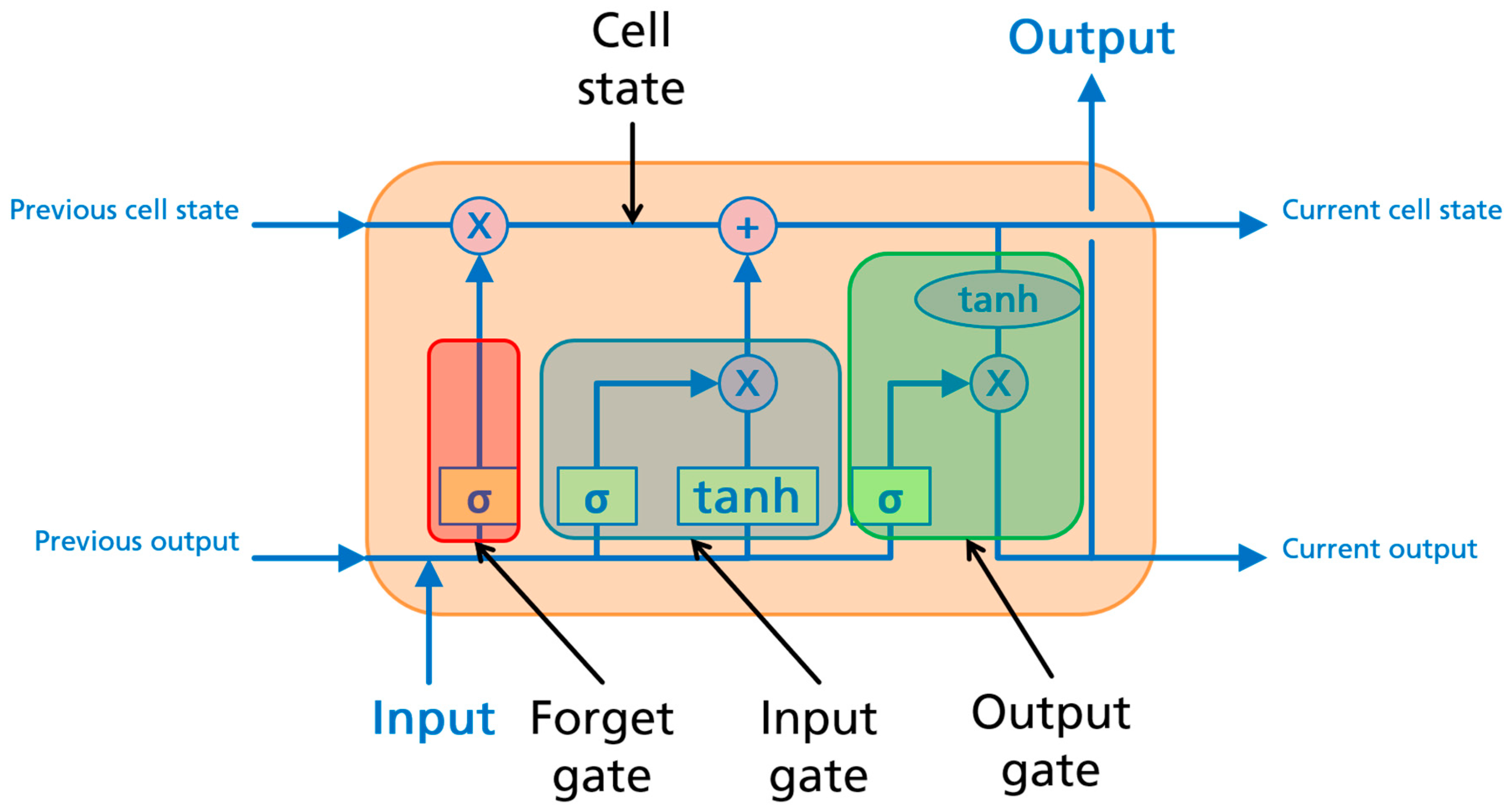
The Long Short-Term Memory architecture (Figure 1) consists of a memory cell that is connected by an input gate, an output gate and a forget gate. The forget gate ($f_t$) is the first gate in a LSTM unit and controls the information stored within the cell from the last time state ($c_{t-1}$) in accordance with Equation (2). The input gate determines which current information is used for the current state (Equation (3)), while the output gate controls the amount of information used for the output (Equation (4)):

$$f_t=\sigma \left(W_f·\left[h_{t-1},X_t\right]+b_f\right)$$

(2)

$$i_t=\sigma \left(W_i·\left[h_{t-1},X_t\right]+b_i\right)$$

(3)

$$o_t=\sigma \left(W_o·\left[h_{t-1},X_t\right]+b_i\right)$$

(4)

where a sigmoid activation function is denoted by $\sigma$, the different weights and biases by $W_x$ and $b_x$ of the candidate neuron, being the hidden layer output at time step t−1 and $X_t$ is the input vector at each time step.

The current hidden state of $c_t$ is determined by the following equations:

$${\tilde{c}}_t=tanh\left(W_c·\left[h_{t-1},X_t\right]+b_c\right)$$

(5)

$$c_t=f_t\ast c_{t-1}+i_t\ast {\tilde{c}}_t$$

(6)

where the hyperbolic tangent function ($tanh$) activation function is denoted by tanh, while $W_c$ and $b_c$ denote the weights and bias of the current gate. The output of an LSTM layer is calculated by the following equation:

$$h_t=o_t\ast tanh\left(c_t\right)$$

(7)

For further information, see Goodfellow et al. [37]. In this study, the LSTM implementation from Keras is used.

3.1.3. Standardized Load Profiles and Personalized Standard Load Profiles

In Germany, standardized load profiles were developed by the “Verband der Elektrizitätswirtschaft e. V.” (VDEW, Association of the Electricity Industry) using load measurements from 1209 different buildings [14]. In this study, it is used as a baseline benchmark to which the other methods are compared. Edwards et al., who compared commercial load profiles to residential load profiles, showed that commercial buildings have a significantly more stable load pattern than residential buildings [29]. Additionally with that, using fixed ruled algorithms based on statistics are a valuable option to load-forecasting in commercial buildings.

In total, there are 11 different profiles with a time resolution of 15 min. These are divided by the type of customer into: household (1 profile), commercial buildings (7 profiles) and agricultural companies (3 profiles). Every profile is further subdivided into nine different curves, with a differentiation between types of days (weekdays, Saturday and Sunday) and seasons (winter, summer and transition period;

Table 1. Seasonal separation for the standardized load profiles [14].

Season	Period
Summer	15/05–14/09
Transition	21/03–14/05 and 15/09–31/10
Winter	01/11–20/03

and Figure 2).

Public holidays within these periods are treated as Sundays because it is assumed that load patterns on these days are similar. Two exceptions for this rule are Christmas and New Year’s Day, which are treated as a Saturday if they do not fall on a Sunday. The load profiles are normalized to an annual consumption of 1000 kWh per annum and must be adapted to the specific annual consumption of the building under consideration. Forecasting is performed by applying the load profile values according to the season and time of day to the forecasting horizon [14].

As already described, several profile sets are available. Due to the characteristics of the load profiles in the observed commercial building, the G1 profile is chosen which is for commercial buildings with working hours of 8–18 on working days.

An extension of the standardized load profiles are the Personalized Standardized Load Profiles (PSLP). Like the SLP, the PSLP is a statistical model, with the advantage of not relying on predefined curves. The load profiles are derived from measured loads of the observed building. In contrast to the SLP, these are specific to the building and updatable in regular cycles when more recent measurements are available.

The preparation procedure for these profiles follow the methodology of the Standardized Load Profiles [6]: Initially, the measured loads are being classified into the same categories as the profiles of the SLP. Afterwards, the profiles are calculated using the mean value for every point of time in the three classes: weekday, Saturday and Sunday/holiday. In Figure 2, the process of calculating a weekday profile is exemplarily shown. The overlaid gray curves describe the historical measurements of one class and the red line describes the resulting averaged profile of the PSLP [7].

A general problem of the PSLP approach is that until a full year of load measurements is available, no profiles may be available for every season and day in the first year. To fill this gap, the profiles of the prior season are used in this study. Alike the standardized load profiles, forecasting is done by applying the different profiles according to the time of day, day type and season.

3.2. Data Exploration

The algorithms used in this study are data-driven approaches. Therefore, it is important to evaluate and understand the data first. Afterwards, the data must be explored to assess the quality of the datasets used and different features must be defined for use in the ML process.

In this study, two datasets of measured loads from different commercial buildings in Germany are used (

Table 2. Characteristics of the main and transferability datasets.

Dataset	MD	VD
Time period	1 December 2018–30 June 2019	2 March 2019–3 April 2019
Time resolution (after reduction)	5 min	5 min
Missing/Double data points (%)	0.2	3
Average load (kW)	19.89	3.12
Maximum load (kW)	84.74	10.43
Approx. annual load (MWh/a)	174.24	27.33

). The data is collected over a period of seven months (1 December 2018 to 30 June 2019) at a one second time resolution. One of the two datasets is used as the main dataset (MD), while the other is used as a validation dataset (VD) to validate the results. As the datasets do not include a complete year, the annual energy consumption had to be estimated. For this purpose, the average output in the measurement period was calculated and related to the entire year. For the optimization of the machine learning algorithms and the validation, the datasets were shortened to a period from 2 March 2019 to 3 April 2019 with all data prior being available for training. This period was chosen because of the absence of public vacations, making it an idealized dataset containing only working days and weekends.

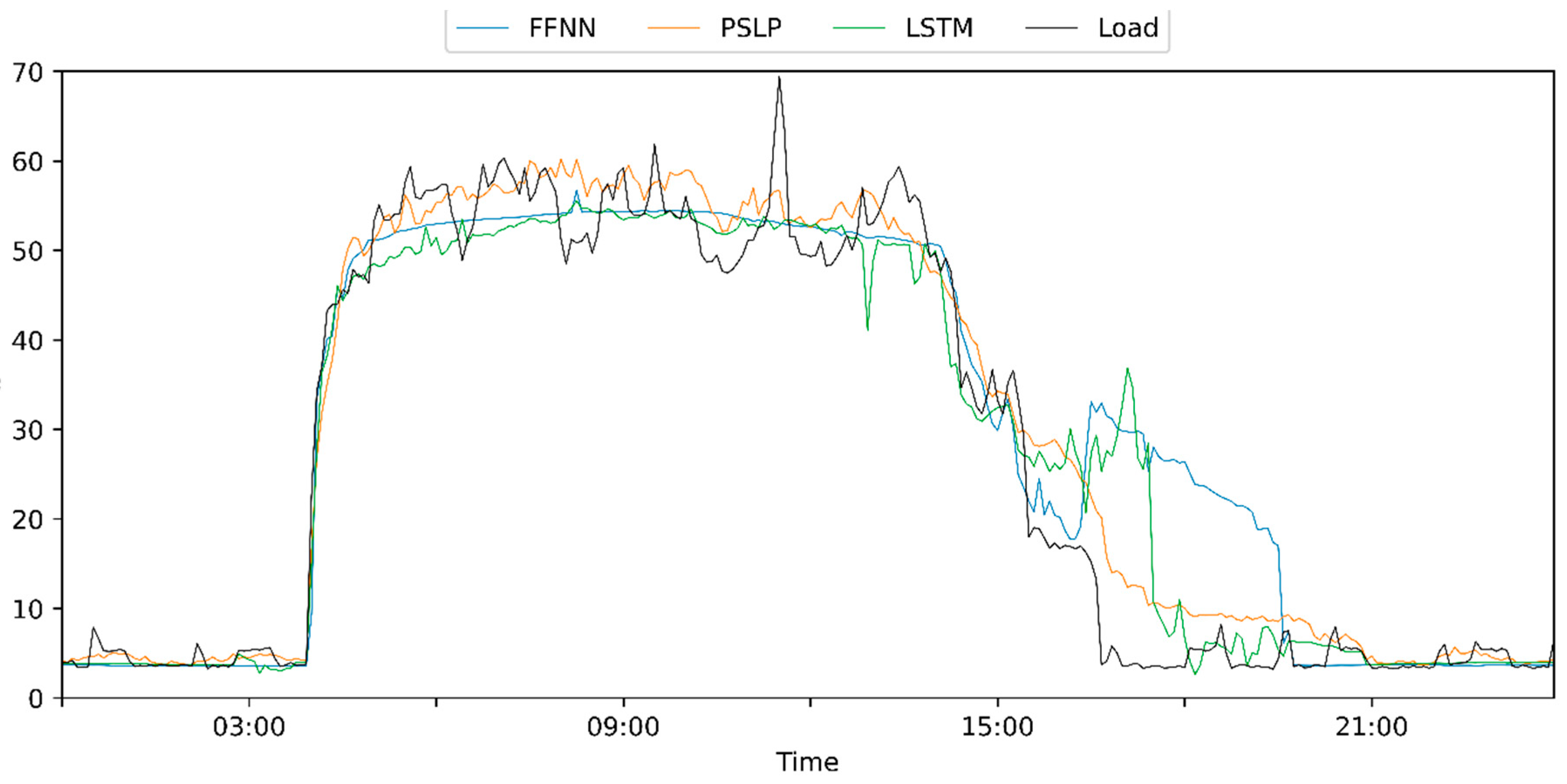
The load patterns in MD are constant throughout the measured period (Figure 3, upper), with around 50 kW on average and time-inconsistent peaks of up to 70 kW during working hours. The building base load is around 3.5 kW with peaks of up to 7 kW in non-working hours.

In the second commercial building (VD) (Figure 3, lower), on weekdays, the load pattern is nearly constant with a load profile of between 4 kW and 8 kW during working hours and peaks that exceed 10 kW. The weekends are inconsistent, with most having high and fluctuating loads, while on one weekend, base load was measured.

In comparison, the load profiles of the two datasets considerably differ. While loads are more constant in the MD, the loads in the VD building vary continually. The weekends are not as clear-cut for the VD building as for the MD building.

Data-driven methods for predictions heavily rely on the quality of data provided. Therefore, both datasets must be checked for inconsistencies such as missing or duplicate values. In the raw datasets of the MD, measurements are missed between 5 April 2019 and 8 April 2019, and between 12 April 2019 and 14 April 2019. That renders a total of 3% of the data missing in the MD and 0.2% in the VD.

3.3. Feature Description

Throughout the literature, many different features were introduced and many have proven to be valuable for load-forecasting as described in Section 2. The features (

Table 3. Selected features for load-forecasts done by ML algorithms.

Feature Group	Feature Name	Feature Description
Historical Features	Measurements of week before (W)	Measured loads at the exact same time the week before
	Measurements of day before (W)	Measured loads at the exact same time 24 h before
External features	Ambient air temperature (°C)	Actual ambient air temperature
Calendrical and timely features	Day indicator (1–7)	Day of the week by number
	Weekend indicator (0, 1)	Saturday/Sunday Monday–Friday
	Sine of week	Sine and cosine with one full cycle over a week
	Cosine of week
	Sine of day	Sine and cosine with one full cycle over a day
	Cosine of day
	Vacations (0, 1)	Indicator if day is a bank holiday

) used in this study are divided into three groups:

• Historical features;
• External features;
• Calendrical and timely features.

For historical features, two characteristics are used: the measured load of the previous week and of previous day at exactly the same time as the observed data point.

As an external feature, the temperature is used, which has been shown to have a large impact on the load and a good correlation with it [40]. As there is no data measured on site, datasets from the “Deutscher Wetterdienst” (DWD, German Meteorological Service) are used [41].

In the group of calendrical and timely features, six different factors are defined. The first is the day of the week, initiated by the numbers 1 to 7. The difference between weekdays and weekends, but also between weekdays and holidays, is represented by 0 and 1 and included as additional features. The last two characteristics used are the sine and cosine function, which have a complete cycle once a day or week, respectively, and introduce periodicity into the model.

3.4. Correlation Analysis

Ten features were selected as inputs for the ML algorithms. The correlation between the measured loads and selected features is calculated with the covariance $cov$ Equation (8). and the correlation $corr$ Equation (9) [42]:

$$cov\left(a,b\right)=\frac{1}{n-1}{\displaystyle \sum }_{i=1}^n(\left(a_i-\overline{a}\right)\times (b_i-\overline{b}))$$

(8)

$$corr\left(a,b\right)=\frac{cov\left(a,b\right)}{sd\left(a\right)\times sd\left(b\right)}$$

(9)

In Equation (8), $a$ and $b$ are the features and $\overline{a}$ and $\overline{b}$ as the means of the features. $sd$ describes the standard deviation of the respective features. To develop an in-depth understanding of the correlations, the data is evaluated once using the full dataset and one time using a monthly separated dataset, to find possible seasonal or calendrical relationships.

3.5. Evaluation Metrics

Different evaluation metrics have different meanings and benefits. The RMSE, has the benefit of penalizing large forecasting errors stronger than the MAE, because the error is squared for every data point on the forecasting horizon. To compare the different methods in more detail, four different metrics were used to evaluate the forecast accuracy. These are defined as:

$$MAE=\frac{1}{h}{\displaystyle \sum }_{t=n+1}^{n+h}\left|y_t^{\prime }-y_t\right|$$

(10)

$$MAPE=\frac{1}{h}{\displaystyle \sum }_{t=n+1}^{n+h}\left|\frac{y_t^{\prime }-y_t}{y_t^{\prime }}\right|$$

(11)

$$RMSE=\sqrt{\frac{1}{h}{\displaystyle \sum }_{t=n+1}^{n+h}{\left(\left|y_t^{\prime }-y_t\right|\right)}^2}$$

(12)

$$MASE=\frac{MAE}{\frac{1}{h-1}{{\displaystyle \sum }}_{t=n+1}^{n+h}\left|y_t-y_{t-7D}\right|}$$

(13)

In the formulas, $y_t^{\prime }$ is the predicted value and $y_t$ the measured one to a specific time step $n$ and number of time steps in the forecast horizon $h$. Whereas MAE, MAPE and RMSE are used in many studies (e.g., [11,12]), the MASE (Mean Absolute Scaled Error) is not often used and is further described in [13]. This metric differs from the other methods, as it is independent of the scale of the data. It compares the MAE reached by the tested method to a naive prediction that is, in this study, the seven-day previously measured power value ($y_{t-7D})$. With a value of the MASE below 1, the method performance used is better than the naïve forecast.

3.6. Load-Forecasting Tool Methodology

The concept of the developed load-forecast follows the idea of a constant data flow. The forecast algorithm should respond to changed behavior and provide updated, in-time load-forecasts, including the latest available measurements of the building. The methodology is shown in Figure 4 and described in the following sections. As datasets of varying length were used, an overview is given in Appendix A.

3.6.1. Online Sliding-Window Approach

In an operational environment, new data points are constantly collected. With every new data point, new information is available. Neural networks benefit from more and new information and therefore, the forecast accuracy can be improved.

In this study, this constant stream is simulated by a sliding window which is moved over the data. The forecast dataset (Figure 5) consists of the feature values in the time-period $t$ to the simulation time $t+forecasthorizon$. The training dataset always contains the example of the last n-data points within a time period from $t-window size$ to the simulation time $t$. All data prior to $t-window size$ is not used. After completion, the frame is shifted by one simulation step. This concept combines an offline training approach with a constant changing training dataset [43]. In literature, this is also referred to as online learning [44].

3.6.2. Data Pre-Processing

In the first step of the proposed sliding window methodology within the prediction process (Figure 4), the dataset must be pre-processed concerning the data quality, time resolution and preparation of an ML problem.

As quality issues were detected in the data exploration stage (Section 3.2) relating to missing data, these must be recovered first. The recovery of missing data points is achieved by linear interpolation. This methodology only works for reasonably small amounts of missing data.

As already mentioned in the Introduction, smart metering systems enable load measurements on building level with decreasing granularity. The incoming data is collected at a time resolution of 1 s and is subsequently transposed to a 5 min resolution. This is done to lower the amount of load peaks in the data while maintaining a low data granularity.

For the neural networks, the dataset is normalized by the “MinMaxScaler” provided with the python library Scikit-learn [45], which is based on Equation (14). In the formula, $x_{min}$ and $x_{max}$ are the lowest and highest values of the dataset. The data is normalized with $x_{scal}$ to the range between 0 and 1. Descriptive and target features are then normalized separately and the scalers $x_{scal}$ and $y_{scal}$ are cached. To avoid the introduction of new information, the scaler is refitted before each training step of the ML algorithms with the data used for the training of neural networks.

$$x_{scal}=\frac{x-x_{min}}{x_{max}-x_{min}}$$

(14)

3.6.3. Training and Forecasting

The training process (Figure 4) is limited to the length of the input data, or rather, the load measurements of the previous two months. The compiling of the neural networks is done once at the beginning of the sliding window forecast approach and then fitted to the given data. Afterwards, the neural networks always become refitted but not compiled again. The refitting process of the PSLP was performed every 24 h at 12 p.m. and, in contrast to the neural networks, implemented with all available data up to the current simulation time step.

As the ML algorithms use seven days of data as a descriptive feature (data from the previous week, Section 3.3), these data points are initially available for the PSLP. As the SLP is already fitted to the building using the annual consumption, no further training is conducted.

Forecasting is performed at every time step as an intra-day update.

3.6.4. Evaluation

For the evaluation (Figure 5), the predictions are first denormalized by using the cached scaler from the pre-processing stage (Section 3.6.2). Afterwards, the evaluation metrics described in Section 3.2 are used and cached across the entire simulation for every time step and saved at the end.

3.6.5. Algorithm Implementation and Optimization Procedure

Neural networks have many parameters that must be optimized in order to gain more accurate forecasts; a complete optimization will not be conducted in this study. The neural networks were designed using Keras [41] in Python 3.6 and optimized according to the number of layers and of neurons per layer (

Table 4. Optimization parameters for the ML algorithm network architectures.

Network Architectures
Number of Layers	1–8
Number of Neurons	8, 16, 32, 64, 128
Loss function	MAE
Optimizer	ADAM
Activation function	ReLU
Epochs	2000
Patience	50

). To prevent the training from being completed at a local minimum, but also to limit the process time, a patience factor is set at 50. The patience factor stops the iteration after the chosen number of 50 iterations if no better weight combinations were found and the best weights are restored.

The testing procedure is equivalent to the method described above but as mentioned in Section 3.2, has a shortened dataset containing the data of nearly two months (12 February 2019–4 April 2019).

The simulations were conducted on a server with 2 Intel Xeon E5-2630v4 with 2.20 GHz that have 10 Cores each and can handle 20 threads by using Hyper-Threading and 256 GB of ram.

3.7. Case Study: Integration of BEVs

In this section, details of the case study are described, demonstrating the integration of battery-electric vehicles (BEVs) into existing commercial buildings as an example for the use of load-forecasting-based energy management.

3.7.1. Case Study Description

The integration of BEVs into existing buildings is a challenging task. The overlap of the typically higher loads in a commercial building during working hours and the newly introduced high charging loads of the connected electric vehicles will require charging strategies to avoid overloading events. In this case study, 22 kW electric vehicle charging stations are virtually integrated into the MD building with its own smart meter. The charging stations are available as semi-public usable chargers that can be used by workers in the commercial building during the weeks and with no restrictions on the weekend. The goal of the system is to charge the electric vehicles as quickly as possible without compromising the buildings’ base loads within the grid connection limits. To achieve these objectives, charging is scheduled on the basis of the developed load-forecasts. For the simulation of the case study, six different scenarios are defined, with two, five and 10 charging stations integrated and using them with or without scheduled charging.

3.7.2. Charging Strategies

Several charging strategies are available for BEVs. This study focuses on uncontrolled charging and grid-oriented charging. In the uncontrolled charging strategy, the electric vehicles are always charged with the maximum possible power. In contrast, the grid-oriented charging strategy takes the load within the building grid into account so as to not exceed the grid limitations. This is achieved by lowering the charging load of the connected charging vehicles in light of the load-forecast for the next 24 h.

3.7.3. Simulation of Battery-Electric Vehicle Charging

Simulating the charging process of BEVs is simplified in this study by assuming a constant charging power that will be reduced if necessary. In this case study also, no seasonal effects on the batteries are considered and solely the power is observed. The charging schedule for the grid-oriented strategy is calculated using the load-forecast provided by the energy management system. In a first step, the free load capacity is calculated as the difference between the maximum grid connection capacity and the forecasted loads. The maximum grid connection capacity is set by the assumption that the maximum load measured equals 80%. For the MD, it is rounded to 110 kW. The free capacity is then split for every time step in the prediction between all vehicles according to their state of charge (SoC), the time connected to the charging station and the maximum charging load of the vehicle. With every prediction, the charging schedule is also updated.

3.7.4. Simulation of Battery-Electric Vehicle Charging

As no real-world data for the MD building was available, a synthetic dataset is generated for the simulation of arriving and departing times of BEVs.

Ten different profiles were randomly designed with the following parameters: different driven distances to work, different driving behavior on weekends and different arrival and departure times at the commercial building. To randomize the behavior of the drivers, an offset is randomly applied to each category “every day”. To fit these profiles to the building, the arriving time of the person to arrive earliest is set to the timestamp when building load increases. Analog to that, the last person scheduled to depart is set to the time when building consumption is around base load (Figure 3). In the time between these two timestamps, the other vehicles can arrive and leave randomly, but will usually stay around 8 h at the charging stations. Therefore, every charging station is used at least once every working day. The type of BEV is randomly assigned, with battery capacities between 18.7 kWh and 100 kWh and a charging power of 11 kW or 22 kW.

On the weekends, private citizens charge their cars at the stations. The chance of one person arriving at the building on the weekend between 8 a.m. and 10 p.m. is assumed to be 5%. In contrast to the profiles of the employees, the state of charge of the BEV is randomly calculated in the range of 5% to 20%.

The result of the presented process is shown as a heat map in Figure 6.

4. Results and Discussion

4.1. Feature Selection

The correlation between descriptive features and measured load can have seasonal dependencies. Figure 7 illustrates the correlation between descriptive features and the measured loads split in the month and for the entire dataset.

The correlation analysis demonstrates that the correlation between load measurements and descriptive features partially depends on seasonal effects. The features with the highest correlation directly derived from the dataset (Measurement of the week before, Measurement of the day before). The lower correlation of the Measurement of the day before is partly due to the fact that, for example, on a Saturday, the load values of Friday are used. Lower correlations are calculated for the independent sine and cosine features and the day and weekend indicators. In contrast to Cai et al. [40], the analysis shows fewer correlations between the temperature and load measurements with stronger monthly fluctuations. As the models derived by neural networks rely on the training data, fluctuations in the correlations can have an impact on the predictions. Therefore, updating neural network weights by refitting the network to new data is integrated into the workflow (Section 3.6.4, Figure 5). Additionally, described in Section 3.4, the Pearson coefficient is quantifying linear correlations. Higher degrees of correlations are therefore not investigated.

4.2. Initial Prediction Error

In contrast to the SLP, the PSLP and ML algorithms depend on the availability of load measurements from the building. As the ML algorithms rely on the feature, “Data of the last week”, these data are initially present for the PSLP. This leads to the PSLP being able to predict loads from the beginning of the simulation onwards in this study. The ML algorithms, in contrast, have an initial prediction error, as illustrated in Figure 8. The characteristics exhibit two periods of high forecasting errors within the first week of the simulation. The first peak is at the beginning of the simulation, as long as less data is available to derive a model (marker 1 and 2, lower graph, Figure 8). The second peak is reached when the first weekend occurs, as it is predicted by the network as a weekday (marker 3, Figure 8). This behavior must be considered when deploying a load-forecast-based load management system into the field. This is due to the high forecasting error of an untrained neural network on little data. The length of this event can vary but it is approximately about one combination of two working days and a weekend. With this procedure is a one-time event in the simulation; the assessment of activity in the following sections is adjusted evaluating the performance after the initial period.

4.3. Neural Network Architecture Optimization

Choosing a suitable architecture and parameters are an important step towards improving the forecast accuracy. A grid search was used to find optimal parameters by varying the number of layers from 1 to 10 and neurons from 8 to 128 neurons per layer. During optimization, a rolling forecast was used as well during a one-month period from 2 March 2019 to 3 April 2019 with all data prior to that period being available for training. An excerpt of the simulation results for different neural network architectures is shown in

Table 5. Excerpt of the optimization results. Forecast accuracy of different neural network architectures (averaged values of evaluation metrics).

	Configuration	MAE (W)	MASE	RMSE (W)
FFNN	1 Layer, 8 Neurons	3583	0.97	6198
	4 Layer, 8 Neurons	3508	0.92	6492
LSTM	2 Layer, 8 Neurons	3497	0.91	6197
	7 Layer, 8 Neurons	3426	0.88	6333

. The metrics (MASE, MAPE and RMSE) are listed, averaged over the test period.

The results demonstrate that both neural networks tend to perform worse with more neurons than the tested minimum number of eight neurons. Even an increase of hidden layers beyond four did not lead to a better performance, aside from the 7-layer and 8-neuron LSTM architecture. The MASE revealed that most neural network architectures with more layers and neurons are mostly worse than a persistency prediction. This also shows that although having stable load patterns, more sophisticated approaches like neural networks can improve forecast accuracy.

In total, there are several Feed-Forward Neural Network configurations with comparable results. The best results could be achieved with four layers and eight neurons each regarding the MASE and MAE, but worse for the RMSE compared to a network with one hidden layer and eight neurons. For this study, the more complex, with four hidden layers and eight neurons, was chosen because of its lower MAE and the much lower MASE compared to the one with 1 layer and 8 neurons.

For the LSTM, the 7-layer and 8-neuron architecture was chosen as for the FFNN, this architecture has the lowest MAE and MASE whereas the RMSE is slightly worse.

Comparing both of the selected neural network architectures, the LSTM outperforms the FFNN by having higher forecast accuracies on all scales. In the next section, the neural network architectures are used on a longer dataset containing vacations and it is assessed how they perform against the SLP and PSLP as their benchmarks.

4.4. Comparison of Load-Forecasting Methods

The previously optimized ML algorithms are used to evaluate the real performance on the full main dataset. This includes public vacations and different seasons. The averaged results are shown in

Table 6. Comparison of the algorithm performance on the whole MD (averaged values of evaluation metrics).

	MAE (kW)	RMSE (kW)	MAPE (%)
FFNN	4.11	8.35	50.34
LSTM	4.47	9.29	51.42
PSLP	3.99	9.09	53.22
SLP	9.26	16.65	69.4

and median results in

Table 7. Comparison of the algorithm performance on the whole MD (median values of evaluation metrics).

	MAE (kW)	RMSE (kW)	MAPE (%)
FFNN	3.39	5.15	26.53
LSTM	3.68	5.54	28.96
PSLP	3.31	5.26	27.47
SLP	10.79	17.61	41.28

.

In comparison to the SLP, the data-based algorithms perform significantly better than the SLP. The FFNN performs best on the MAPE and RMSE evaluation metrics, but is outperformed by the PSLP on the MAE. Within the optimization stage, the LSTM performs worse than the FFNN and is also outperformed by the PSLP. The averaged MAEs are within a range of around 4.7% to 5.3% of the peak load for the data-driven algorithms, which is compared to the 11% for the SLP which measured a significant improvement.

In comparison between the averaged values and the median values, the metrics differ significantly because of days with untypical patterns being predicted with high forecasting errors (e.g., days between holidays and weekends are mostly predicted as a weekday, but have a weekend pattern).

Figure 9 presents the boxplots of the forecasting errors to have a deeper view on the error distribution. A boxplot consists of a box, or the so-called interquartile range, the whiskers (upper and lower lines), the median (orange line) and usually outliers, which are not shown in the figure. The interquartile range contains 50% of all the values. Value errors higher or lower than the interquartile range are described by the whiskers. All other data points are considered outliers. The boxplots show that the SLP has the largest error distributions in all three metrics with a large interquartile range and a high distance between the box and the upper whisker.

The boxes show the interquartile range which contains 50% of the values whereas values higher or lower are described by the whiskers. The orange line indicates the median.

Significant for all of the three methods is the high number of outliers present beyond the upper whiskers (maxing out at: MAE 34 kW, RMSE: 205 kW, MAPE: 870% on public holidays). The ML approaches slightly outperform the PSLP on the MAE and RMSE scale by having a smaller interquartile range, a comparable or lower upper whisker and lower median (orange lines). This shows that both can predict the future loads more consistently and more accurately as the PSLP. In contrast to the MAE, FFNN and PSLP performing similar on the MAPE metric, the LSTM has a higher lower whisker and a lower interquartile range while maintaining a lower upper whisker.

As mentioned in Section 4.2, there is an initial prediction error of the ML algorithms in the first week. In total, the differentiation between predictions on weekdays and weekends is clearly outlined by the height of the prediction error. On weekends, the MAE is typically lower than the MAE on weekdays due to the lower and less fluctuating loads.

To further evaluate the behavior, a closer look is taken into the prediction of a weekday (Figure 10). In contrast to the increase of the load demand in the morning (4 a.m.), which has a higher degree of regularity, smaller load peaks and the decrease in the load cannot be predicted so accurately (5 p.m.). It is also shown that compared to the PSLP (orange), both neural networks (FFNN: blue; LSTM: green) tended to predict constant loads during working hours.

4.5. Adaptability of the ML Algorithms/Public Holidays

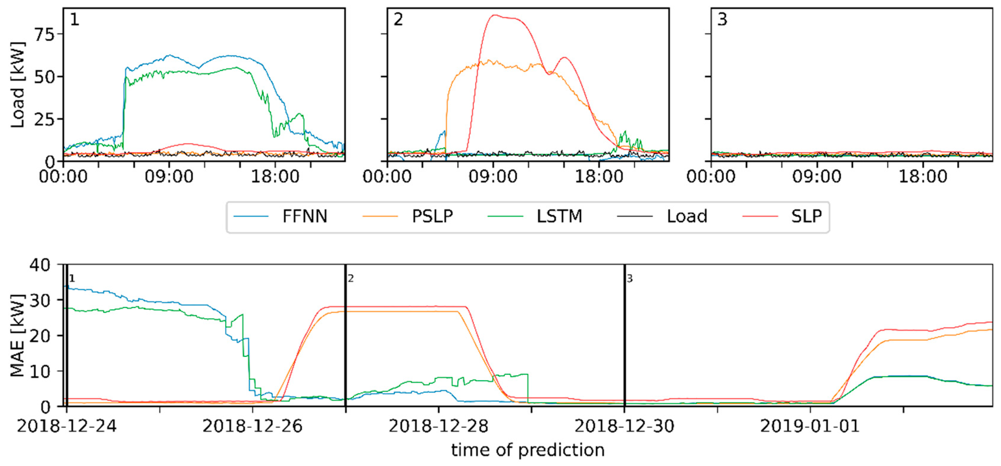
Adapting new patterns must be performed automatically by the load-forecasting algorithm in order to provide accurate forecasts and to be as self-maintaining as possible. This is evaluated by using the Christmas holidays as an example of an abrupt change in user load demand behavior in the building.

Regarding Figure 11, the ML algorithms automatically adapt the new behavior. The adaptation process for both algorithms has three steps. The first step is characterized by a high prediction error (Figure 11, marker 1). The adaptation stage (step 2), which can lead to an abrupt decrease such as in the case of the FFNN or has an increased MAE (LSTM) again. In the last stage, the adaptation is completed (Figure 11, marker 3) until the next public holiday on the 1st of January.

In contrast to that, the PSLP and SLP follow fixed rules, described in Section 3.1.3, and do not adopt the new patterns automatically. Both have a high forecasting error, because the prediction on 27 December was categorized as a working day (Figure 11, marker 2). This is a problem when using methods with fixed rules because they must be monitored manually or new and personalized rules have to be implemented so that they can react to unforeseen changes.

In contrast to the neural networks, events like public vacations can be accurately predicted by the PSLP and SLP if they are specified. The ML algorithms can predict vacations as well, but as they are a data-driven approach, they require examples in the dataset (Figure 12). As the training dataset does not include vacations, the prediction error arises when the first vacation date occurs (Figure 12, marker 1). When the new situation arises, the FFNN predict even negative values, although no negative values are available in the dataset. Unlike the LSTM, the prediction on the second public vacation some weeks later, the FFNN predicts the load demand more accurately, whereas the LSTM still predicts high loads (Figure 12, marker 2).

4.6. Validation of Load-Forecasting Results

Optimizing neural networks for new buildings is time consuming and requires long time-series of measured loads from the new buildings. Therefore, in this section, non-pre-trained neural networks are used on the validation dataset (VD) which have the same architecture like the ones used for the MD in the previous sections. A comparison of the results is illustrated in Figure 13.

The MAPE reveals that the PSLP (orange) performs slightly better on the MD than on the VD while the ML algorithms (LSTM: green; FFNN: blue) perform better on the VD. The same is shown by the MASE in case of changing load patterns; the persistency forecast accuracy is decreased and therefore, the MASE also decreased for all algorithms.

As is shown in Section 4.2, the initial prediction error also appears, when predicting on the basis of the VD dataset (Figure 14). It was pointed out in Section 3.2 that the loads on the weekends differ significantly between the MD and VD. This can also be observed in the MAE profile, with the weekends not as visible in the VD as the MD. It is demonstrated that the behavior of the algorithms used is comparable in both datasets, with a slight exception in the PSLP. This algorithm sometimes has a significantly higher or lower MAE compared to the ML algorithms on the VD, while the MAE of all algorithms is more equal on the MD.

Due to the differences in the results regarding the MASE and MAPE, it is better to optimize the neural network architecture once again for the VD. Therefore, using ML-approaches for load management applications is more complex than using simple PSLP. But the potentials of having even higher forecasting accuracies with more sophisticated algorithms are important to accurately manage loads in a self-maintaining environment. The ability to use the same neural network architecture for different datasets/buildings can be a key factor for fast deployment, as well as the use of pre-trained algorithms. This would lower the complexity of the problem deploying a load-forecast-based energy management system, so that it is usable without having measurements over a long time period and to avoid individual optimization work.

4.7. Results Case Study

The scenarios described in Section 4 were simulated using the shortened MD. The FFNN is used as a forecast algorithm.

According to

Table 8. Results of the simulations of the integration of electric vehicles by using load-forecasts to control charging.

Number of Charging Stations	2		5		10
Scenario	Controlled	Uncontrolled	Controlled	Uncontrolled	Controlled	Uncontrolled
Average energy charged (kWh)	24.75	24.75	23.41	23.41	23.84	23.84
Average charging duration (hours)	01:26:02	01:26:02	01:36:09	01:32:37	02:10:17	01:32:22
Registered overloads	0	0	7	90	605	826
Maximum Overload (kW)	0	0	9.7	24.9	20.24	65.15
Mean overload (kW)	0	0	3.38	6.86	3.91	23.89

, the integration of two charging stations did not show any problem, as no overload was registered and the system did not influence the charging procedure. This changes for the scenario with five charging stations, as the average charging duration increased by about four minutes. The calculated mean and maximum overload-for the controlled charging reflect how high the overload of the grid connection would be if the energy management system were to charge as scheduled. Due to the scheduled charging, both significantly decreased. This is also shown in the simulated scenario with 10 charging stations. As a result of the larger number of vehicles and the limited available capacity for all vehicles, the averaged charging duration increases by over 30 min.

To further evaluate the issue, Figure 15 points out that if the load prediction over-estimates the loads, the scheduled charging loads will be significantly lower and therefore, will not charge at the limit and so will not exceed it. For underestimation, which is shown in Table 8 by the registered overloads, the opposite occurs. The initial prediction error which was researched for the neural networks is also applicable to the PSLP, as with no data available, no predictions can be done and the system cannot manage the loads.

Another issue arises regarding the change of behavior within the building when, for example, tenants change. In Section 4.4 and Section 4.6, with regards to the load pattern characteristics described in Section 3.2 of adopting new patterns. In contrast to that, statistical approaches need new rules to be able to (see Section 4.5). In both cases, the changes were not significant. A more significant change could be in a multi-customer commercial building, when one tenant with high loads or several tenants move out. This can lead to significant changes and can result in high forecasting errors which will be reduced automatically by the ML approaches. For the PSLP, a reset of the load profiles might be needed to adapt major changes in the load behavior. Anyway, both methods lead to potentially unavoidable high forecasting errors which affects the scheduling of dynamic loads. High forecasting errors on public holidays are unavoidable, too, but as commercial buildings tend to have low loads on these days, the problem slightly distinguishes compared to high forecast errors on weekdays. The initial prediction error must always consider if ML techniques were chosen.

All of that leads to the fact that load-forecasting approaches can be used to estimate charging schedules for BEV. However, the aforementioned characteristics also show that the different used approaches have different benefits and shortcomings for load management applications.

Additionally, a load-forecast-based energy system can provide the electric vehicle’s owner with information if charging the vehicle is possible and also gives the owner of the charging station new opportunities for private-public charging stations without compromising the base load of its building and the implementation of new tariff systems.

5. Conclusions and Outlook

Many studies in recent years have proven that machine learning techniques are capable of predicting loads. In this study, the performance of traditional load-forecasting methods, namely SLP and PSLP, and basic neural networks, LSTM and FFNN, was investigated for energy management applications. The results show that the SLP is not capable of forecasting loads because of high forecasting errors. This is due to the fact that these profiles were not derived using on-site measured data. By transferring the methodology of the SLP to on-site measured data (PSLP), the performance improved significantly.

For energy management applications, changes are highly problematic, as these must be adopted by the algorithms as fast as possible to ensure low forecasting errors and therefore, accurate predictions. Due to fixed rules, the PSLP cannot adapt to these changes (Section 4.5) as fast as neural networks can. This could be changed by implementing more rules or even shortening the lookback for profile calculation. Then, this approach could be a reasonable consideration as a simple approach to load-forecasting for single commercial buildings (Section 4.4).

In Section 4.6, the used algorithms were tested on a second dataset without another hyperparameter optimization step for the neural networks. This was done to examine if comparable results are expectable. The results showed that further optimization would be needed, which makes the implementation of neural networks into an energy management system an additional step to further increase forecasting performance.

As a use case, the usage of load-forecasting in the energy management system of an existing commercial building to integrate BEV charging infrastructure was designed and simulated. Especially for energy management applications, low granularities of the data are beneficial because of the overall fluctuation of the loads compared to higher granularities. This ensures more accurate scheduling and also the ability to predict load peaks. The results indicate that the lower the forecasting error is, the smaller the maintained capacity can be, and concerning the presented case, the more charging stations can be integrated.

Generally, by using a load-forecasting-based energy management system, there can be a significant decrease in height and amounts of overloads. However, due to the aforementioned forecast errors, it is still important that the energy management system always measures and limits the loads in a timely manner, as the load-forecast can only provide a rough estimate of how high the loads will be. In summary, load-forecasting can be used to shift loads or, at least, provide information when these consumers can be used to not compromise the base loads of the building. This allows for an expectation management of the customers, informing them early about charging schedules and their changes. Additionally, in combination with a PV power prediction, the self-consumption can be increased and therefore, the loads of grid connection become relieved. As already mentioned, although there are several benefits of using ML algorithms for load-forecasting, statistical methods are still very capable for that as well. Nevertheless, the full potential of ML algorithms must be further evaluated and more sophisticated neural network architectures have to be applied to the problem of single building level forecasting. As discussed in the validation optimizing, neural networks to new buildings could lead to better forecasts but this has to be evaluated in further studies. By combining statistical and ML approaches, a reliable load management system could be introduced to the problem. As an example, the PSLP could support the ML algorithm by bridging the gap between the first measurements until accurate predictions are available and during public vacations. It is also possible to use the PSLP as a feature for training of neural networks as these have proven to be valuable to forecast loads in a commercial building. Moreover, the PSLP could bridge times between training of neural networks if it is not finished in time or problems arise, such as false forecasts or other issues. In total, the energy management system must still decide and regulate loads in time in order to ensure maximum charging power to every point in time and prevent overloads.

Related to the framework, the algorithms must be tested in an operational energy management system environment to further evaluate the problems arising by using ML algorithms and PSLP for load-forecasting. This also applies to the use case of integrating electric vehicles into an existing building, as many assumptions had to be made.

Neural network optimization was constrained for two different layers (dense and LSTM) and a fixed number of neurons per layer. In future work, more parameters, such as activation function, dropout or number of epochs, can be included in the hyperparameter optimization. The use of a different hyperparameter optimization as offered by Optuna [46] could improve the prediction model. Feature selection was simplified by using linear correlation coefficients, which cannot describe higher degrees of dependencies. By using other methods, such as decision tree-based methods, the selected features may differ and further increase the prediction accuracy. Furthermore, the results of the study were validated on a small dataset. Therefore, the results should be further investigated and validated by using multiple years of data and also by utilizing load measurements of other building types.

The case study is limited by the assumption that the BEV load can be measured separately, which is not possible in every building or only by an additional cost-intensive measurement. Therefore, predicting the combined load of BEV and building base load can be an important and challenging task. Moreover, the combination with local generation such as a PV system may require a combined forecast of generation and load [47].

Uncertainty quantification will also become necessary for the robust application of a forecasting model in load management. A first step could be probabilistic forecasts, such as described by Kong et al. [48].

In future research, the focus should also be taken onto the change of the needed neural network architecture. As an option to implement hyperparameter optimization in an operational environment, cloud services could be a key factor. Or even going further, the whole training can be done in the cloud with the trained model used locally for forecasting.

As is demonstrated by the used case, load-forecasts can support energy management systems. The forecast-based operational strategies of flexible consumers and battery storage capacities must be researched. Concerning the integration of the three main sectors, the integration of electrical space heaters or heat pumps is also made possible by combining the forecasts of heat usage and load-forecasting.