
Enhanced Random Forest Model for Robust Short-Term Photovoltaic Power Forecasting Using Weather Measurements

 ,
, 
 and
and
Abstract
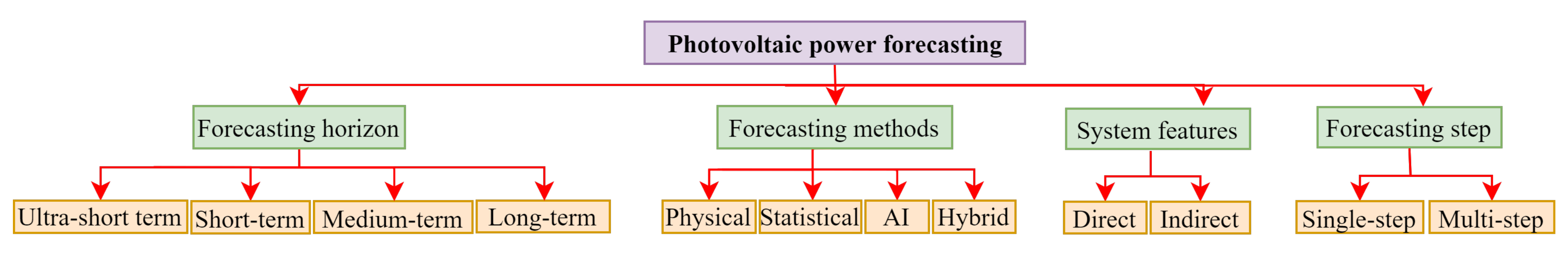
:1. Introduction
- 1.
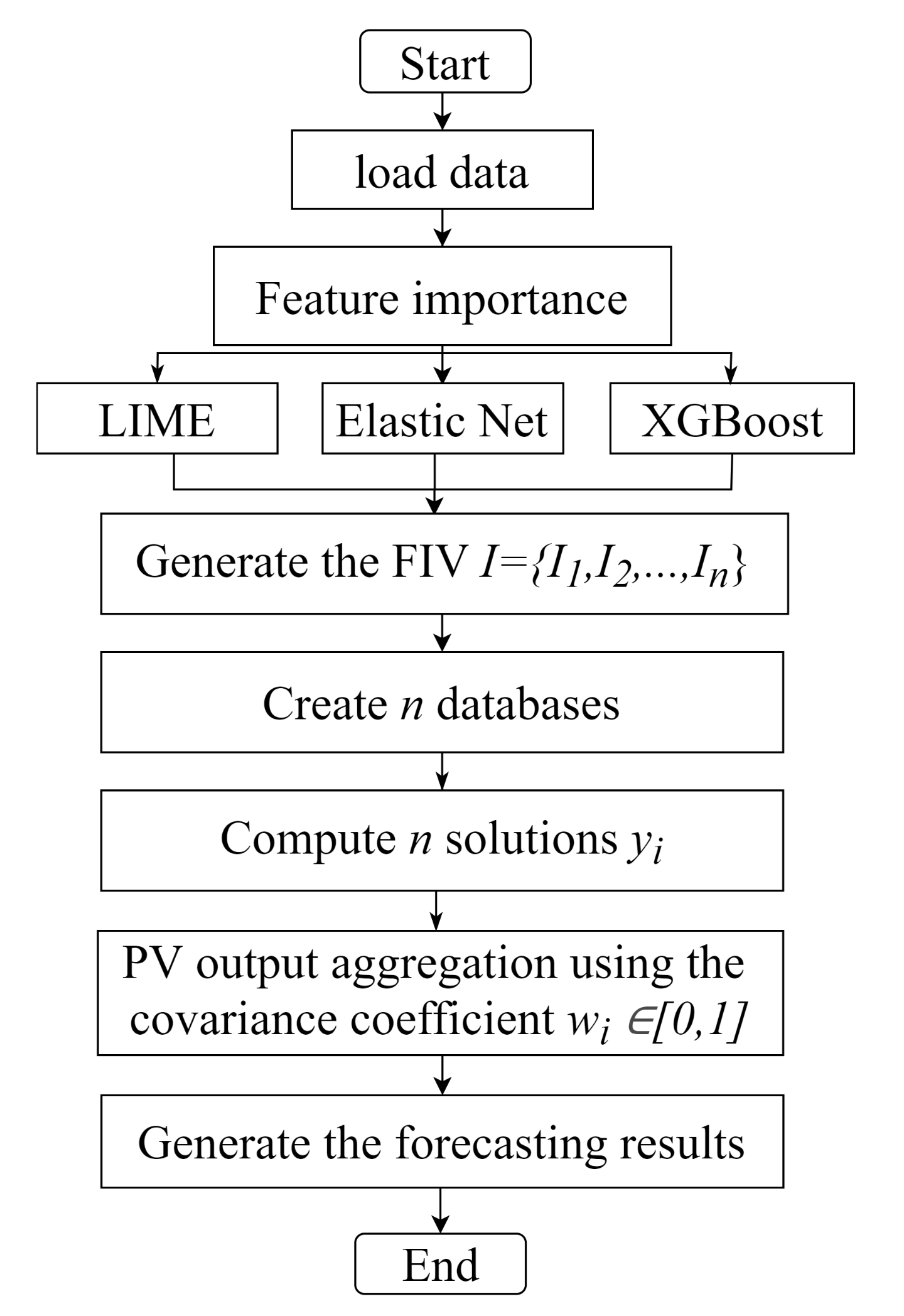
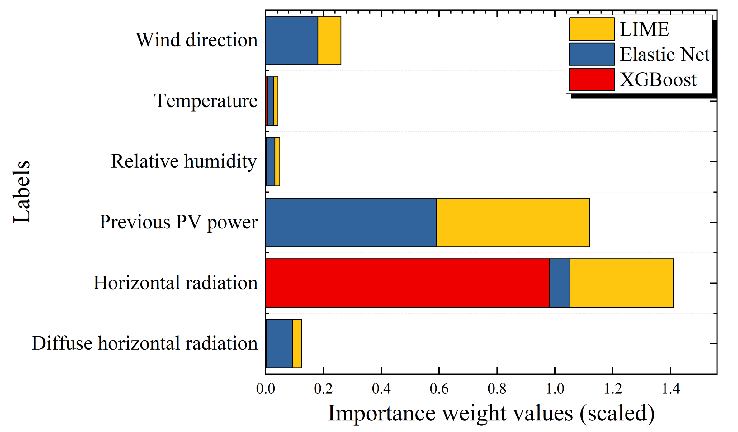
- An effective feature engineering technique is deployed based on six input parameters using three different approaches. The features are classified according to their weights. FVI is calculated using the input parameters relevant to the PPF model.
- 2.
- A new approach-based-multimodal prediction system is comprehensively investigated.
- 3.
- The performance superiority of the proposed approach versus Decision Trees (DT), K-Nearest Neighbors (KNN), and Random decision forest (RF) is demonstrated using a real data set.
2. Literature Review
3. Problem Statement and Contributions
4. Proposed Methodology
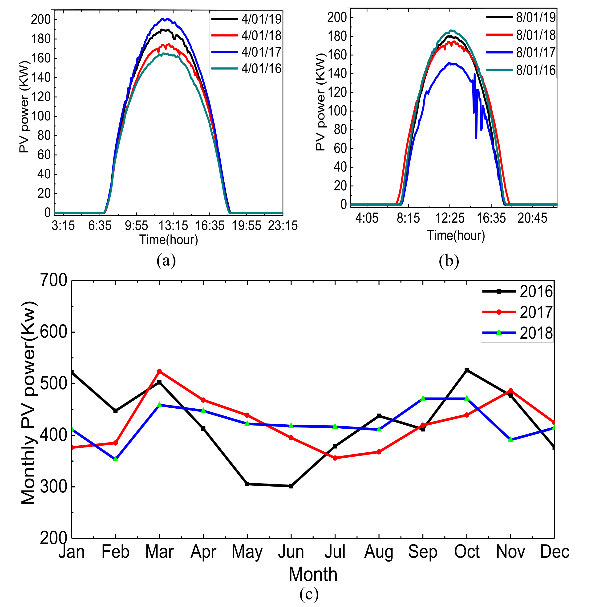
5. Case Study
5.1. PV System Description
5.2. Feature Engineering
5.3. Feature Vector Construction
5.4. Simulation Results and Comparison with Benchmark Models
5.5. Discussion and Analysis
6. Conclusions
Author Contributions
Funding
Data Availability Statement
Conflicts of Interest
Abbreviations
| SE | Solar Energy |
| LSSVR | Least squares support vector regression |
| MAD | Mean Absolute Deviation |
| RMSE | Root Mean Square Error |
| NMAE | Normalized Mean Square Error |
| WMAE | Weighted Mean Square Error |
| Coefficient of determination | |
| MAPE | Mean Absolute Percent Error |
| CNN | Convolutional Neural Network |
| MRE | Mean Relative Error |
| RNN | Recurrent Neural Network |
| NARX | Non linear Auto-Regressive with Exogenous inputs |
| ARMAX | Autoregressive-Moving-Average model with Exogenous inputs |
| SD | Standard Derivation |
| ARMA | Autoregressive-Moving-Average |
References
- Rajagukguk, R.A.; Ramadhan, R.A.; Lee, H.J. A Review on Deep Learning Models for Forecasting Time Series Data of Solar Irradiance and Photovoltaic Power. Energies 2020, 13, 6623. [Google Scholar] [CrossRef]
- Zervos, A.; Lins, C.; Muth, J. RE-Thinking 2050: A 100% Renewable Energy Vision for the European Union; Erec: Brussels, Belgium, 2010. [Google Scholar]
- Akhter, M.N.; Mekhilef, S.; Mokhlis, H.; Shah, N.M. Review on forecasting of photovoltaic power generation based on machine learning and metaheuristic techniques. IET Renew. Power Gener. 2019, 13, 1009–1023. [Google Scholar] [CrossRef] [Green Version]
- Massaoudi, M.; Refaat, S.S.; Abu-Rub, H.; Chihi, I.; Oueslati, F.S. PLS-CNN-BiLSTM: An End-to-End Algorithm-Based Savitzky–Golay Smoothing and Evolution Strategy for Load Forecasting. Energies 2020, 13, 5464. [Google Scholar] [CrossRef]
- Salamanis, A.I.; Xanthopoulou, G.; Bezas, N.; Timplalexis, C.; Bintoudi, A.D.; Zyglakis, L.; Tsolakis, A.C.; Ioannidis, D.; Kehagias, D.; Tzovaras, D. Benchmark Comparison of Analytical, Data-Based and Hybrid Models for Multi-Step Short-Term Photovoltaic Power Generation Forecasting. Energies 2020, 13, 5978. [Google Scholar] [CrossRef]
- Alam, A.M.; Razee, I.A.; Zunaed, M. Solar PV Power Forecasting Using Traditional Methods and Machine Learning Techniques. In Proceedings of the 2021 IEEE Kansas Power and Energy Conference (KPEC), Manhattan, KS, USA, 19–20 April 2021; IEEE: New York, NY, USA, 2021; pp. 1–5. [Google Scholar]
- Dong, Z.; Yang, D.; Reindl, T.; Walsh, W.M. Short-term solar irradiance forecasting using exponential smoothing state space model. Energy 2013, 55, 1104–1113. [Google Scholar] [CrossRef]
- Li, Y.; Su, Y.; Shu, L. An ARMAX model for forecasting the power output of a grid connected photovoltaic system. Renew. Energy 2014, 66, 78–89. [Google Scholar] [CrossRef]
- Işığıçok, E.; Öz, R.; Tarkun, S. Forecasting and Technical Comparison of Inflation in Turkey With Box-Jenkins (ARIMA) Models and the Artificial Neural Network. Int. J. Energy Optim. Eng. (IJEOE) 2020, 9, 84–103. [Google Scholar] [CrossRef]
- Van der Meer, D.; Mouli, G.R.C.; Mouli, G.M.E.; Elizondo, L.R.; Bauer, P. Energy management system with PV power forecast to optimally charge EVs at the workplace. IEEE Trans. Ind. Inform. 2016, 14, 311–320. [Google Scholar] [CrossRef] [Green Version]
- Ding, M.; Wang, L.; Bi, R. An ANN-based approach for forecasting the power output of photovoltaic system. Procedia Environ. Sci. 2011, 11, 1308–1315. [Google Scholar] [CrossRef] [Green Version]
- Karabacak, K.; Cetin, N. Artificial neural networks for controlling wind–PV power systems: A review. Renew. Sustain. Energy Rev. 2014, 29, 804–827. [Google Scholar] [CrossRef]
- Al-Dahidi, S.; Ayadi, O.; Adeeb, J.; Louzazni, M. Assessment of artificial neural networks learning algorithms and training datasets for solar photovoltaic power production prediction. Front. Energy Res. 2019, 7, 130. [Google Scholar] [CrossRef] [Green Version]
- Cervone, G.; Clemente-Harding, L.; Alessandrini, S.; Delle Monache, L. Short-term photovoltaic power forecasting using Artificial Neural Networks and an Analog Ensemble. Renew. Energy 2017, 108, 274–286. [Google Scholar] [CrossRef] [Green Version]
- Shah, A.A.; Ahmed, K.; Han, X.; Saleem, A. A Novel Prediction Error Based Power Forecasting Scheme for Real PV System using PVUSA Model: A Grey Box Based Neural Network Approach. IEEE Access 2021. [Google Scholar] [CrossRef]
- Almonacid, F.; Pérez-Higueras, P.; Fernández, E.F.; Hontoria, L. A methodology based on dynamic artificial neural network for short-term forecasting of the power output of a PV generator. Energy Convers. Manag. 2014, 85, 389–398. [Google Scholar] [CrossRef]
- Chen, C.; Duan, S.; Cai, T.; Liu, B. Online 24-h solar power forecasting based on weather type classification using artificial neural network. Sol. Energy 2011, 85, 2856–2870. [Google Scholar] [CrossRef]
- Raza, M.Q.; Nadarajah, M.; Ekanayake, C. A multivariate ensemble framework for short term solar photovoltaic output power forecast. In Proceedings of the 2017 IEEE Power & Energy Society General Meeting, Chicago, IL, USA, 6–20 July 2017; IEEE: New York, NY, USA, 2017; pp. 1–5. [Google Scholar]
- Al-Dahidi, S.; Ayadi, O.; Alrbai, M.; Adeeb, J. Ensemble approach of optimized artificial neural networks for solar photovoltaic power prediction. IEEE Access 2019, 7, 81741–81758. [Google Scholar] [CrossRef]
- Chai, Z.; Zhao, C. Enhanced random forest with concurrent analysis of static and dynamic nodes for industrial fault classification. IEEE Trans. Ind. Inform. 2019, 16, 54–66. [Google Scholar] [CrossRef]
- Mellit, A.; Massi Pavan, A.; Ogliari, E.; Leva, S.; Lughi, V. Advanced methods for photovoltaic output power forecasting: A review. Appl. Sci. 2020, 10, 487. [Google Scholar] [CrossRef] [Green Version]
- Massucco, S.; Mosaico, G.; Saviozzi, M.; Silvestro, F. A hybrid technique for day-ahead PV generation forecasting using clear-sky models or ensemble of artificial neural networks according to a decision tree approach. Energies 2019, 12, 1298. [Google Scholar] [CrossRef] [Green Version]
- Ogliari, E.; Dolara, A.; Manzolini, G.; Leva, S. Physical and hybrid methods comparison for the day ahead PV output power forecast. Renew. Energy 2017, 113, 11–21. [Google Scholar] [CrossRef]
- Massaoudi, M.; Chihi, I.; Sidhom, L.; Trabelsi, M.; Refaat, S.S.; Abu-Rub, H.; Oueslati, F.S. An effective hybrid NARX-LSTM model for point and interval PV power forecasting. IEEE Access 2021, 9, 36571–36588. [Google Scholar] [CrossRef]
- Massaoudi, M.; Abu-Rub, H.; Refaat, S.S.; Chihi, I.; Oueslati, F.S. Deep Learning in Smart Grid Technology: A Review of Recent Advancements and Future Prospects. IEEE Access 2021, 9, 54558–54578. [Google Scholar] [CrossRef]
- Gigoni, L.; Betti, A.; Crisostomi, E.; Franco, A.; Tucci, M.; Bizzarri, F.; Mucci, D. Day-ahead hourly forecasting of power generation from photovoltaic plants. IEEE Trans. Sustain. Energy 2017, 9, 831–842. [Google Scholar] [CrossRef] [Green Version]
- Abdel-Nasser, M.; Mahmoud, K. Accurate photovoltaic power forecasting models using deep LSTM-RNN. Neural Comput. Appl. 2019, 31, 2727–2740. [Google Scholar] [CrossRef]
- Yang, M.; Huang, X. Ultra-short-term prediction of photovoltaic power based on periodic extraction of PV energy and LSH algorithm. IEEE Access 2018, 6, 51200–51205. [Google Scholar] [CrossRef]
- Graupe, D.; Krause, D.; Moore, J. Identification of autoregressive moving-average parameters of time series. IEEE Trans. Autom. Control 1975, 20, 104–107. [Google Scholar] [CrossRef]
- Da Costa Lopes, F.; Watanabe, E.H.; Rolim, L.G.B. A control-oriented model of a PEM fuel cell stack based on NARX and NOE neural networks. IEEE Trans. Ind. Electron. 2015, 62, 5155–5163. [Google Scholar] [CrossRef]
- Li, G.; Xie, S.; Wang, B.; Xin, J.; Li, Y.; Du, S. Photovoltaic Power Forecasting With a Hybrid Deep Learning Approach. IEEE Access 2020, 8, 175871–175880. [Google Scholar] [CrossRef]
- Tao, C.; Shanxu, D.; Changsong, C. Forecasting power output for grid-connected photovoltaic power system without using solar radiation measurement. In Proceedings of the 2nd International Symposium on Power Electronics for Distributed Generation Systems, Hefei, China, 16–18 June 2010; IEEE: New York, NY, USA, 2010; pp. 773–777. [Google Scholar]
- Massaoudi, M.; Abu-Rub, H.; Refaat, S.S.; Chihi, I.; Oueslati, F.S. An Effective Ensemble Learning approach-Based Grid Stability Assessment and Classification. In Proceedings of the 2021 IEEE Kansas Power and Energy Conference (KPEC), Manhattan, KS, USA, 19–20 April 2021; IEEE: New York, NY, USA, 2021; pp. 1–6. [Google Scholar]
- Razagui, A.; Abdeladim, K.; Semaoui, S.; Arab, A.H.; Boulahchiche, S. Modeling the forecasted power of a photovoltaic generator using numerical weather prediction and radiative transfer models coupled with a behavioral electrical model. Energy Rep. 2020, 6, 57–62. [Google Scholar] [CrossRef]
- Diagne, M.; David, M.; Lauret, P.; Boland, J.; Schmutz, N. Review of solar irradiance forecasting methods and a proposition for small-scale insular grids. Renew. Sustain. Energy Rev. 2013, 27, 65–76. [Google Scholar] [CrossRef] [Green Version]
- Massaoudi, M.; Abu-Rub, H.; Refaat, S.S.; Chihi, I.; Oueslati, F.S. Accurate Smart-Grid Stability Forecasting Based on Deep Learning: Point and Interval Estimation Method. In Proceedings of the 2021 IEEE Kansas Power and Energy Conference (KPEC), Manhattan, KS, USA, 19–20 April 2021; IEEE: New York, NY, USA, 2021; pp. 1–6. [Google Scholar]
- Sansa, I.; Missaoui, S.; Boussada, Z.; Bellaaj, N.M.; Ahmed, E.M.; Orabi, M. PV power forecasting using different artificial neural networks strategies. In Proceedings of the 2014 First International Conference on Green Energy ICGE 2014, Sfax, Tunisia, 25–27 March 2014; IEEE: New York, NY, USA, 2014; pp. 54–59. [Google Scholar]
- Mohanty, S.; Patra, P.K.; Sahoo, S.S.; Mohanty, A. Forecasting of solar energy with application for a growing economy like India: Survey and implication. Renew. Sustain. Energy Rev. 2017, 78, 539–553. [Google Scholar] [CrossRef]
- Lobaccaro, G.; Carlucci, S.; Löfström, E. A review of systems and technologies for smart homes and smart grids. Energies 2016, 9, 348. [Google Scholar] [CrossRef] [Green Version]
- Massaoudi, M.; Chihi, I.; Sidhom, L.; Trabelsi, M.; Oueslati, F.S. Medium and Long-Term Parametric Temperature Forecasting using Real Meteorological Data. In Proceedings of the IECON 2019-45th Annual Conference of the IEEE Industrial Electronics Society, Lisbon, Portugal, 14–17 October 2019; IEEE: New York, NY, USA, 2019; Volume 1, pp. 2402–2407. [Google Scholar]
- Dolara, A.; Leva, S.; Manzolini, G. Comparison of different physical models for PV power output prediction. Sol. Energy 2015, 119, 83–99. [Google Scholar] [CrossRef] [Green Version]
- Mayer, M.J.; Gróf, G. Extensive comparison of physical models for photovoltaic power forecasting. Appl. Energy 2021, 283, 116239. [Google Scholar] [CrossRef]
- Fentis, A.; Bahatti, L.; Tabaa, M.; Mestari, M. Short-term nonlinear autoregressive photovoltaic power forecasting using statistical learning approaches and in-situ observations. Int. J. Energy Environ. Eng. 2019, 10, 189–206. [Google Scholar] [CrossRef] [Green Version]
- Lu, J.; Wang, B.; Ren, H.; Zhao, D.; Wang, F.; Shafie-khah, M.; Catalão, J.P. Two-tier reactive power and voltage control strategy based on ARMA renewable power forecasting models. Energies 2017, 10, 1518. [Google Scholar] [CrossRef] [Green Version]
- Shi, J.; Lee, W.J.; Liu, Y.; Yang, Y.; Wang, P. Forecasting power output of photovoltaic systems based on weather classification and support vector machines. IEEE Trans. Ind. Appl. 2012, 48, 1064–1069. [Google Scholar] [CrossRef]
- Li, G.; Wang, H.; Zhang, S.; Xin, J.; Liu, H. Recurrent neural networks based photovoltaic power forecasting approach. Energies 2019, 12, 2538. [Google Scholar] [CrossRef] [Green Version]
- Alomari, M.H.; Adeeb, J.; Younis, O. Solar photovoltaic power forecasting in jordan using artificial neural networks. Int. J. Electr. Comput. Eng. (IJECE) 2018, 8, 497. [Google Scholar] [CrossRef]
- Wang, F.; Mi, Z.; Su, S.; Zhao, H. Short-term solar irradiance forecasting model based on artificial neural network using statistical feature parameters. Energies 2012, 5, 1355–1370. [Google Scholar] [CrossRef] [Green Version]
- Hu, Y.; Lian, W.; Han, Y.; Dai, S.; Zhu, H. A seasonal model using optimized multi-layer neural networks to forecast power output of PV plants. Energies 2018, 11, 326. [Google Scholar] [CrossRef] [Green Version]
- Dolara, A.; Grimaccia, F.; Leva, S.; Mussetta, M.; Ogliari, E. A physical hybrid artificial neural network for short term forecasting of PV plant power output. Energies 2015, 8, 1138–1153. [Google Scholar] [CrossRef] [Green Version]
- Kushwaha, V.; Pindoriya, N.M. A SARIMA-RVFL hybrid model assisted by wavelet decomposition for very short-term solar PV power generation forecast. Renew. Energy 2019, 140, 124–139. [Google Scholar] [CrossRef]
- Huang, C.J.; Kuo, P.H. Multiple-input deep convolutional neural network model for short-term photovoltaic power forecasting. IEEE Access 2019, 7, 74822–74834. [Google Scholar] [CrossRef]
- Zhou, H.; Zhang, Y.; Yang, L.; Liu, Q.; Yan, K.; Du, Y. Short-term photovoltaic power forecasting based on long short term memory neural network and attention mechanism. IEEE Access 2019, 7, 78063–78074. [Google Scholar] [CrossRef]
- Liu, D.; Sun, K. Random forest solar power forecast based on classification optimization. Energy 2019, 187, 115940. [Google Scholar] [CrossRef]
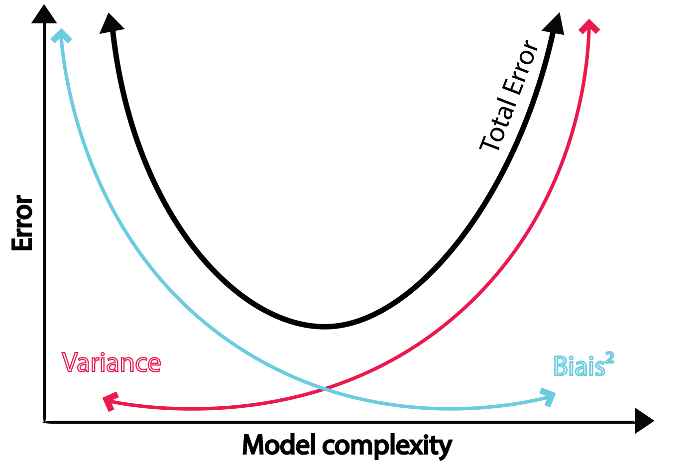
- Geman, S.; Bienenstock, E.; Doursat, R. Neural networks and the bias/variance dilemma. Neural Comput. 1992, 4, 1–58. [Google Scholar] [CrossRef]
- Breiman, L. Bias, Variance, and Arcing Classifiers; Technical Report, Tech. Rep. 460; Statistics Department, University of California: Berkeley, CA, USA, 1996. [Google Scholar]
- Strobl, C.; Boulesteix, A.L.; Zeileis, A.; Hothorn, T. Bias in random forest variable importance measures: Illustrations, sources and a solution. BMC Bioinform. 2007, 8, 25. [Google Scholar] [CrossRef] [PubMed] [Green Version]
- Al Iqbal, R. Empirical learning aided by weak domain knowledge in the form of feature importance. In Proceedings of the 2011 International Conference on Multimedia and Signal Processing, Guilin, China, 14–15 May 2011; IEEE: New York, NY, USA, 2011; Volume 1, pp. 126–130. [Google Scholar]
- Zheng, H.; Yuan, J.; Chen, L. Short-term load forecasting using EMD-LSTM neural networks with a Xgboost algorithm for feature importance evaluation. Energies 2017, 10, 1168. [Google Scholar] [CrossRef] [Green Version]
- DKA Solar Centre. Available online: http://dkasolarcentre.com (accessed on 23 September 2019).
- Pedregosa, F.; Varoquaux, G.; Gramfort, A.; Michel, V.; Thirion, B.; Grisel, O.; Blondel, M.; Prettenhofer, P.; Weiss, R.; Dubourg, V.; et al. Scikit-learn: Machine learning in Python. J. Mach. Learn. Res. 2011, 12, 2825–2830. [Google Scholar]


| Methods | Ref. | Class | Error Metrics | Lowest Error | Time Step | Data Set Location |
|---|---|---|---|---|---|---|
| PEEC | [41] | Physical | NMAE, WMAE | NMAE = 0.5% | 1-h | Politecnico di Milano |
| PMCV | [42] | Physical | RMSE, MAE, MBE | NMAE = 13% | 24-h/48-h | Hungaria |
| LSSVR–NARX | [43] | Statistical | MAE, MBE, MSE, RMSE, | = 92.03% | 2-h | Casablanca, Morocco |
| ARMAX | [8] | Statistical | RMSE, MAD, and MAPE | MAPE = 38.88% | 24-h | Coloane island of Macau |
| ARMA | [44] | Statistical | MAE, MRE | MAE = 1.16 MW | 15 min | IEEE14 bus system |
| SVM | [45] | AI | MRE, RMSE | RMSE = 1.57 MW | 24-h | PV station in China |
| CNN-LSTM | [31] | AI | MAE, RMSE, | = 99.93% | 15/45 min | Limberg, Belgium |
| RNN | [46] | AI | = 99.94% | 15–90 min | Flanders, Belgium | |
| ANN | [47] | AI | RMSE | RMSE = 0.07 KW | 24-h | Amman, Jordan |
| System Specification | Characteristics |
|---|---|
| Array rating | kW |
| Average of Powering | 141 house |
| Location | Alice Springs, Australia |
| PV technology | Crystalline Silicon, CdTe/CIGS |
| First operating installation | Since 2008 |
| Array area | 4 × 38.37 m |
| Type of tracker | Fixed: Ground Mount, Single Axis, Dual Axis |
| Inverter size/type | kW, SMA/Sunny Mini Central 6000A |
| Base Models | Hyperparameter Settings |
|---|---|
| DT | maximum depth = 3; minimum samples leaf = 3; maximum leaf nodes = 5;minimum impurity decrease = 0.2 |
| KNN | The algorithm is KDTree; the nearest neighbor number is 7; the leaf size is 90; the distance function is Minkowski distance |
| RF | The maximum depth is 50; the minimum samples split is 10; The number of estimators is 140 |
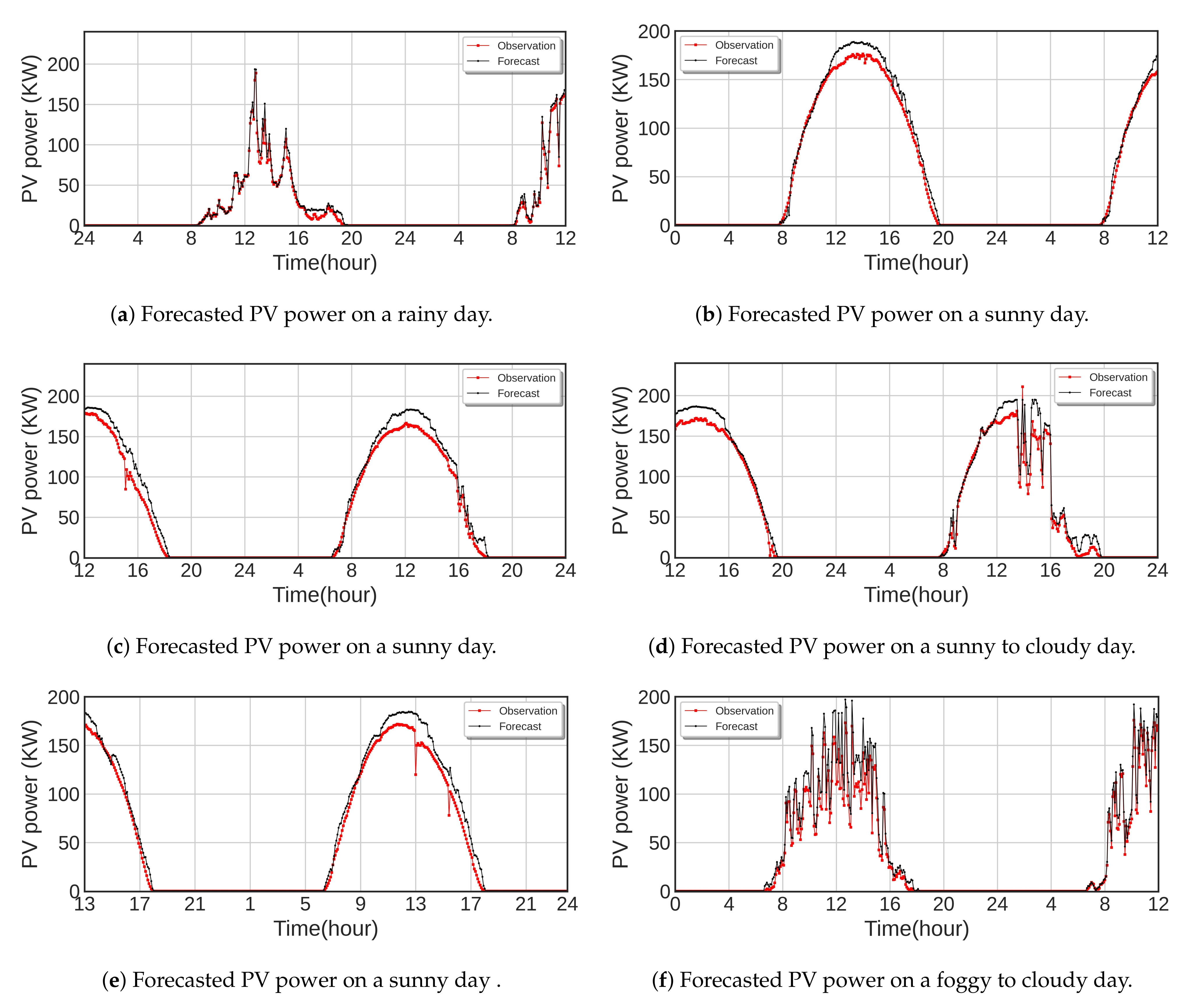
| Weather Condition | Model | RMSE (kW) ± SD | MAE (kW) ± SD |
|---|---|---|---|
| Sunny | KNN | 11.00 | 5.94 |
| RF | 12.14 | 6.70 | |
| DT | 12.41 | 6.84 | |
| Improved RF | 9.60 | 5.23 | |
| Partially cloudy | KNN | 12.74 | 8.08 |
| RF | 17.17 | 11.26 | |
| DT | 17.49 | 11.40 | |
| Improved RF | 10.79 | 6.43 | |
| Cloudy/foggy | KNN | 17.75 | 12.68 |
| RF | 19.69 | 14.00 | |
| DT | 19.96 | 14.11 | |
| Improved RF | 11.65 | 8.51 | |
| Rainy | KNN | 3.68 | 1.48 |
| RF | 8.49 | 5.00 | |
| DT | 8.84 | 5.20 | |
| Improved RF | 1.41 | 0.65 | |
| Overall | KNN | 11.29 ± 5.05 | 7.04 ± 4.03 |
| RF | 14.37 ± 4.35 | 9.24± 3.58 | |
| DT | 14.68 ± 4.33 | 9.39 ± 3.55 | |
| Improved RF | 8.36 ± 4.08 | 5.21 ± 2.88 |
Publisher’s Note: MDPI stays neutral with regard to jurisdictional claims in published maps and institutional affiliations. |
© 2021 by the authors. Licensee MDPI, Basel, Switzerland. This article is an open access article distributed under the terms and conditions of the Creative Commons Attribution (CC BY) license (https://creativecommons.org/licenses/by/4.0/).
Share and Cite
Massaoudi, M.; Chihi, I.; Sidhom, L.; Trabelsi, M.; Refaat, S.S.; Oueslati, F.S. Enhanced Random Forest Model for Robust Short-Term Photovoltaic Power Forecasting Using Weather Measurements. Energies 2021, 14, 3992. https://doi.org/10.3390/en14133992
Massaoudi M, Chihi I, Sidhom L, Trabelsi M, Refaat SS, Oueslati FS. Enhanced Random Forest Model for Robust Short-Term Photovoltaic Power Forecasting Using Weather Measurements. Energies. 2021; 14(13):3992. https://doi.org/10.3390/en14133992
Chicago/Turabian StyleMassaoudi, Mohamed, Ines Chihi, Lilia Sidhom, Mohamed Trabelsi, Shady S. Refaat, and Fakhreddine S. Oueslati. 2021. "Enhanced Random Forest Model for Robust Short-Term Photovoltaic Power Forecasting Using Weather Measurements" Energies 14, no. 13: 3992. https://doi.org/10.3390/en14133992