
Efficient Design of Energy Disaggregation Model with BERT-NILM Trained by AdaX Optimization Method for Smart Grid


Department of Electrical and Electronic Engineering, Karadeniz Technical University, Trabzon 61080, Turkey
*
Author to whom correspondence should be addressed.
Energies 2021, 14(15), 4649; https://doi.org/10.3390/en14154649
Submission received: 16 July 2021
/
Revised: 24 July 2021
/
Accepted: 28 July 2021
/
Published: 30 July 2021
(This article belongs to the Topic Innovative Techniques for Smart Grids)
Abstract
:One of the basic conditions for the successful implementation of energy demand-side management (EDM) in smart grids is the monitoring of different loads with an electrical load monitoring system. Energy and sustainability concerns present a multitude of issues that can be addressed using approaches of data mining and machine learning. However, resolving such problems due to the lack of publicly available datasets is cumbersome. In this study, we first designed an efficient energy disaggregation (ED) model and evaluated it on the basis of publicly available benchmark data from the Residential Energy Disaggregation Dataset (REDD), and then we aimed to advance ED research in smart grids using the Turkey Electrical Appliances Dataset (TEAD) containing household electricity usage data. In addition, the TEAD was evaluated using the proposed ED model tested with benchmark REDD data. The Internet of things (IoT) architecture with sensors and Node-Red software installations were established to collect data in the research. In the context of smart metering, a nonintrusive load monitoring (NILM) model was designed to classify household appliances according to TEAD data. A highly accurate supervised ED is introduced, which was designed to raise awareness to customers and generate feedback by demand without the need for smart sensors. It is also cost-effective, maintainable, and easy to install, it does not require much space, and it can be trained to monitor multiple devices. We propose an efficient BERT-NILM tuned by new adaptive gradient descent with exponential long-term memory (Adax), using a deep learning (DL) architecture based on bidirectional encoder representations from transformers (BERT). In this paper, an improved training function was designed specifically for tuning of NILM neural networks. We adapted the Adax optimization technique to the ED field and learned the sequence-to-sequence patterns. With the updated training function, BERT-NILM outperformed state-of-the-art adaptive moment estimation (Adam) optimization across various metrics on REDD datasets; lastly, we evaluated the TEAD dataset using BERT-NILM training.
1. Introduction
To meet the ever-growing energy demand, it is essential to monitor electricity power consumption and moderate its usage while increasing the production capacity. Indeed, load and energy management are essential; thus, demand-side management (DSM) with higher potentials and better results is more common. The introduction of DSM into the household sector can enable load management by both the user and the electric utility company through distinguishing the loads. For instance, controlling appliances such as cooling and heating devices with great power demand during peak hours by DSM would enable us to supply a minimum level of energy to a larger group of users. In addition, DSM [1] can help the user to understand the behavior of each device connected to the grid, facilitating both the grid and the user to better manage their energy use. The DSM intervention in large industries has also yielded good results in the form of accurate control of the load during peak hours, maximum demand control, preventing illegal actions, and implementing more accurately tariffs [2].
Nonintrusive load monitoring (NILM) of DSM is a method commonly used to predict the individual usage of home appliances on the basis of a home aggregated consumption pattern. This practically offers the ability to monitor the consumption of home appliances without the use of expensive sensors. The disaggregation of energy loads running from the power measurement over the time can be used by the electricity distribution services, as well as by the power utilities themselves, ensuring an improved user need estimation while delivering personalized services to the consumers [3]. The NILM method, introduced by Garcia et al. [4] in the mid-1980s, was the first to use transient analysis of active and reactive power for identifying the on and off states of home appliances. To date, many original research articles including several comprehensive reviews have been published on the topic [5,6]. The disaggregation process, as explained by Souza et al. [7], includes three phases: (1) the identification of events, (2) the synthesis of optimal features for classification, and (3) the energy disaggregation by real load classification.
The events related to changes in the state of home appliances were employed to synthesize features that were used for classifying the loads. Massidda et al. [8] presented a characterization based on the features sampling rate themselves, which are split to (1) less than 1 min, (2) between 1 min and 1 s, higher than 1 Hz in fundamental frequency, up to 2 kHz, and (3) between 2 and 40 kHz. The features of the categories of between 1 min and 1 s and less than 1 min can be used directly, as the statistical characterization of sub-sequences of time series [9]. Moreover, when considering the signal processing [10] in the context of previous sampling rate categorization, the high-frequency sampling rate allows characterizing more detailed transients in the consumption of home appliances [11].
In the high-frequency sampling rate, the application of signal transformation methods such as fast Fourier transform (FFT) or discrete wavelet transform (DWT) would result in the recovery of major new features fundamental for the classification [12]. The rate of high sampling frequency provides load waveform data regarding home appliances. For instance, in the trajectories of voltage–current calculation reported by Wang et al. [13], high rates of sampling allowed getting an intensive harmonic set along with the electric noise [14]. Few studies have integrated the features reproduced from the measurements of consumption with other datasets such as home appliance usage frequency [15] or weather conditions [16]. The final phase of the disaggregation operations comprises load identification from the extracted features. Many approaches have been introduced in the literature regarding this phase, which indicated challenges in the related research communities. The community first used optimization algorithms for combinatorial search [17], but the necessary computational resources limited these algorithms. The community consequently concentrated on supervised and unsupervised machine learning methods. Some methods of supervised learning with neural network (NN) architectures have been previously presented such as multilayer perceptron (MLP) [18], extreme learning machine [19], convolutional neural network (CNN) [20], and recurrent neural network (RNN) [21], as well as methods based on K-nearest neighbor (KNN) [22], support vector machine (SVM) [23], random forest classifier [24], naïve Bayes classifiers [25], and conditional random fields [26]. Unsupervised learning was principally based on the hidden Markov model (HMM) used in a related area [27]; however, clustering algorithms were also used [28]. Modern NILM methods are generally carried out by employing machine learning or optimization algorithms [29]. The strategies of pattern recognition usually fit to one-to-one matching, and yet these techniques are sensitive to noisy signal edges that can result in false detection. Optimization algorithms allow enhanced NILM performance with less sensitivity to the detection of false edges.
Machlev et al. [30] proposed evolutionary optimization approaches to identify appliances according to their given load profile. The idea of the program was that the potential appliance profiles have to be matched with the given load profile within minimum error [31]. The introduced problem concerned the Knapsack problem, which is NP-hard [32]; however, the computational performance limited its use in real-time cases because of NP-hard problem complexities. In addition, Ref. [33] introduced a DL-based NILM for edge computing on a low-cost board using the latest inference library called uTensor; this method can support any Mbed electronic board and does not require DL web API connection. In this paper, we aimed to implement BERT-based NILM (BERT-NILM) tuned by the most effective optimizer for energy disaggregation. BERT is a transformer-based machine learning technique for natural language processing and pretraining developed by Google (see Section 2); thus, two optimization models of BERT-NILM (BERT-NILM Adam and BERT-NILM AdaX) were implemented and compared for energy disaggregation systems. In training the deep learning models, Adam was used as a substitute optimization algorithm for stochastic gradient descent, whereas AdaX improved upon Adam by proposing a novel adaptive gradient descent algorithm. Unlike Adam, which ignores the past gradients, AdaX exponentially accumulates the long-term gradient information during training to adaptively tune the learning rates (see Section 2.4 and Section 2.5). The REDD and TEAD datasets were used for training and validating the effectiveness of the designed models. This study introduced ED methods that track energy efficiency, using detailed energy data to take measures to reduce consumption through nonintrusive “energy awareness”, which can be activated if smart meters are already installed. It can also provide information on domestic activities that are becoming an alternative emerging technology for use in healthcare sectors.
The manuscript is organized as follows: Section 1 reviews the architecture of BERT-NILM, Section 2 deals with the NILM benchmark datasets; Section 3 presents several model evaluations and metrics; Section 4 provides a discussion of the results and conclusions of the important characteristics of the study.
1.1. Architecture of BERT-NILM
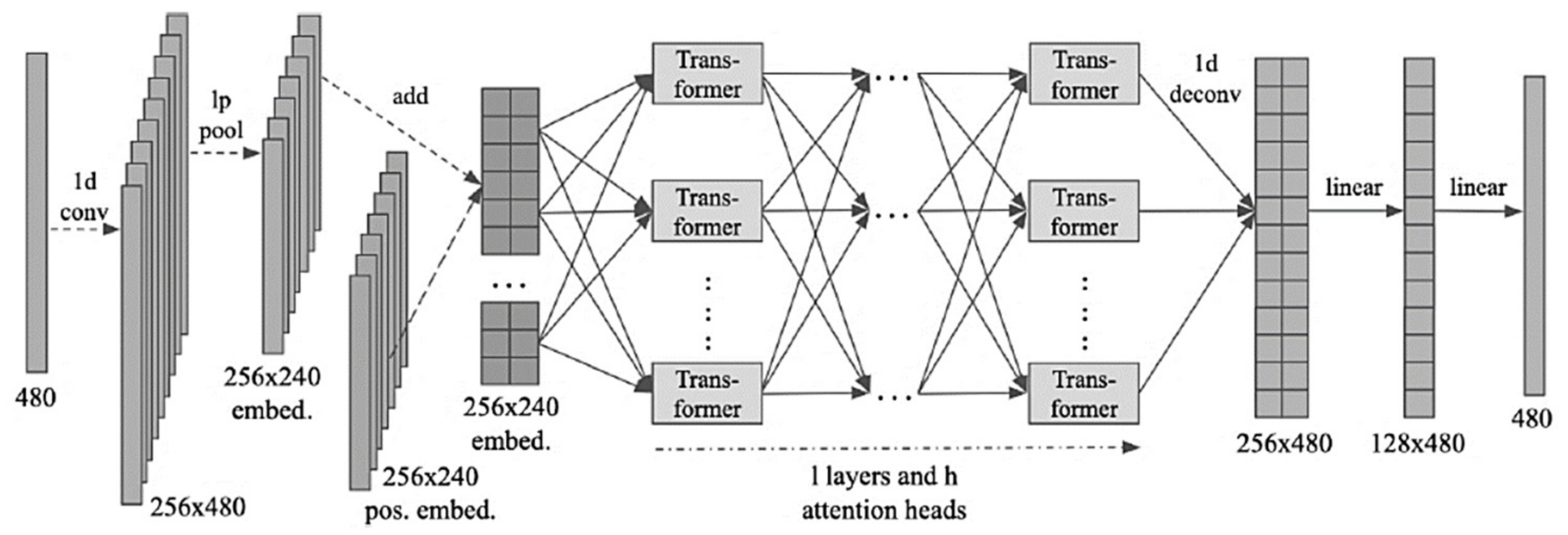
As shown in Figure 1, the proposed BERT [34] architecture consists of an embedding module, layers of transformers, and a multilayer perceptron output layer (MLP). The network was supplied with fixed-length sequential data to categorize individual home appliances with the same shape output. In addition, threshold values were calculated by comparison of electrical appliances. The features were initially extracted from the architecture by adopting a convolutional layer to increase the hidden size of the one-dimensional input array prior to feeding the input data to the blocks of transformers. We then pooled the convolutional output with increased hidden size using a learned L2 norm pooling operation. The operation enforces squared-average pooling over the input sequence to better maintain the features while reducing the length by half. We then added the pooled input to a learnable positional embedding matrix. The matrix takes sequence positional encoding into account, where Embeddi(X) = LPPooling (conv(X)) + epose.
Furthermore, we operated the analysis by supplying the bidirectional transformer with the final embedding matrix. The transformer consisted of l layers of transformers and h attention heads within each layer. The single-head self-attention (scaled dot-product attention) could be formulated with Q(Query), K(Key), and V(Value) matrices (obtained by linear transformation of the input matrix). Q and K (initially multiplied and divided by the squared root of the hidden size) were processed by a softmax operation to build soft attention prior to being multiplied by V, yielding a weighted value matrix. Comparably, multi-head attention would divide the hidden space into multiple subspaces with parameter matrices performing identical computation, resulting in several Q, K, and V matrices. Each of the factors with individual attention could retrieve information from different subspaces. Outcomes were integrated and transformed to form the attentive output, where attention (Q) = softmax (QKT/√dk)V.
Multi-head (Q, K, V) = concat(head1, head2, …, headh) WO, where headi = attention(QWQi, KWKi, VWVi). Additionally, we supplied a position-wise feed-forward network (PFFN) with the previous matrix after the multi-head attention in each transformer layer. It is of note that the layer processes input elements with linear transformations and Gaussian error linear unit (GELU) activation. UC Berkeley’s Dan Hendrycks and Kevin Gimpel introduced the GELU activation function in 2018 from the Toyota Technological Institute at Chicago [35]. An activation function is the “switch” that triggers neuron output, and its importance has grown as networks have deepened. To preserve input features, following the attention and feed-forward modules, residual connections were applied. Subsequently, we performed layer normalization (LayerNorm) to stabilize the hidden state dynamics between various layers. The operation can be formulated as follows: LayerNorm(x + Dropout (Module (x))), PFFN (X) = GELU(0,XW1 + b1)W2 + b2.
After passing the values through transformer layers, the output MLP can be found, including a deconvolutional layer and two linear layers. The deconvolutional (inverse to convolution) layer first develops the output to its previous length with transposed convolution. Subsequently, a two-layer MLP with Tanh activation in between would reinstate the hidden size of the input to the desired output size. Output values (preferably in the interval [0, 1]) were multiplied with the maximal device power and then secured to construct reasonable energy prediction, while attaining the status of appliance by matching corresponding on thresholds, where Ou(X) = Tanh(Deconv(X)W1 + b1)W2 + b2.
1.2. Energy Disaggregation NILM Background
Given a smart meter (SM), with an aggregate power consumption series P = {p1, p2, p3, …, pt} for time T = {1, 2, 3, …, t}, the NILM problem can formulated as follows [36]:
where σ(t) is unaccounted noise, used to infer the consumption power of home appliance i ∈ {1, 2, 3, …, M} of the M active appliances.
An NILM system includes four stages, as illustrated in Figure 2: signal power acquisition with preprocessing, event detection with feature extraction, inference with learning, and appliance classification. The first stage of energy disaggregation is signal power acquisition, and its task is acquiring aggregated load measurements at varying sampling rates. The event detection and feature extraction stage involves setting the transient or steady state in the preprocessed power measurements. Features related to the extracted events are unique patterns of consumption related to each appliance activity. In the stage of learning and inference, the essential supervised/unsupervised techniques are applied to identify the appliances. At the final stage, the classification of appliances consists of splitting the total aggregate recordings into the power consumption and individual appliance states related to that appliance state [37].
2. NILM Benchmark Dataset
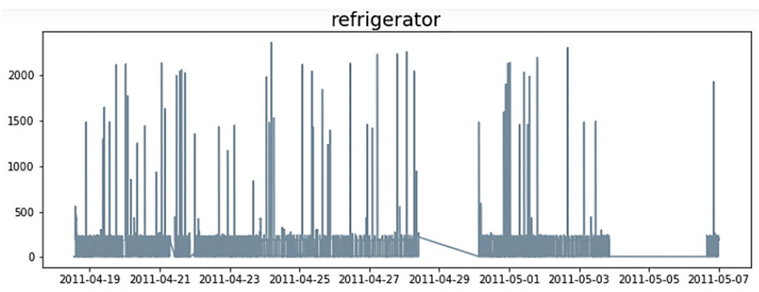
In this study, we used the Residential Energy Disaggregation Dataset (REDD) [38] for energy disaggregation. This NILM dataset is publicly available containing measured power consumption data from real-world environments such as houses or buildings. The dataset includes smart metering data and may have an individual device ground truth for power consumption data based on the dataset goals. To evaluate the performance of an NILM algorithm, with respect to an appliance for which the disaggregation is performed, it is necessary to have the ground truth. Figure 3 shows the plot of refrigerator data for the first 2 days of REDD house 1.
Figure 4 illustrates the data separation for training and testing. The refrigerator was chosen as a known device for training the BERT network of NILM. In house 1, data were separated into training and testing. The training data involved 17 usage days of power data, whereas testing data involved 6 days. After training the disaggregation network, we used the data from house 2 to validate the performance efficiency of the NILM network as an unknown device.
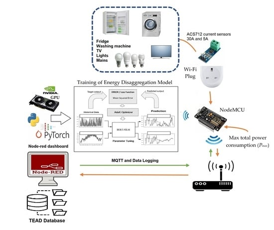
2.1. IOT Structure of Data Collecions
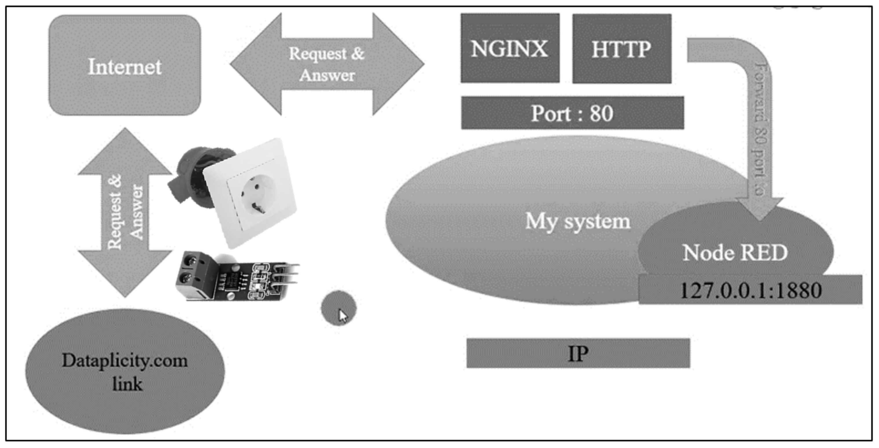
In this study, a data collection architecture was designed using the IoT. Node-Red was used in the software part of the system. Node-Red is built on top of NodeJS and takes full advantage of its event-driven, non-blocking model, running on web browsers. We set up a port forwarding structure as illustrated in Figure 5 on a Linux Ubuntu PC using the NGINX server to access the system from any web browser over the internet remotely.
The IoT structure consisted of sensors and actuators for monitoring and control; accordingly, we measured the power consumed by current sensors attached to electrical household appliances in this research and created a dataset for classifying devices with artificial intelligence.
The materials used were as follows:
- -
- NodeMCU ESP8266 (WiFi),
- -
- Modem (WiFi),
- -
- Ubuntu PC (server) or Raspberry Pi,
- -
- ACS-712 (30A and 5A current sensors).
2.2. Loss Function
Another parameter of evaluating such models is the loss or error function. When the prediction output diverges too much from the real target results, the loss function can be used to optimize target results. The loss function learns to minimize the error in predictions when an optimization algorithm is applied. In this study, we used the mean square error (MSE) [39], which is the sum of squared distances between the predicted and target results to reduce the errors.
2.3. Optimization Function
Many studies have used the state-of-the-art adaptive moment estimation (Adam) algorithm as the optimization function. Adam is an optimization method used to improve the gradient descent (GD) with iterative neural weights, which is updated on the basis of the training data. Adam is the preferred algorithm for DL since it can rapidly produce fine results and boost the computation efficiency. Although Adam demonstrates fast convergence when using many machine learning (ML) approaches, this study aimed to improve Adam using a novel adaptive gradient descent named AdaX. Adam ignores the past gradients, but AdaX exponentially accumulates the long-term gradient data during training while adjusting the learning rate adaptively. We demonstrate the convergence of AdaX in BERT disaggregator settings.
2.4. Adam Optimization Algorithm
The Adam [40] optimizer computes the learning rate (LR) as a function of data by storing the exponential mean reduction in previous gradients sums (vt) such as AdaDelta and RMSprop [41], which keeps the exponential mean reduction in mt gradients similarly to an acceleration technique.
where mt and vt are the first moment estimates as means and second moment estimates as the decentralized variance of gradients, respectively. Since the primary state of the vectors mt and vt is zero, the developers found that the results are tilted toward zero. This was more evident in early steps with a small reduction rate (i.e., β1 and β2 were close to 1). To solve the problem, they used corrected estimates of the first and second estimates [41].
These two formulas, similarly to AdaDelta and RMSprop, were used to compute changes in the parameters, thus obtaining the following formula of changes:
The proposed default values of β1, β2, and ϵ are 0.9, 0.999, and 10−8, respectively. The developers experimentally showed that the Adam method outperforms other adaptive learning methods.
2.5. AdaX Optimizer Algorithm
This study introduces a novel BERT energy disaggregator by adjusting the adaptive learning rate. According to the discussions by Li et al. [42], small gradients can produce an unstable second moment and, thus, past memory should be highlighted similarly to the max operation in AMSGrad [43]. Furthermore, the highlighted operation should not be duty-dependent to prevent the exponential reduction in gradients. Unlike the Adam algorithm, in the proposed NILM-AdaX, adjustment was done by assigning exponentially greater weights to the past gradients and progressively reducing the current gradients in an adaptive manner, as presented in Algorithm 1 by Li et al. The most significant differences between AdaX and Adam can be seen in the lines six and seven, where, instead of using an exponential moving average, (β2, 1 − β2) was changed to (1 + β2, β2) in the design.
| Algorithm 1. AdaX Algorithm |
| 1: Input: x ∈ F, {αt} (β1, β2) = (0.9, 10−4) |
| 2: Initialize m0 = 0, v0 = 0 |
| 3: for t = 1 to T do |
| 4: gt = ∇ft(xt) |
| 5: mt = β1mt − 1 + (1 − β1)gt |
| 6: vt = (1 + β2)vt−1 + β2 |
| 7: = vt/[(1 + β2) t − 1] and Vt = diag() |
| 8: xt + 1 = ΠF, √ Vt (xt − αtmt/√ ) |
| 9: end for |
Line 6 shows that the past gradients are multiplied by a constant greater than one, which means that past data have been accumulated rather than overlooked. Every is multiplied by a small number and added to the past memory. The idea behind the algorithm is to progressively reduce the second moment adaptively toward the newest gradients as they scatter and become noisy, while the parameters stay near the optimal values, as presented in the synthetic model by Li et al. In the current study, the proposed design ensures the noninterference of small gradients on the update steps when vt is kept large. Accordingly, with the bias correction term, the proposed progressively becomes big and stable. In line 7, to achieve an unbiased prediction of the second moment, vt was divided by the term of bias correction. As shown in the derivation of Kingma and Ba [44], the gradient gt at time step t can be drawn from a gt∼p (gt) stationary distribution, thus yielding
Hence, to maintain the accuracy of the second moment, vt was divided by (1 + β2)t − 1 in line 7. Nevertheless, in Kingma and Ba, the first term of moment correction (1 − ) was not involved for the above reason. The stochastic gradient descent with momentum (SGDM) and the first moment of Adam can be calculated as
2.6. Proposed Disaggregator on Supervised Learning Structure
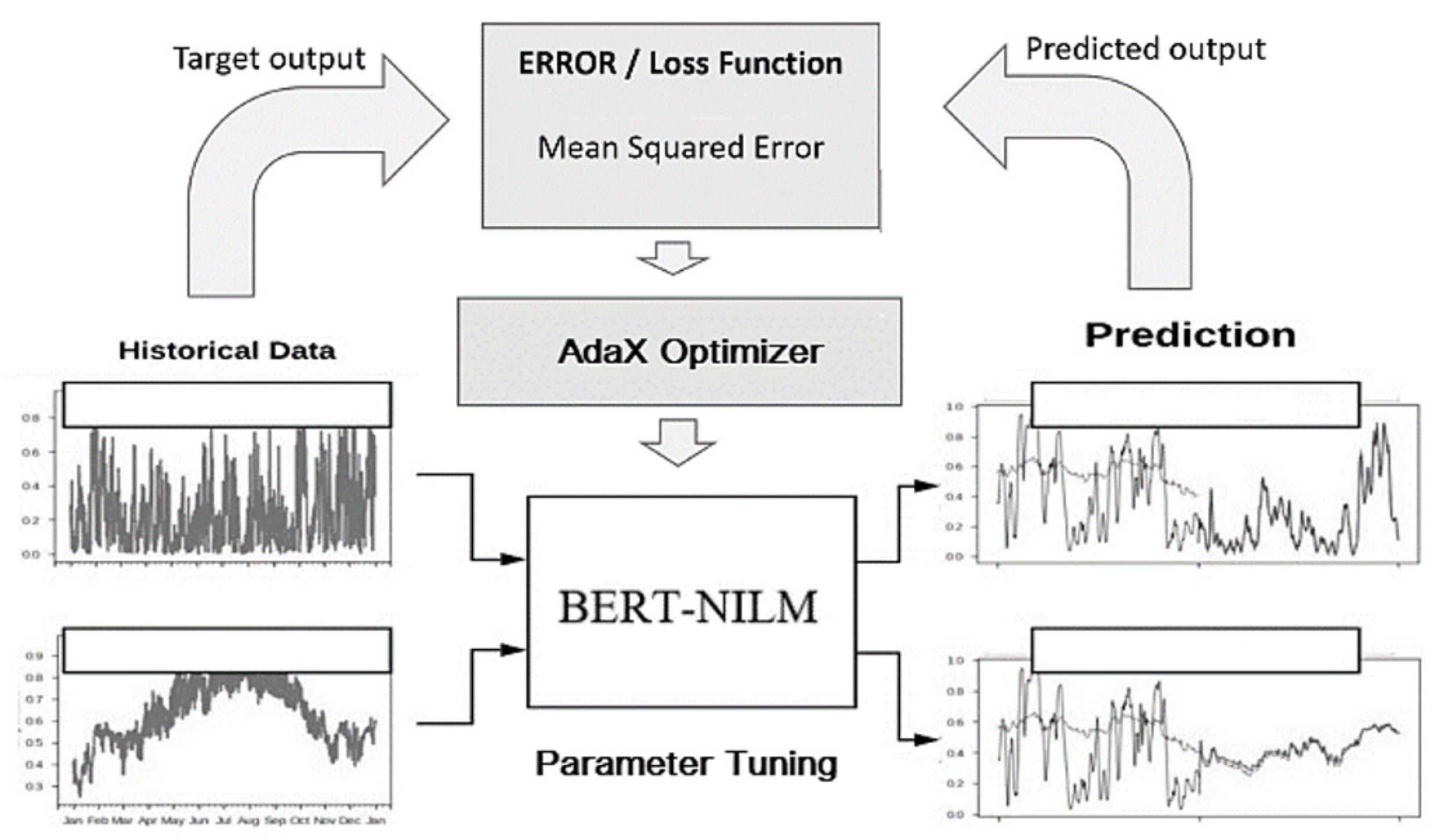
The proposed BERT-NILM model features a supervised learning method to calculate the minimum prediction error using an iterative process for the given training data. The error is generally expressed as the difference between model-predicted output and actual/target output, which is given as a part of training data. The proposed disaggregator consists of a loss function, an optimization method, and the BERT-NILM model. The loss function proposed by Çimen et al. is presented in equation, the optimization algorithm is explained in Section 2.5, and the designed BERT architecture is illustrated in Figure 6.
3. Model Evaluations and Metrics
Metrics [44] of model evaluation allow quantifying model performance. In this study, we used root-mean-square error (MSE) and accuracy. The RMSE defined as follows [45]:
Different metrics can be used to evaluate NILM methods, making it difficult to compare evaluations on the basis of different methods and algorithms for load monitoring. At first, when the algorithms are applied with two modes (on/off), the evaluation criteria are based on the percentage of correct load classifications for a notable change in total used power. There are various criteria [46] used for this purpose, and the following variables need to be defined before introducing them:
TP (total number of real positives): when both the device and ground truth are on.
FP (total number of fake positives): when the device is on and ground truth is off.
TN (total number of real negatives): when both the device and ground truth are off.
FN (total number of fake negatives): when the device is off and ground truth is on.
P: total number of positives on ground truth.
N: total number of negatives on ground truth.
Accuracy: the ratio of real results in all cases.
Regarding precision and ED, this metric indicates what percentage of the total energy assigned to a device is actually used by that device.
The F1 score is the harmonized mean accuracy and recall.
Recall, regarding the ED, is part of the correctly classified and measured energy.
3.1. Experiments
To determine the impact of adaptive learning rate (LR) on neural network (NN) performance, we first evaluated the performance of ADAM as a recent optimization algorithm in comparison with AdaX on the proposed BERT-NILM model using the REDD. We evaluated the AdaX technique as a function of performance metrics for the ADAM-trained BERT-NILM [47], where the results showed that AdaX was superior to Adam for the BERT-NILM disaggregation problem. AdaX performance was also evaluated for BERT-NILM using the TEAD [48].
In the context of efficient backpropagation, LR is a hyperparameter that controls how much the NN model is changed in response to the predicted error each time the NN model weights are updated. Selecting the LR rate is a challenging issue [49], whereby choosing too small LR rates may result in long training procedures that could become stuck, and choosing too large LR rates may result in an unstable training procedure or learning a suboptimal set of weights too fast. With respect to BERT, while the model architectures are evolving continually, the training algorithms have remained rather constant, i.e., stochastic gradient descent (SGD) methods. SGD is a method for optimizing a cost function in an iteration loop with convenient smoothness properties [50]. The momentum technique was later naturally integrated into SGD algorithms, and this method remains the standard training regime for BERT [51]. Despite the improvements of implementation, SGD algorithms have disadvantages that limit further improvements in training. The first disadvantage is that hyperparameters such as LR and convergence criteria need to be tuned manually. The second disadvantage is that, unlike batch learning, SGD algorithms have little room for serious optimization because one sample with a noisy nature per iteration renders the output unreliable for further optimization. The third disadvantage is that SGD algorithms are inherently sequential and are exceptionally challenging to parallelize using GPUs or to be distributed with a computer cluster [52].
For validating the proposed model, we split the REDD data into a validation set for training and testing the obtained model. In Table 1, the metrics presented are the mean accuracy (MA), mean precision (MP), mean recall (MR), mean F1 score (MF1), mean relative error (MRE), and mean absolute error (MAE) of the fridge, washer/dryer, microwave, and dishwasher. Table 3 presents the model performances using the REDD, where the MP and MR metrics are not included in the comparison.
The data chosen for training the BERT-NILM from house 1 involved 17 usage days of power data, whereas 6 days of data were used for testing. Table 1 indicates that the BERT-NILM network with the AdaX optimizer could achieve a better average performance for all devices using the test data from house 2, presenting an MA of 0.95, MP of 0.54, MR of 0.74, MF1 of 0.58, MRE of 0.24, and MAE of 26.49. The BERT-NILM network with Adam obtained an MA of 0.94, MF1 of 0.57, MRE of 0.23, and MAE of 26.35.
Table 2, highlighting the fridge metrics, indicates that the BERT-NILM tuned with AdaX could achieve a better performance than that tuned with Adam using the test data from house 2, presenting an MA of 0.89, MP of 0.71, MR of 0.98, MF1 of 0.82, MRE of 0.81, and MAE of 29.75. The BERT-NILM tuned with Adam obtained an MA of 0.84, MF1 of 0.75, MRE of 0.80, and MAE of 32.35.
Table 3, highlighting the washer/dryer metrics, shows that the BERT-NILM trained by AdaX performed better than that trained by Adam using the test data from house 2, presenting an MA of 0.971, MP of 0.68, MR of 0.36, MF1 of 0.47, MRE of 0.04, and MAE of 25.16. The BERT-NILM trained by Adam obtained an MA of 0.84, MF1 of 0.52, MRE of 0.039, and MAE of 20.49.
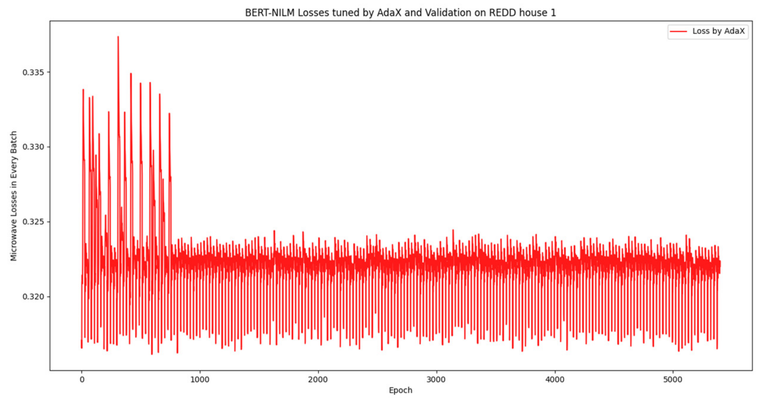
Table 4, highlighting the microwave metrics, demonstrates that the BERT-NILM trained by Adam performed better than that trained by AdaX using the test data from house 2, presenting an MA of 0.97, MP of 0.32, MR of 0.71, MF1 of 0.45, MRE of 0.07, and MAE of 20.56. The BERT-NILM trained by Adam obtained an MA of 0.88, MF1 of 0.47, MRE of 0.05, and MAE of 17.58.
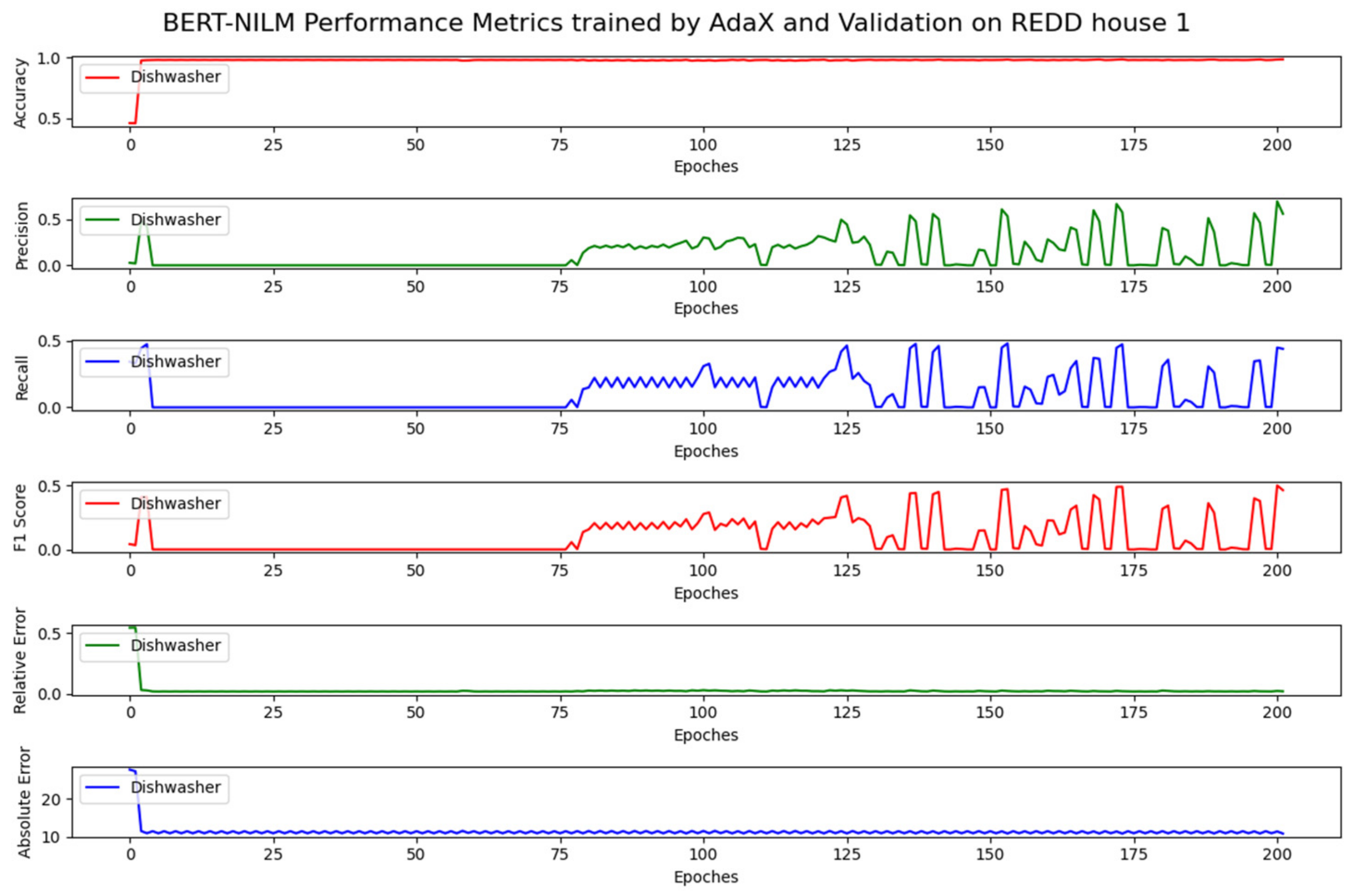
Table 5, highlighting the dishwasher metrics, indicates that the BERT-NILM trained by AdaX performed equally to that trained by Adam using the test data from house 2, presenting an MA of 0.96, MP of 0.68, MR of 0.36, MF1 of 0.47, MRE of 0.04, and MAE of 25.16. The BERT-NILM trained by Adam obtained an MA of 0.96, MF1 of 0.52, MRE of 0.03, and MAE of 20.49. The proposed model tuned the hyperparameters to run on an Nvidia 2070 RTX Super GPU.
Graphics shows the training progress of BERT-NILM based on REDD. Figure 7: Shows Fridge losses of training process and validation sets on house 1. Figure 8: About Fridge metrics according to AdaX and validation on house 1. Figure 9: Graphs washer/dryer losses of BERT training and validation sets on house 1. Figure 10: Shows washer/dryer metrics of AdaX and validation on house 1. Figure 11: About microwave losses of BERT training and validation sets on house 1. Figure 12: Is microwave metrics of AdaX and validation on house 1. Figure 13: Graphs dishwasher losses of BERT training and validation sets on house 1. Figure 14: About dishwasher metrics of AdaX and validation on house 1.
3.2. TEAD Evaluations on BERT-NILM
For evaluating the proposed dataset, we split the TEAD data into validation and training sets. Table 6 presents the metrics for the TV, washing machine, lights, and fridge.
Table 6 indicates that the TEAD-based BERT-NILM trained by AdaX performed better than that trained by Adam in terms of MA and MP, presenting an MA of 0.86, MP of 0.86, MR of 0.93, MF1 of 0.89, MRE of 0.35, and MAE of 23.42.
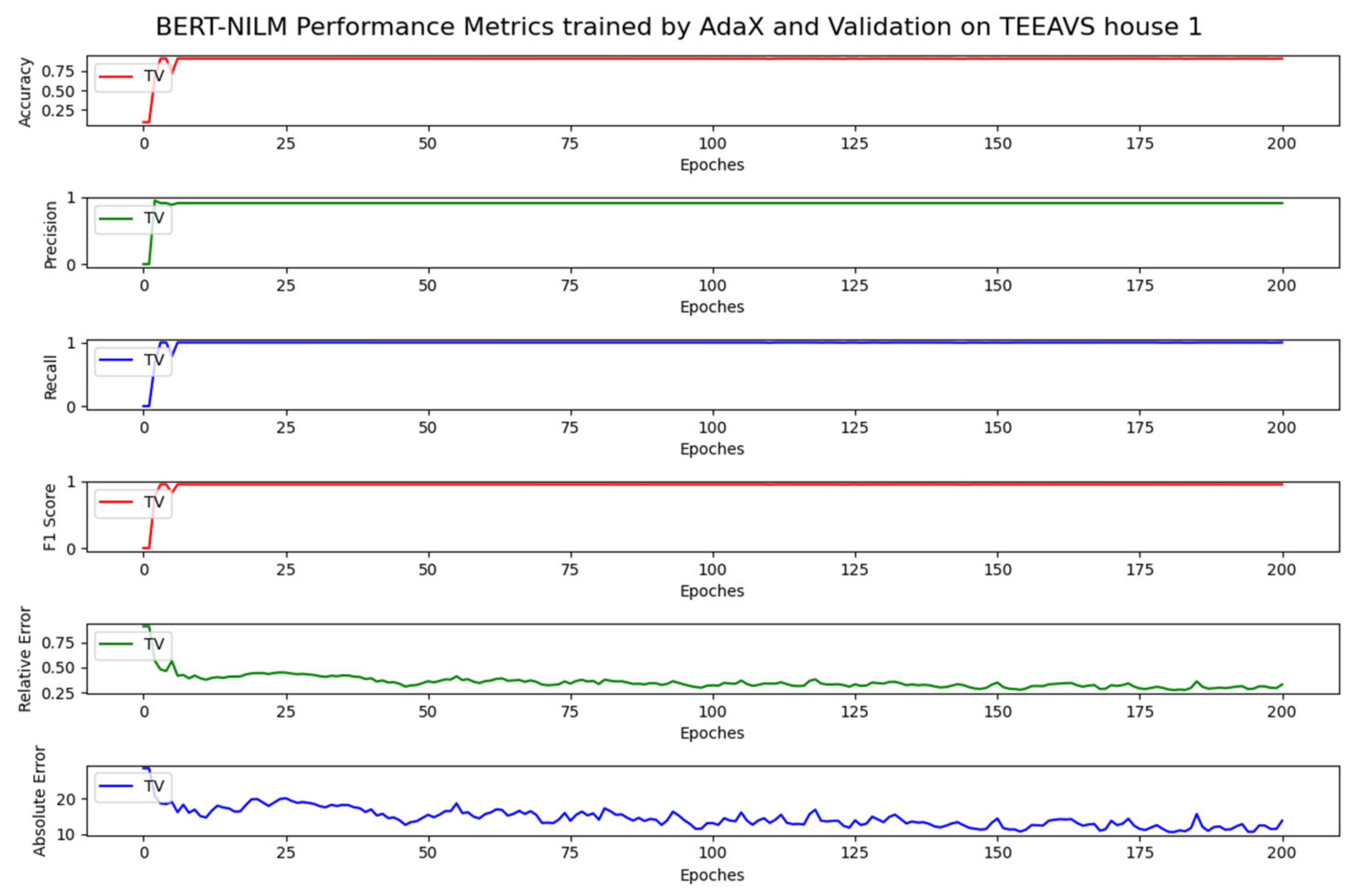
Table 7, highlighting the TV metrics, indicates that the TEAD-based BERT-NILM tuned by AdaX performed almost equally to that trained by Adam, presenting an MA of 0.92, MP of 0.92, MR of 0.99, MF1 of 0.96, MRE of 0.18, and MAE of 5.47.
Table 8, highlighting the fridge metrics, indicates that the TEAD-based BERT-NILM tuned with AdaX performed almost equally to that tuned with Adam, but better in terms of MR, presenting an MA of 0.92, MP of 0.92, MR of 1, MF1 of 0.96, MRE of 0.43, and MAE of 54.22.
Table 9, highlighting the metrics for lights, indicates that the TEAD-based BERT-NILM tuned with AdaX performed almost equally to that tuned with Adam, presenting an MA of 0.99, MP of 0.99, MR of 1, MF1 of 0.99, MRE of 0.29, and MAE of 20.69. The increased activities of lights during the day with a resistive load profile could provide good training results.
Table 10, highlighting the washing machine metrics, indicates that the TEAD-based BERT-NILM tuned with Adax performed better than that tuned with Adam in terms of MA and MP, presenting an MA of 0.60, MP of 0.61, MR of 0.72, MF1 of 0.66, MRE of 0.51, and MAE of 13.32. The washing machine in TEAD was less active during the day, resulting in a lack of feature data representing the target device; thus, REDD was better than TEAD in terms of the model training experiments.
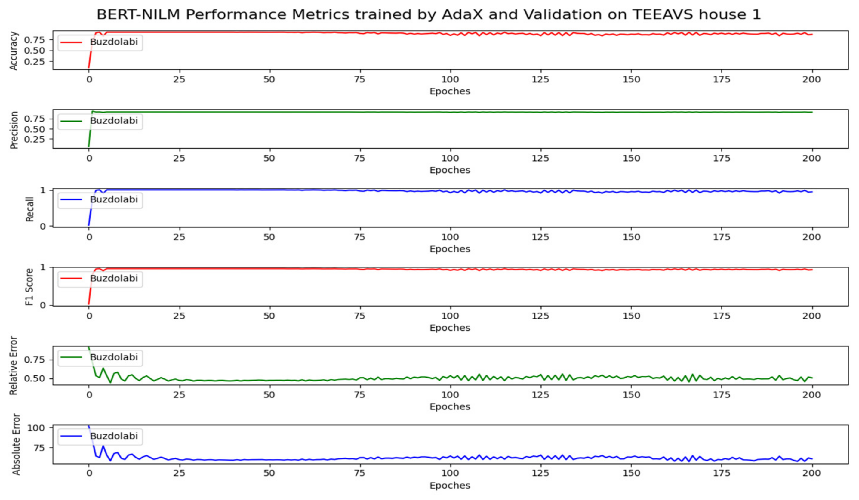
Graphics shows the training progress of BERT-NILM based on TEAD. Figure 15: Shows TV losses of BERT training and validation sets on house 1. Figure 16: About TV metrics of AdaX and validation on house 1. Figure 17: Graphs fridge losses of BERT training and validation sets on house 1. Figure 18: About fridge metrics of AdaX and validation on house 1. Figure 19: Shows losses for lights of BERT training and validation sets on house 1. Figure 20: Are metrics for lights according to AdaX and validation on house 1. Figure 21: Graphs washing machine losses of BERT training and validation sets on house 1. Figure 22: About washing machine metrics of AdaX and validation on house 1.
4. Conclusions
In summary, this paper reviewed the literature on the deep neural net-based NILM. The review comprised several studies that used deep learning and efficient optimization methods for the ED of home appliances through low-frequency data, i.e., sampling rates data lower than the alternative current (AC) frequency. Our motivation for this study was that many of papers could benefit from a well-trained NILM, integrated with IoT developments, as low-frequency data will be available at scale in the near future and there has been tremendous deep learning success in other application domains. Energy and sustainability issues can be addressed using data mining and machine learning approaches. However, such problems have been resolved slowly due to the lack of publicly available datasets. In this study, the Turkey Electrical Appliances Dataset (TEAD) was presented, which includes electricity usage information collected from houses aimed at advancing energy disaggregation (ED) research in smart grids. In the context of smart metering, a NILM model was proposed to classify household appliances as a function of TEAD information. The NILM system enables using production assets more efficiently via reducing the energy demand of users by providing detailed feedback and awareness during demand-side heavy loads. Thus, end users will be able to obtain detailed billing with highly accurate supervised ED by demand, without the need for expensive smart socket sensors. Benefits of the proposed ED are its energy efficiency and itemized energy data used to reduce energy consumption through a system of energy awareness with NILM, which can be deployed on already installed smart meters. Disadvantages are that continuously variable appliance cannot be detected, electrically identical (similar in every detail) appliances cannot be distinguished, there is a greater potential for undetected error, and it is difficult to recognize unusual appliances.
In this paper, we presented an efficient energy disaggregator with a BERT model tuned with the AdaX optimization algorithm to improve the performance of conventional NILM methods. We first extend Adam’s fast convergence by considering AdaX. We then propose AdaX (an optimizer with “long-term memory”) applied to BERT-NILM, analyze its convergence, and evaluate its performance in learning signals of the energy disaggregation task. Our analysis and experimental results demonstrated that the designed disaggregator model tuned with AdaX performed better than the recent Adam optimizer in the energy disaggregation task based on BERT. It is of note that more research is warranted for the evaluation of total performance of NILM. Additionally, the current study represents but the first step in designing efficient energy disaggregation methods beyond the simple NILM approaches. However, other novel designs should also be examined for a concrete statement. In the context of modern deep leaning and efficient backpropagation, we believe that new optimization algorithms with a long-term cache of gradients for performing adaptive learning may outperform AdaX on NILM tasks; however, their its convergence and performance need to be thoroughly investigated.
Author Contributions
V.F. collected the data for this study; İ.H.Ç. developed the original hypotheses and designed the experiments. All authors read and agreed to the published version of the manuscript.
Funding
This research received no external funding.
Institutional Review Board Statement
Not applicable.
Informed Consent Statement
Not applicable.
Data Availability Statement
The data presented in this study are available at https://github.com/vahit19/smart_grid.
Acknowledgments
The article was extracted from the PhD thesis prepared by Vahit Feryad under the supervision of İsmail Hakkı Çavdar.
Conflicts of Interest
The authors declare no conflict of interest.
Nomenclature
| MA | Mean accuracy |
| MP | Mean precision |
| MR | Mean recall |
| MF1 | Mean F1 score |
| MRE | Mean relative error |
| MAE | Mean absolute error |
| σ(t) | Unaccounted noise |
| Consumption power | |
| MSE | Mean square error |
| LR | Learning rate |
| mt | First moment |
| vt | Second moment |
| β1, β2 | Initial decay rates in the first and second moments of the gradient |
| gt | Gradient of losses |
| “Cache” of past weight values which decay over time | |
| η | Learning step size |
References
- Gelazanskas, L.; Gamage, K.A. Demand side management in smart grid: A review and proposals for future direction. Sustain. Cities Soc. 2014, 11, 22–30. [Google Scholar] [CrossRef]
- Behrangrad, M. A review of demand side management business models in the electricity market. Renew. Sustain. Energy Rev. 2015, 47, 270–283. [Google Scholar] [CrossRef]
- Athanasiadis, C.; Doukas, D.; Papadopoulos, T.; Chrysopoulos, A. A Scalable Real-Time Non-Intrusive Load Monitoring System for the Estimation of Household Appliance Power Consumption. Energies 2021, 14, 767. [Google Scholar] [CrossRef]
- Garcia, F.D.; Souza, W.A.; Diniz, I.S.; Marafão, F.P. NILM-based approach for energy efficiency assessment of household appliances. Energy Inform. 2020, 3, 1–21. [Google Scholar] [CrossRef]
- Gopinath, R.; Kumar, M.; Joshua CP, C.; Srinivas, K. Energy management using non-intrusive load monitoring techniques-State-of-the-art and future research directions. Sustain. Cities Soc. 2020, 62, 102411. [Google Scholar] [CrossRef]
- Moradzadeh, A.; Sadeghian, O.; Pourhossein, K.; Mohammadi-Ivatloo, B.; Anvari-Moghaddam, A. Improving residential load disaggregation for sustainable development of energy via principal component analysis. Sustainability 2020, 12, 3158. [Google Scholar] [CrossRef] [Green Version]
- de Souza, W.A.; Garcia, F.D.; Marafão, F.P.; Da Silva LC, P.; Simões, M.G. Load disaggregation using microscopic power features and pattern recognition. Energies 2019, 12, 2641. [Google Scholar] [CrossRef] [Green Version]
- Massidda, L.; Marrocu, M.; Manca, S. Non-Intrusive Load Disaggregation by Convolutional Neural Network and Multilabel Classification. Appl. Sci. 2020, 10, 1454. [Google Scholar] [CrossRef] [Green Version]
- Kalluri, B.; Kamilaris, A.; Kondepudi, S.; Kua, H.W.; Tham, K.W. Applicability of using time series subsequences to study office plug load appliances. Energy Build. 2016, 127, 399–410. [Google Scholar] [CrossRef]
- Zhao, B.; He, K.; Stankovic, L.; Stankovic, V. Improving event-based non-intrusive load monitoring using graph signal processing. IEEE Access 2018, 6, 53944–53959. [Google Scholar] [CrossRef]
- Meziane, M.N.; Picon, T.; Ravier, P.; Lamarque, G.; Le, J. A new measurement system for high frequency NILM with controlled aggregation scenarios. Available online: http://nilmworkshop.org/2016/proceedings/Poster_ID23.pdf (accessed on 30 July 2021).
- Sadeghianpourhamami, N.; Ruyssinck, J.; Deschrijver, D.; Dhaene, T.; Develder, C. Comprehensive feature selection for appliance classification in NILM. Energy Build. 2017, 151, 98–106. [Google Scholar] [CrossRef] [Green Version]
- Wang, A.L.; Chen, B.X.; Wang, C.G.; Hua, D. Non-intrusive load monitoring algorithm based on features of V–I trajectory. Electr. Power Syst. Res. 2018, 157, 134–144. [Google Scholar] [CrossRef]
- Ruano, A.; Hernandez, A.; Ureña, J.; Ruano, M.; Garcia, J. NILM techniques for intelligent home energy management and ambient assisted living: A review. Energies 2019, 12, 2203. [Google Scholar] [CrossRef] [Green Version]
- Çimen, H.; Çetinkaya, N.; Vasquez, J.C.; Guerrero, J.M. A Microgrid Energy Management System based on Non-Intrusive Load Monitoring via Multitask Learning. IEEE Trans. Smart Grid 2020, 12, 977–987. [Google Scholar] [CrossRef]
- Elahe, M.F.; Jin, M.; Zeng, P. Review of load data analytics using deep learning in smart grids: Open load datasets, methodologies, and application challenges. Int. J. Energy Res. 2021, 45, 14274–14305. [Google Scholar] [CrossRef]
- Hernández, Á.; Ruano, A.; Ureña, J.; Ruano, M.G.; Garcia, J.J. Applications of NILM techniques to energy management and assisted living. IFAC-Pap. 2019, 52, 164–171. [Google Scholar] [CrossRef]
- de Paiva Penha, D.; Castro, A.R.G. Home appliance identification for NILM systems based on deep neural networks. Int. J. Artif. Intell. Appl. 2018, 9, 69–80. [Google Scholar] [CrossRef]
- Salerno, V.M.; Rabbeni, G. An extreme learning machine approach to effective energy disaggregation. Electronics 2018, 7, 235. [Google Scholar] [CrossRef] [Green Version]
- Yu, J.; Zhang, C.; Wang, S. Multichannel one-dimensional convolutional neural network-based feature learning for fault diagnosis of industrial processes. Neural Comput. Appl. 2021, 33, 3085–3104. [Google Scholar] [CrossRef]
- Bai, Y.; Xie, J.; Liu, C.; Tao, Y.; Zeng, B.; Li, C. Regression modeling for enterprise electricity consumption: A comparison of recurrent neural network and its variants. Int. J. Electr. Power Energy Syst. 2021, 126, 106612. [Google Scholar] [CrossRef]
- Himeur, Y.; Alsalemi, A.; Bensaali, F.; Amira, A. Smart power consumption abnormality detection in buildings using micromoments and improved K-nearest neighbors. Int. J. Intell. Syst. 2021, 36, 2865–2894. [Google Scholar] [CrossRef]
- Singh, M.; Kumar, S.; Semwal, S.; Prasad, R.S. Residential load signature analysis for their segregation using wavelet—SVM. In Power Electronics and Renewable Energy Systems; Springer: New Delhi, India, 2015; pp. 863–871. [Google Scholar] [CrossRef]
- Chowdhury, D.; Hasan, M.M. Non-Intrusive Load Monitoring Using Ensemble Empirical Mode Decomposition and Random Forest Classifier. In Proceedings of the International Conference on Digital Image and Signal Processing (DISP), Oxford, UK, 29–30 April 2019; pp. 29–30. [Google Scholar]
- Yang, C.C.; Soh, C.S.; Yap, V.V. A non-intrusive appliance load monitoring for efficient energy consumption based on Naive Bayes classifier. Sustain. Comput. Inform. Syst. 2017, 14, 34–42. [Google Scholar] [CrossRef]
- Saha, D.; Bhattacharjee, A.; Chowdhury, D.; Hossain, E.; Islam, M.M. Comprehensive NILM Framework: Device Type Classification and Device Activity Status Monitoring Using Capsule Network. IEEE Access 2020, 8, 179995–180009. [Google Scholar] [CrossRef]
- Bonfigli, R.; Principi, E.; Fagiani, M.; Severini, M.; Squartini, S.; Piazza, F. Non-intrusive load monitoring by using active and reactive power in additive Factorial Hidden Markov Models. Appl. Energy 2017, 208, 1590–1607. [Google Scholar] [CrossRef]
- Jazizadeh, F.; Becerik-Gerber, B.; Berges, M.; Soibelman, L. An unsupervised hierarchical clustering based heuristic algorithm for facilitated training of electricity consumption disaggregation systems. Adv. Eng. Inform. 2014, 28, 311–326. [Google Scholar] [CrossRef]
- Nalmpantis, C.; Vrakas, D. Machine learning approaches for non-intrusive load monitoring: From qualitative to quantitative comparation. Artif. Intell. Rev. 2019, 52, 217–243. [Google Scholar] [CrossRef]
- Machlev, R.; Belikov, J.; Beck, Y.; Levron, Y. MO-NILM: A multi-objective evolutionary algorithm for NILM classification. Energy Build. 2019, 199, 134–144. [Google Scholar] [CrossRef]
- Lin, Y.H. Trainingless multi-objective evolutionary computing-based nonintrusive load monitoring: Part of smart-home energy management for demand-side management. J. Build. Eng. 2021, 33, 101601. [Google Scholar] [CrossRef]
- Yang, Z.; Ghadamyari, M.; Khorramdel, H.; Alizadeh, S.M.S.; Pirouzi, S.; Milani, M.; Banihashemi, F.; Ghadimi, N. Robust multi-objective optimal design of islanded hybrid system with renewable and diesel sources/stationary and mobile energy storage systems. Renew. Sustain. Energy Rev. 2021, 148, 111295. [Google Scholar] [CrossRef]
- Çavdar, İ.H.; Faryad, V. New design of a supervised energy disaggregation model based on the deep neural network for a smart grid. Energies 2019, 12, 1217. [Google Scholar] [CrossRef] [Green Version]
- Liu, H.; Zhang, Z.; Xu, Y.; Wang, N.; Huang, Y.; Yang, Z.; Jiang, R.; Chen, H. Use of BERT (Bidirectional Encoder Representations from Transformers)-based deep learning method for extracting evidences in chinese radiology reports: Development of a computer-aided liver cancer diagnosis framework. J. Med Internet Res. 2021, 23, e19689. [Google Scholar] [CrossRef]
- Hendrycks, D.; Gimpel, K. Gaussian error linear units (gelus). arXiv 2016, arXiv:1606.08415. [Google Scholar]
- Rafiq, H.; Shi, X.; Zhang, H.; Li, H.; Ochani, M.K.; Shah, A.A. Generalizability Improvement of Deep Learning-Based Non-Intrusive Load Monitoring System Using Data Augmentation. IEEE Trans. Smart Grid 2021, 12, 3265–3277. [Google Scholar] [CrossRef]
- Huber, P.; Calatroni, A.; Rumsch, A.; Paice, A. Review on Deep Natural Networks Applied to Low Frequency NILM. Energies 2021, 14, 2390. [Google Scholar]
- Kolter, J.Z.; Johnson, M.J. REDD: A public data set for energy disaggregation research. Available online: https://people.csail.mit.edu/mattjj/papers/kddsust2011.pdf (accessed on 30 July 2021).
- Lekshmi, R.C.; Ilango, K.; Manjula, G.N.; Ashish, V.; Aleena, J.; Abhijith, G.; Anagha, H.K.; Akhil, R. Non-intrusive Load Monitoring with ANN-Based Active Power Disaggregation of Electrical Appliances. In Cybernetics, Cognition and Machine Learning Applications; Springer: Singapore, 2021; pp. 371–383. [Google Scholar]
- Jais, I.K.M.; Ismail, A.R.; Nisa, S.Q. Adam optimization algorithm for wide and deep neural network. Knowl. Eng. Data Sci. 2019, 2, 41–46. [Google Scholar] [CrossRef]
- Zhuang, J.; Tang, T.; Ding, Y.; Tatikonda, S.; Dvornek, N.; Papademetris, X.; Duncan, J.S. Adabelief optimizer: Adapting stepsizes by the belief in observed gradients. arXiv 2020, arXiv:2010.07468. [Google Scholar]
- Li, W.; Zhang, Z.; Wang, X.; Luo, P. Adax: Adaptive gradient descent with exponential long term memory. arXiv 2020, arXiv:2004.09740. [Google Scholar]
- Kobayashi, T. Towards deep robot learning with optimizer applicable to non-stationary problems. In Proceedings of the 2021 IEEE/SICE International Symposium on System Integration (SII), Iwaki, Fukushima, Japan, 11–14 January 2021; IEEE: Piscataway, NJ, USA, 2021; pp. 190–194. [Google Scholar]
- Ginsburg, B.; Castonguay, P.; Hrinchuk, O.; Kuchaiev, O.; Lavrukhin, V.; Leary, R.; Li, J.; Nguyen, H.; Zhang, Y.; Cohen, J.M. Stochastic gradient methods with layer-wise adaptive moments for training of deep networks. arXiv 2019, arXiv:1905.11286. [Google Scholar]
- Salani, M.; Derboni, M.; Rivola, D.; Medici, V.; Nespoli, L.; Rosato, F.; Rizzoli, A.E. Non intrusive load monitoring for demand side management. Energy Inform. 2020, 3, 1–12. [Google Scholar] [CrossRef]
- Jaramillo, A.F.M.; Laverty, D.M.; Morrow, D.J.; del Rincon, J.M.; Foley, A.M. Load modelling and non-intrusive load monitoring to integrate distributed energy resources in low and medium voltage networks. Renew. Energy 2021, 179, 445–466. [Google Scholar] [CrossRef]
- Yue, Z.; Witzig, C.R.; Jorde, D.; Jacobsen, H.A. BERT4NILM: A Bidirectional Transformer Model for Non-Intrusive Load Monitoring. In Proceedings of the 5th International Workshop on Non-Intrusive Load Monitoring, Online, 18 November 2020; pp. 89–93. [Google Scholar]
- Turkey Electrical Appliances Dataset (TEAD) Containing Household Electricity Usage Data. Available online: https://github.com/vahit19/smart_grid (accessed on 30 July 2021).
- Loizou, N.; Vaswani, S.; Laradji, I.H.; Lacoste-Julien, S. Stochastic polyak step-size for sgd: An adaptive learning rate for fast convergence. In Proceedings of the International Conference on Artificial Intelligence and Statistics, San Diego, CA, USA, 13–15 April 2021; pp. 1306–1314. [Google Scholar]
- Li, B.; Jiang, W. A novel stochastic optimization algorithm. IEEE Trans. Syst. Man Cybern. Part B 2000, 30, 193–198. [Google Scholar]
- Ioannidis, A. An Analysis of a BERT Deep Learning Strategy on a Technology Assisted Review Task. arXiv 2021, arXiv:2104.08340. [Google Scholar]
- Xie, Y.; He, M.; Ma, T.; Tian, W. Optimal distributed parallel algorithms for deep learning framework Tensorflow. Appl. Intell. 2021, 1–21. [Google Scholar] [CrossRef]
Figure 1.
The Bert architecture.

Figure 2.
Processes steps of the NILM.

Figure 3.
Plot of refrigerator data for the first 2 days of REDD house 1.

Figure 4.
Test dataset separation.

Figure 5.
Port forwarding structure.

Figure 6.
Parameter tuning of BERT-NILM by AdaX.

Figure 7.
Fridge losses of BERT-NILM training and validation sets on house 1.

Figure 8.
Fridge metrics according to AdaX and validation on REDD house 1.

Figure 9.
Washer/dryer losses of BERT-NILM training and validation sets on house 1.

Figure 10.
Washer/dryer metrics according to AdaX and Validation on REDD house 1.

Figure 11.
Microwave losses of BERT-NILM training and validation sets on house 1.

Figure 12.
Microwave metrics according to AdaX and validation on REDD house 1.

Figure 13.
Dishwasher losses of BERT-NILM training and validation sets on house 1.

Figure 14.
Dishwasher metrics according to AdaX and validation on REDD house 1.

Figure 15.
TV losses of BERT-NILM training and validation sets on TEAD house 1.

Figure 16.
TV metrics according to AdaX and validation on TEAD house 1.

Figure 17.
Fridge losses of BERT-NILM training and validation sets on TEAD house 1.

Figure 18.
Fridge metrics according to AdaX and validation on TEAD house 1.

Figure 19.
Losses for lights of BERT-NILM training and validation sets on TEAD house 1.

Figure 20.
Metrics for lights according to AdaX and validation on TEAD house 1.

Figure 21.
Washing machine losses of BERT-NILM training and validation sets on TEAD house 1.

Figure 22.
Washing machine metrics according to AdaX and validation on TEAD house 1.


Table 1.
BERT-NILM average performance on test set of REDD house 2.
| Average | MA | MP | MR | MF1 | MRE | MAE |
|---|---|---|---|---|---|---|
| BERT-NILM AdaX | 0.95 | 0.54 | 0.74 | 0.58 | 0.24 | 26.49 |
| BERT-NILM Adam | 0.94 | - | - | 0.57 | 0.23 | 26.35 |
Table 2.
Washer/dryer metrics according to AdaX and validation on REDD house 1.
| Washer Dryer | MA | MP | MR | MF1 | MRE | MAE |
|---|---|---|---|---|---|---|
| BERT-NILM AdaX | 0.971 | 0.68 | 0.36 | 0.47 | 0.04 | 25.16 |
| BERT-NILM Adam | 0.969 | - | - | 0.52 | 0.039 | 20.49 |
Table 3.
Fridge metrics according to AdaX and validation on REDD house 1.
| Average | MA | MP | MR | MF1 | MRE | MAE |
|---|---|---|---|---|---|---|
| BERT-NILM AdaX | 0.89 | 0.71 | 0.98 | 0.82 | 0.81 | 29.75 |
| BERT-NILM Adam | 0.84 | - | - | 0.75 | 0.80 | 32.35 |
Table 4.
Microwave metrics according to AdaX and validation on REDD house 1.
| Microwave | MA | MP | MR | MF1 | MRE | MAE |
|---|---|---|---|---|---|---|
| BERT-NILM AdaX | 0.97 | 0.32 | 0.71 | 0.45 | 0.07 | 20.56 |
| BERT-NILM Adam | 0.98 | - | - | 0.47 | 0.05 | 17.58 |
Table 5.
Dishwasher metrics according to AdaX and validation on REDD house 1.
| Dishwasher | MA | MP | MR | MF1 | MRE | MAE |
|---|---|---|---|---|---|---|
| BERT-NILM AdaX | 0.96 | 0.68 | 0.36 | 0.47 | 0.04 | 25.16 |
| BERT-NILM Adam | 0.96 | - | - | 0.52 | 0.03 | 20.49 |
Table 6.
BERT-NILM average performances on test set of TEAD house 2.
| Average | MA | MP | MR | MF1 | MRE | MAE |
|---|---|---|---|---|---|---|
| BERT-NILM AdaX | 0.86 | 0.86 | 0.93 | 0.89 | 0.35 | 23.42 |
| BERT-NILM Adam | 0.84 | 0.84 | 0.97 | 0.89 | 0.27 | 16.35 |
Table 7.
TV metrics according to AdaX and validation on TEAD house 1.
| TV | MA | MP | MR | MF1 | MRE | MAE |
|---|---|---|---|---|---|---|
| BERT-NILM AdaX | 0.92 | 0.92 | 0.99 | 0.96 | 0.18 | 5.47 |
| BERT-NILM Adam | 0.92 | 0.92 | 1 | 0.96 | 0.17 | 4.99 |
Table 8.
Fridge metrics according to AdaX and validation on TEAD house 1.
| Fridge | MA | MP | MR | MF1 | MRE | MAE |
|---|---|---|---|---|---|---|
| BERT-NILM AdaX | 0.92 | 0.92 | 1 | 0.96 | 0.43 | 54.22 |
| BERT-NILM Adam | 0.92 | 0.92 | 0.98 | 0.95 | 0.27 | 28.66 |
Table 9.
Metrics for lights according to AdaX and validation on TEAD house 1.
| Lights | MA | MP | MR | MF1 | MRE | MAE |
|---|---|---|---|---|---|---|
| BERT-NILM AdaX | 0.99 | 0.99 | 1 | 0.99 | 0.29 | 20.69 |
| BERT-NILM Adam | 0.99 | 0.99 | 1 | 0.99 | 0.27 | 18.32 |
Table 10.
Washing machine metrics according to AdaX and validation on TEAD house 1.
| Washing Machine | MA | MP | MR | MF1 | MRE | MAE |
|---|---|---|---|---|---|---|
| BERT-NILM AdaX | 0.60 | 0.61 | 0.72 | 0.66 | 0.51 | 13.32 |
| BERT-NILM Adam | 0.54 | 0.54 | 0.91 | 0.68 | 0.40 | 13.44 |
Publisher’s Note: MDPI stays neutral with regard to jurisdictional claims in published maps and institutional affiliations. |
© 2021 by the authors. Licensee MDPI, Basel, Switzerland. This article is an open access article distributed under the terms and conditions of the Creative Commons Attribution (CC BY) license (https://creativecommons.org/licenses/by/4.0/).
Share and Cite
MDPI and ACS Style
Çavdar, İ.H.; Feryad, V. Efficient Design of Energy Disaggregation Model with BERT-NILM Trained by AdaX Optimization Method for Smart Grid. Energies 2021, 14, 4649. https://doi.org/10.3390/en14154649
AMA Style
Çavdar İH, Feryad V. Efficient Design of Energy Disaggregation Model with BERT-NILM Trained by AdaX Optimization Method for Smart Grid. Energies. 2021; 14(15):4649. https://doi.org/10.3390/en14154649
Chicago/Turabian StyleÇavdar, İsmail Hakkı, and Vahit Feryad. 2021. "Efficient Design of Energy Disaggregation Model with BERT-NILM Trained by AdaX Optimization Method for Smart Grid" Energies 14, no. 15: 4649. https://doi.org/10.3390/en14154649
Note that from the first issue of 2016, this journal uses article numbers instead of page numbers. See further details here.