Economic Analysis of Hydrogen Household Energy Systems Including Incentives on Energy Communities and Externalities: A Case Study in Italy

Abstract

The building sector is one of the key energy consumers worldwide. Fuel cell micro-Cogeneration Heat and Power systems for residential and small commercial applications are proposed as one of the most promising innovations contributing to the transition towards a sustainable energy infrastructure. For the application and the diffusion of these systems, in addition to their environmental performance, it is necessary, however, to evaluate their economic feasibility. In this paper a life cycle assessment of a fuel cell/photovoltaic hybrid micro-cogeneration heat and power system for a residential building is integrated with a detailed economic analysis. Financial indicators (net present cost and payback time are used for studying two different investments: reversible-Solid Oxide Fuel Cell and natural gas SOFC in comparison to a base scenario, using a homeowner perspective approach. Moreover, two alternative incentives scenarios are analysed and applied: net metering and self-consumers’ groups (or energy communities). Results show that both systems obtain annual savings, but their high capital costs still would make the investments not profitable. However, the natural gas Solide Oxide Fuel Cell with the net metering incentive is the best scenario among all. On the contrary, the reversible-Solid Oxide Fuel Cell maximizes its economic performance only when the self-consumers’ groups incentive is applied. For a complete life cycle cost analysis, environmental impacts are monetized using three different monetization methods with the aim to internalize (considering them into direct cost) the externalities (environmental costs). If externalities are considered as an effective cost, the natural gas Solide Oxide Fuel Cell system increases its saving because its environmental impact is lower than in the base case one, while the reversible-Solid Oxide Fuel Cell system reduces it.

1. Introduction

Global energy demand has drastically increased in recent years and projections show that this trend is going to continue in the next decades [1].

Prior to the Covid crisis, energy demand was projected to grow by 12% between 2019 and 2030. Growth over this period is now estimated to fall between 4% and 9% (depending on pandemic development). However, growing rates are expected to get back on the previous track between 2023–2025 [2].

Concerning residential and commercial sectors (building sector), population and urbanization trends, especially in non-OECD countries, will lead to raise the energy needs [3]. The IEA (International Energy Agency) estimated that the building sector will account for over one-third of total final energy demand [4].

These previsions could lead to more emissions and even worse environmental problems. Indeed, accounting for indirect emissions from upstream power generation, building sector generated 28% of global energy-related CO₂ emissions in 2019 (10 GtCO₂) [5].

Scientists’ attention is driven to more efficient technologies, to be implemented in the building sector, mainly by global warming and the energy crisis.

Micro combined heat and power (m-CHP) systems are a suitable alternative for building energy supply and their use can improve energy efficiency significantly, reducing environmental impacts [6].

Regarding the many technologies available as m-CHPs, fuel cell micro-CHP systems are considered as one of the most promising innovations for residential and small commercial applications. A large deployment of m-CHPs can assist the transition of energy infrastructure towards a more sustainable system. The advantages of FCs are high efficiency, fuel flexibility, low pollutant emissions, excellent partial load performance and the absence of noise and vibration problems, making them a viable option for construction applications [6,7]. Among fuel cells, used as micro-CHP, the most common are polymer electrolyte membrane (PEM) that operate at 60–160 °C and have the electrolyte in polymeric materials, and solid oxide fuel cells (SOFC) which operate at 600–850 °C and are made out of ceramic materials [8].

Solid oxide fuel cells (or SOFCs) are electrochemical conversion devices that generate electricity, combining hydrogen and oxygen, and employ a solid oxide or a ceramic as electrolyte material [9]. SOFC are particularly efficient in converting hydrogen to electrical power [9]. Further, they can be fueled with natural gas, and avoid the use of expensive catalyst material [10] for steam methane reforming (SMR), due to high operating temperature. Solid oxide fuel cells can also be operated as an electrolyser (r-SOFC) for water splitting and production of hydrogen via electrical power. In such operating mode the r-SOFC is a SOEC (Solid Oxide Electrolysis Cell). SOECs are electrochemical cells able to convert steam in hydrogen and oxygen when the proper electrical potential is supplied. In SOECs hydrogen evolution reaction (HER) takes place at the cathode, oxygen ions migrate through electrolyte to the anode, where they recombine with electrons generating molecular oxygen (OER, Oxygen Evolution Reaction) [11]. r-SOFCs show higher efficiencies, compared to low temperature electrolysers (PEM and alkaline), reaching around 98% of conversion at 650 °C [9]. However, the water electrolysis process is usually more expensive than SMR methods and its impact on the environment depends on the energy mix of each country [12]. Therefore, hydrogen can be considered effectively “clean” only if production comes from renewable energy sources [12]. In this respect, employment of reversible SOFC in domestic application, as support for generation of renewables, appears to be highly desirable.

Due to their capacity to use and/or produce hydrogen, SOFCs are expected to play an important role in the energy transition that Europe is going to face. In fact, hydrogen is deemed as a key contributor to solve the challenges posed by the European Union, offering a future solution with several advantages [13]. While environmental sustainability of SOFC systems, based on LCA, is widely discussed in literature ([14] and references therein), there are only few studies that merge a complete environmental analysis with an economic one: Strazza et al. (2015) evaluated a 230 kW SOFC system and compared it with a conventional technology, combining both LCA and LCC. Their results are presented in a toolbox embedding eight sustainability indicators for decision making and show that the SOFC system presents benefits for household application. However, cost resulted to be the most sensitive bottleneck for benchmarking with traditional energy systems [7].

During the last decade, to let environmental-favourable energy systems penetrate the residential sector, several incentives were introduced by governments. Support schemes can be divided into two broad categories: investment grants and operating support schemes [15]. The first group provides financial aid for the purchase and the installation of the technology, the second one refers to the tariff recognized for the electricity exported to the grid. The grant on capital cost, often, consists in a uniform time series of payments spread over the lifetime of the good.

Concerning operational incentives, the following schemes can be identified: the Purchase & Resale (P&R) support scheme and the net metering (NM). According to P&R, producers can sell the unused energy at any moment, and it is accounted as soon as it is exported to the grid. Differently, the net metering (NM) offers the possibility of exchanging electricity produced and exported to the grid with electricity imported from the grid at different times. As a result, NM incentive works as a partial reimbursement of the quantity of energy purchased from the network. Indeed, the refund is the minimum between the economic value of the imported electricity and the exported one. The scope of NM is to increase the quantity of self-consumed energy by the user. Finally, there is the Feed-in Tariffs support scheme [16,17]. It is composed by two parts: a quota, that pays the energy produced and immediately consumed (equally it is possible to store energy and use at a second moment as well), and a second quota, that pays the amount of electricity exported to the grid. Together with environmental performance, it is necessary to evaluate economic feasibility and the effects of incentives for application and diffusion of these systems in the building sector. Assuming that consumers’ decisions are driven mainly by economic rationality, in the acquisition and utilization of energy technologies they are going to choose the cheapest system.

Therefore, it is crucial to integrate environmental and economic analysis, that can provide consumers and decision makers with a balanced set of information, to consider the costs as well as the environmental impacts. Results from a use-phase assessment (i.e., not including capital cost) show that m-CHP systems generate significant emissions and cost reductions (when a financial support mechanism is included) [18]. Nevertheless, the base case is more profitable over a 15 years’ period NPV (Net Present Value) analysis, even though SOFC generates annual savings, due to its high capital cost [18]. A financial appraisal of different m-CHP configurations for reducing emissions for a domestic user in the UK shows the computation of the NPC (Net Present Cost) for 20 different configurations and normalizes them with the base scenario [19]. Among others, four system options based on solid oxide fuel cells were investigated and the authors concluded that, if UK Government subsidies are included, these systems are profitable compared to a condensing boiler and grid electricity. Different configurations for a small scale trigeneration power plant based on FCs are also assessed in Italy [20], designing a 10-apartment cluster scenario. Their analysis is performed following two different control strategies: the former minimizing the daily costs, the latter minimizing the daily primary energy consumption. Economic results are provided in terms of economic saving, primary energy consumption reduction and simple payback period. Scenarios regarding Italy, Germany and Denmark are simulated in Pellegrino et al. (2015) [15], where the impacts of different supporting schemes are discussed, both on the technical and the operational layout and on the retail price of m-CHP units based on SOFC in the residential sector. Utilizing large family users’ load as well as average family users’ load, the retail prices that yield a five years’ payback period are obtained for each configuration. An optimization model using the Mixed Integer Non-Linear Programming (MILP) to a SOFC based m-CHP system case study of a hospital in Shanghai [6] is also reported: the results indicate lower environmental impacts and lower costs in terms of levelized cost of electricity (LCOE), than the conventional energy system.

Moreover, in recent years many studies were conducted with the aim to explore FCs flexibility, coupling them with a variety of renewable energy systems. Several different optimization models are used for on-grid [21,22,23,24,25,26,27] and off-grid [28,29,30,31,32] hybrid systems.

An analysis of an integrated CHP system based on a fuel cell (alternatively SOFC and PEMFC) and a heat pump for residential application, is performed by Sorace et al. (2017) [33]; the computation of the NPV of the systems, including projections for three different scenarios (current, short term and long term) are performed and compared to the base case. Both systems show PBT (payback time) lower than three years for each time scenario.

As previously detailed, most of the economic studies on simple m-CHP systems (i.e., non-hybrid) are focused on size optimization and on carbon savings, while there are a few fully integrated economic and environmental sustainability appraisals. Moreover, most of the studies for residential m-CHP systems, that combine SOFCs with renewable power sources (i.e., hybrid-CHP), are mainly based on optimization, sizing, operation techniques, and cost analysis are accordingly assessed [21]. Regardless, most of them miss an integrated and detailed LCA analysis. The aim of the study presented in the following sections is to integrate a previous LCA assessment of a FC/PV hybrid m-CHP system for a house located in Italy, with a detailed economic analysis.

Financial indicators (NPC, PBT) are used for studying two different investments: reversible-SOFC (r-SOFC) and natural gas SOFC (ng-SOFC) in comparison to a base case scenario, using a user perspective approach. Moreover, two alternative incentives scenarios are analysed and applied. For a complete LCC, environmental impacts are monetized with the aim to internalize (consider them like a direct cost) the externalities (environmental costs). The objective of the present study is to assess the economic profitability of two SOFC-based micro-CHPs for residential buildings, considering different incentives scenarios. A special emphasis is given to understand if the new Italian incentive framework, intended to stimulate the rise of self-consumers’ groups and energy communities, favours the deployment of r-SOFC, as a technology for energy storage. As an integral part of the objectives of the study, there is the evaluation of externalities due to systems’ operation.

2. Materials and Methods

2.1. Case Study

The case study considers the fulfilment of the thermal and electric energy demand, deriving from a house with eight rooms, a floor area of 200.0 m², and net height equal to 3.0 m, located in the Italian climatic zone E, in Milan.

2.1.1. Electrical and Thermal Load: User Load Profiles

The annual thermal and electrical demand has been taken from [14]. Here, the house energy demand was estimated by simulation with TRNSYS software.

Table 1. Case study data.

Floor Area and Height	200.0 m2, 3 m
Number of occupants	5
Climatic Zone	E (Milan, Italy)
Annual thermal energy demand (kWh/year)	7260 kWh
Annual electrical energy demand (kWh/year)	13,640 kWh

provides data related to the case study.

The electricity demand is built on hourly base, considering the number of occupants, the use of domestic appliances and the lighting system. Electricity loads related to appliances and lighting systems are differently scheduled for weekdays and for weekend days.

The hourly thermal demand for space heating and space cooling is computed assuming a weekday, a weekend day, and a peak day for each month.

Domestic hot water hourly energy demand is also included in the computation but it is assumed to be constant for each day of the year. Further information is available in [14].

2.1.2. Systems Layout

Two different grid-connected layouts have been developed with the purpose of meeting the energy requirements of the user. In addition, a base case scenario is introduced in this paper, for a complete investment evaluation from a private perspective (i.e., by the homeowner).

The first layout includes: a flat plate photovoltaic system (PV), a r-SOFC with relative BoP (Balance of Plant), a tank for hydrogen storage, a thermal energy storage system (TES), a DC bus and a nanogrid management system (NMS).

In this scheme the energy sources are represented by the r-SOFC, the PV and the external grid.

The r-SOFC can operate as a standard fuel cell and, alternatively, as an electrolysis cell [21]. The produced hydrogen is stored in appropriate vessels and used when the fuel cell operates in standard mode, producing electricity and heat. The thermal power generated is stored in a hot water tank, including an auxiliary electric heater. In Di Florio et al. (2021) [14] system operation has been simulated, on an hourly basis over one year, following a two-step procedure and the main results of the simulation are shown in

Table 2. Energy demand and production from [14].

Case Study Features		r-SOFC System	ng-SOFC System	Base Case
Thermal and Electrical Demand	AC Primary Load	13,640 kWh	13,640 kWh	13,640 kWh
	Auxiliary electric heater	8621 kWh	6591 kWh	-
	Thermal Load	-	-	7260 kWh
	Electrolyser input	11,675 kWh	-	-
Sources	PV	14,308 kWh	14,308 kWh	-
	Grid	17,354 kWh	8653 kWh	13,640 kWh
	SOFC	3792 kWh	8738 kWh	-
	Natural gas	-	1398 m3	865 m3

.

The r-SOFC operates with 0.70 kW power and its total efficiency is equal to 46.9 %, while in electrolyser mode its maximum power is 5 kW.

The second layout consists of a ng-SOFC and its BoP. Other components are the same of the previous layout (i.e., PV, NMS, TES, DC bus).

Simulation results are obtained performing the same procedure, assuming continuous operation of the SOFC, and they are summarized in Table 2.

The natural gas fed system operates with a power of 1 kW and an efficiency equal to 63.3%.

In addition to these layouts a base case scenario is defined, which is the one “without” the investment. In this scenario electricity is provided by the grid and heat is provided by a traditional natural gas fed boiler. From yearly data of Table 2 it is possible to define an energy performance parameter (EPI) for the household, to measure the energy savings correlated to SOFC-based micro-CHP systems. The EPI is calculated as the ratio between yearly energy consumption of analysed system and energy consumption of base case, that is the reference. Energy consumption may occur through electrical energy, supplied by national grid, and/or natural gas. Both energy vectors have been included in a unique EPI, adding to electricity the energy content of the consumed natural gas. Therefore, the EPI is defined as:

$$EPI=\frac{{\left(E_{grid}+E_{NG}\right)}_{system}}{{\left(E_{grid}+E_{NG}\right)}_{baseline}}$$

(1)

with E_grid being the electrical energy and E_NG the natural gas energy. The results show that $EP{I}^{r-SOFC}=0.830$ and $EP{I}^{ng-SOFC}=0.832$. Although both systems have very similar EPIs, the way such result is attained is different: the r-SOFC system has a higher consumption of electricity, but it completely rids off natural gas (see Table 2), while ng-SOFC uses more natural gas than the base case, but much less electricity from the grid is needed (Table 2). However, the overall behaviour is very close for the two micro-CHPs and it corresponds to net energy savings of about 17%.

2.2. Economic Analysis

The economic analysis is performed from a homeowner viewpoint. The alternative systems are evaluated and compared using two different indicators: NPV and PBT.

As the installations provide a service rather than a product, the NPV are likely to be negative, so they are considered as net present cost (NPC). NPC is defined as the actual value of all the cash flows involved in an investment. It is an index of the lifetime costs used for comparing alternative investments among them and to the base case (without investment). It is defined as follows:

$$NPC=C_0+{\sum }_{k=1}^n\frac{C_k}{{\left(1+r\right)}^k}-\frac{R{V}_n}{{\left(1+r\right)}^n} (€)$$

(2)

where C₀ is the cost of capital (purchase and installation of components) (€).

C_k is the cash flow at the k-th year of system lifetime (€).

RV_n is the residual value of components at the n-year (last year) (€).

n is the system lifetime (assumed to be 10 years for our systems).

r is the discount rate, assumed equal to 3% in our case.

Payback Time is defined as the time revenues needed to cover capital and maintenance cost (PBT is equal to the reciprocal of another largely used indicator, Return on Investment, ROI). Its general formula is:

$$PBT=\frac{C_0}{S} (\mathrm{years})$$

(3)

where C₀ is the cost of capital (purchase and installation of components) (€).

S is the average annual saving compared to the base case (€).

The yearly cash flows (C_k) related to the investments (shown in Equation (2)) are divided in:

C_up: costs of the use phase. I: revenues from incentives on electricity produced and/or sold to the grid (see Section 2.2.2.2).

$$C_k=C_{up}-I (€)$$

(4)

The term C_up is calculated as follow:

$$C_{up}=C_{ee}+C_{ng}+C_{OeM} (€)$$

(5)

where C_ng is the yearly cost of natural gas (€), C_ee is the yearly cost of the electricity bought from the grid (€) and C_OeM is the operation and maintenance cost (€).

The term I refers to the money received by the homeowner for the production of energy. It is evaluated following two different incentives scenarios available in Italy and described in Section 2.2.2.2.

The lifetime of the project is 10 years, equal to the lifetime of the fuel cells, so no replacements are needed in this time horizon.

The residual value (RV_n) in Equation (2) is the value remaining in a component of the power system at the end of the time window. It is computed assuming linear depreciation on capital cost.

For example, as concern PV system:

$$R{V}_{n,pv}=\left(P{V}_{lt}-n\right)\times \frac{C_{pv}}{P{V}_{lt}} (€)$$

(6)

where n is the analysis time frame, PV_lt is the photovoltaic lifetime and C_pv is its capital cost (€).

2.2.1. Cost of Capital: Inventory

Cost of capital refers to the purchase and installation of main components: PV, fuel cells, boiler, and H₂ vessels. Data are collected from partner companies. When primary data are not available, they are selected from previous studies. All costs are reported in EUR₂₀₂₀.

Photovoltaic panel system has 10 kW power. Scanning recent studies on PV home systems [34,35] a price of 2270 EUR/kW is estimated.

Concerning the r-SOFC, primary data about cost have been provided by research centre Fondazione Bruno Kessler (FBK), located in Trento (Italy). Starting from factory data, FBK estimates the cost of producing r-SOFC on a large scale, using Wright’s Cumulative Average Model. The price of the r-SOFC, including BoP and installation, reduces by 10%-every time production is doubled. In this work we choose a value of 12,000 EUR, reached for a mass production of 16,000 items (optimistic scenario).

Concerning the ng-SOFC, key performance indicators of fuel cells for stationary application (residential and commercial building) are published in [13]. Data are sourced from the MAWP (Multi Annual Work Plan) of the FCH2-JU (Fuel Cell and Hydrogen Joint Undertaking). The price indicated for a SOFC (<5 kW power) is 10,000 EUR/kW. Capital costs are based on 100 MW/annual production volume for a single company and on a 10-year system lifetime running in steady state operation. In this study balance of plant components are included in the 10,000 EUR/kW capital cost.

The cost of the thermal energy storage system, consisting of a commercial one-serpentine hot water tank including an auxiliary electric heater is obtained from company Boilernova (Italy).

The r-SOFC layout involves a hydrogen storage system composed of 25 vessels, 80 L capacity each, containing approximately 8 Kg H₂. Recent study by Duman et al. (2018) [32] suggests a capital cost for hydrogen storage system around 500 USD/kg. In this study total cost amounts 3600 EUR (i.e., 450€ per kg of stored hydrogen) and it is coherent with other data from literature review [36].

2.2.2. Use Phase

Use phase costs are divided in energy cost (electricity from grid and natural gas) and operation and maintenance cost (in

Table 3. Components costs including lifetime and maintenance.

Component	Price	OeM	Lifetime	Source
PV (10 kW)	22,700€	1%	25	[3,37]
ng-SOFC (1 kW)	10,000€	1%	10	[13]
r-SOFC (0.7 kW)	12,000€	1%	10	Primary data
Tank 200 L	600€	-	15	Primary data
H2 storage (25 vessels, 80 L) 30 bar	3600€	-	20	[32]

).

2.2.2.1. Electricity and Natural Gas

Prices of energy are sourced from the Italian Regulatory Authority for Energy Networks and the Environment [38] and reported in Supplementary Materials (SM). The price of electricity is composed of raw material, cost of transport and other charges.

Annual cost of electricity (C_ee in Equation (5)) is computed, using this formula:

$$C_{ee}={\sum }_{j=1}^4{\sum }_{i=1}^2{\sum }_{h=1}^{24}{E}_{j,i,h}\left(P_{j,i,h}+T+O\right) \left(€\right)$$

(7)

where j is the quarter, i is the slot and h are the hours. E is the electricity purchased from the grid (kWh), P is its price (EUR/kWh), T is the cost of transport and management (€/kWh), and O is the component “other charges” (EUR/kWh).

As shown in Equation (7), components T and O are constant. A 10% VAT must be added to the final cost of electricity.

According to [38], natural gas price varies as a function of the consumption quota, the quarter, and the reference region. In this study, the considered price refers specifically to the geographic region where the house is located. Northeast Area (includes Milan) and a consumption quota between 481 and 1560 kWh are considered for the selection of the tariff.

A fixed cost of 100 EUR/year is added as indicated by ARERA [38] along with 10% VAT.

The equation for computing the annual price of natural gas is:

$$C_{ng}={\sum }_{j=1}^4{G}_j\times \left(P_j+T_j+O_j\right)+C_f \left(€\right)$$

(8)

where j is the quarter. G refers to natural gas purchased (m³), P is its price (EUR/m³), T and O are accessories costs (EUR/m³) and depend on the quarters differently than electricity ones, finally, C_f is the fixed cost (EUR).

The economic analysis is run for a 10 years’ time horizon. Therefore, the energy price needs to be projected for this time horizon as well. The price of energy is generally difficult to predict because it is widely volatile [15]. Recent projections state an increase in energy price due to several factors [33,39,40,41]. Concerning electricity, the increase is mainly due to capital cost and governmentally influenced cost components, such as taxes on fuels and ETS (emissions trading system) payments [39].

After 2020, natural gas prices are also expected to grow constantly. This increase is driven by high growth in natural gas consumption in developing countries and the constantly increasing international oil prices [40].

In the present study constant energy increase is applied to the “raw material” component (i.e., P in Equations (7) and (8)) of electricity and natural gas price, assuming that transport cost and other charges remain unchanged. Between 2020–2030, an increase rate of 0.8%/year is assumed for electricity price as indicated for the households’ sector [40].

Instead, the natural gas price increment rate is fixed to 1%/year. Previous studies [33,39] consider higher increase rate for energy prices than this study.

2.2.2.2. Incentives on Electricity Sold to the Grid

For sake of simplicity, incentives on purchase and installation of technologies are not considered. The grant on capital cost, often, consists in a uniform time series of payments spread over the lifetime of the good. In Italy, the energy efficiency policy provides a return, in percentage between 50% and 110% of the investment to be corresponded in at least 10 annuities.

This study focused on two different operating support schemes related to the electricity produced and exported to the grid: (a) net metering and (b) self-consumers’ groups and energy communities.

(a)

Net Metering

Techno-economic terms concerning the first scheme are defined by [42].

This incentive consists of two different compensations. One compensation is defined using the following formula:

C_S = min [O_E; C_EI] + CU_sf × E_S (€)

(9)

And the other is:

L = max [0; C_EI − O_E] (€)

(10)

In these equations:

O_E =${\sum }_{m=1}^{12}{\sum }_{fi=1}^3{E}_{Pr,m}\left(fi\right)\times PU{N}_{m,\left(fi\right) }$ is the economic value of electricity purchased from the grid (€).

C_EI =${\sum }_{m=1}^{12}{\sum }_{fi=1}^3{E}_{I,m}\left(fi\right)\times P_{z,h}$ is the economic value of electricity fed into the grid (EUR).

E_S = min [E_I; E_Pr] is the minimum between the quantity of electricity purchased and the quantity of electricity fed into the grid (kWh).

CU_sf (in Equation (9)) is a fixed price index, representing accessories cost avoidance, thanks to electricity production by homeowners (EUR/kWh).

The economic values of electricity (O_E; C_EI) are computed considering different tariffs, in respect to the hour (fi) and the month (m) electricity is provided. Costs are differentiated by the component price that is higher (PUN) for O_E than for C_EI (P_z). Therefore, a lower price is assigned to the energy produced and fed into the grid than the purchased electricity. P_z is projected for ten years following the same increase rate of electricity. The energy flows related to Net Metering scenarios (NM) are described in

Table 4. Energy flows in NM scenarios.

	r-SOFC	ng-SOFC
PV output consumed by the AC load	8012 kWh (56% of PV output)	6868 kWh (48% of PV output)
PV output consumed by the electrolyser	5837 kWh (41% of PV output)	-
SOFC output self-consumed	3336 kWh (88% of SOFC output)	5242 kWh (60% of SOFC output)
Total Grid Sales (EI)	984 kWh	10,324 kWh
Grid Purchase (EPr)	17,354 kWh	8653 kWh

.

(b)

Self-consumers’ groups and energy communities

Recently in Italy methods and conditions for the creation of self-consumers’ groups and renewable energy communities have been introduced [43]. This starts the experimentation of a framework of rules, aimed at stimulating final consumers and energy producers to “share” the electricity produced locally by new small-scale renewable power plants.

In this study one scenario assumes the user (homeowner) to be a renewable energy self-consumer, i.e., someone, who produces renewable electric energy that satisfies his demand and who stores the produced energy or sells it to another self-consumer. A group of self-consumers is a set of at least two self-consumers, who act jointly. The 2009 European Directive on Renewable Energy (REDII), revised in 2018 [44], aims at rising the quota of consumed renewable energy in the European Union. The articles 21 and 22 of the 2018/2001 EU Directive [44] give a definition for self-consumers’ group and renewable energy communities and introduce the main framework to determine incentives for consumers, that member States should implement. A group of self-consumers is a group of at least two renewable energy self-consumers, that act collectively and live in the same building or apartments block, while an energy community is defined as the association of members and shareholder, all placed in the neighbourhood of some renewable energy production plant, owned by the same energy community. Members of an energy community can be final customers, small and medium enterprises (SME) and local authorities. In Italy, the implementation of these articles of the European 2018/2001 Directive is introduced with the law [43] and the guidelines [42]. The economic incentives will be rewarded for a period of 20 years, with a Feed-in-tariff for shared energy of 100 EUR/MWh for self-consumers’ groups (110 EUR/MWh for energy communities) [42]. The incentive scheme is aimed at new renewables power supply systems with a maximum power of 200 kW. The guidelines [42] also specify how to calculate the shared energy, the unitary coefficient (cEUR/kWh) for self-consumed energy and when rewards can be combined with other incentives. Essentially the incentive framework is in a pilot stage [43] and monitoring procedures are foreseen too [42,43].

ARERA [42] has defined the economic aspects relating to a group of renewable energy self-consumers that act collectively.

The incentive provides three components as follow:

$$C_{ac}=C{U}_{Af}\times E_{AC}+\sum _h{\left(E_{ACh}\times c_{PRh}\times P_{zh}\right)}_{} \left(€\right)$$

(11)

$$I_{AC}=T{P}_{AC}\times E_{AC} \left(€\right)$$

(12)

$$R_{AC}=P_z\times E_I (€)$$

(13)

where CU_Af is the fixed price index representing accessories cost avoidance thanks to electricity sharing (EUR/kWh), E_AC is the electricity shared on hourly base by the group of self-consumers (kWh), C_pr is a coefficient representing avoided electricity grid losses and P_z is the zonal hourly tariff (EUR), TP_AC is the incentive premium on shared electricity (EUR/kWh), E_I is the energy produced and exported (kWh) and P_z is the export tariff paid for energy produced (EUR/kWh).

This mechanism is like FIT (Feed-in-tariff), introduced in the UK. P_Z tariff is recognized for all the electricity produced by the self-consumers group (E_I) while the incentive (TP_AC) is applied to the part of produced energy that is self-consumed instantaneously and computed on hourly base (i.e., the minimum between produced energy and purchased energy at any hour). Incentive’s parameters are provided in SM. To assess the economic viability, it is necessary to define the configuration, where the house is part of a self-consumers group. In such scheme, the energy generation (PV) is placed in front of an exchange meter whit the public grid. All the community users, like the studied case, are placed behind this exchange meter. Concerning the SOFC systems, we choose to analyse the possibility to install the fuel cells in the same branch of PV system—in front of the exchange meter—or together with the user’s appliances—behind the exchange meter.

Therefore, economic assessment has been evaluated considering four possible configurations:

-

house provided with r-SOFC (i) in front of the meter (FTM) (Figure 1A) or (ii) behind the meter (BTM) (Figure 1B)

-

house provided ng-SOFC (iii) in front of the meter (FTM) (Figure 1A) or (iv) behind the meter (BTM) (Figure 1B)

Energy flows for the economic model (E_Pr, E_I and E_AC) are influenced by layout’s configuration and they are shown in

Table 5. Energy flows related to self-consumers group scenarios.

	r-SOFC FTM (i)	r-SOFC BTM (ii)	ng-SOFC FTM (iii)	ng-SOFC BTM (iv)
Total Electric Energy Purchased (EPr)	24,546 kWh	31,029 kWh	22,262 kWh	14,357 kWh
Total Electric Energy fed into the grid (EI)	8395 kWh	14,687 kWh	23,046 kWh	15,141 kWh
Total Electric energy self-consumed (EAC)	6991 kWh	13,089 kWh	12,982 kWh	5312 kWh

.

In Figure 1A the configuration (i) PV output is partially used as electrolyser energy input. The remaining part of PV energy output is exported to the grid as well as the total r-SOFC output. The energy purchased from the grid is the sum of total AC load (+ auxiliary electric heater) and the remaining energy input (part is covered by PV) needed by the electrolyser. Concerning the other configuration (iii) the energy exported to the grid is obtained by adding the total PV output and the total ng-SOFC output, while the AC load (+auxiliary electric heater) is totally covered by electricity purchased from the grid.

In Figure 1B when the r-SOFC is installed behind the meter (i.e., configuration ii) the total electrolyser energy input is taken from the grid and the total PV output is fed into the grid. The AC load (+auxiliary electric heater) is partially covered by the r-SOFC output, and the remaining part is purchased from the grid. The energy surplus of the r-SOFC is sold to the grid. In the last configuration (i.e., iv) the ng-SOFC leads to the following energy flows: total PV output is exchanged with the grid; the purchased energy from the grid is equal to the AC load (+auxiliary electric heater) minus the part that is satisfied by the ng-SOFC; and surplus output produced by the SOFC is fed into the grid.

2.3. Externalities

In economics and public policy, the concept of externalities has become increasingly popular [45,46]. An externality, identified by Stiglitz (2000) [47] as one of the “market failures”, occurs anytime an economic agent is affected by environmental damages, but he does not receive any compensation for the damage he suffered.

By definition, an externality is a transaction between two economic agents, which affects, at least a non-participating one (i.e., third person) without any money transfer [48]. Externalities can be either positive or negative. In the environmental context this notion refers mainly to negative externalities, also defined as external costs, since they represent real cost to the society, even though they are not reflected in the market price of an economic commodity or a service [49]. These external costs need, thus, to be borne by society in the form of taxes, medical expenses, insurance payments, and losses in life quality and natural capital [50].

Many recent studies have highlighted the importance to account into the price of goods and services the cost deriving from negative externalities. Such environmental costs can be attributed to energy generation too [45]. While the inclusion of externalities appears crucial for decision making, there are still difficulties due to the related uncertainties. Unfortunately, so far, no consensus about how to monetize environmental impacts has been reached within the scientific community.

All the nine existing monetization methods used in LCA have been compared qualitatively and quantitatively in a recent review [51]. The authors used seven comparison criteria and concluded that methods use a wide variety of valuation approaches differentiating for: cost approaches, geographical scope, AoPs (area of protections), discounting, equity weighting, marginality or not and uncertainty.

When the optimal monetization method has been chosen it is necessary to find an “economic instrument” to internalize externalities [52]. The rationale of internalization, according to Prud’homme (2001) [53], is to make economic agents aware of the costs they inflict upon society, and to induce them to change their choice towards more sustainable products or service.

Some consumers start to choose between different alternatives (products or services) following a rationality driven by environmental sustainability [37]. Although, to politically drive the market towards socially optimal production and consumption (internalizing externalities) a variety of instruments can be introduced by the government among others, ecological fees, tolls and environmental tax reform as listed in [54].

Arendt et al. (2020) [51] states that geographical reference has the biggest influence on the monetary factor and suggests paying attention to the coherence of the underlying reference region of monetization methods and the case study analysed. For this reason, the monetization of the environmental impacts of the systems has been calculated using three different European models: EVR (eco-costs value ratio) [55], Environmental Prices [56] and MMG (Milieugerelateerde materiaalprestatie van gebouwelementen, Environmental Material Performance of Building Elements) [57].

Moreover, the selected methods can significantly influence both the absolute value of alternatives and the ranking among them. Hence, the monetization is performed by means of different methods in order to reflect the uncertainty at the state of the art, to compare the different results obtained and to verify their consistency.

Environmental assessment usually uses several categories to quantify the damage imparted to the environment, ecosystems, etc. Therefore, methods for calculating externalities try to find monetization factors for each impact category.

The monetary value of each environmental category is computed, then, multiplying the score for the environmental damage and the relative monetization factor, according to the following formula:

$$EC=LCA scor{e}_{ic}\times Monetization Facto{r}_{ic} (€)$$

(14)

where ic is defined as the environmental impact category and LCA score are obtained from LCA analysis of the different systems [14] and of the base case.

Monetization factors are summarized in

Table 6. Monetization factors.

Midpoint Category	Environmental Prices	MMG	EVR	Unit
Climate change	0.06	0.05	0.12	€/kg CO2eq
Terrestrial acidification	7.84	0.46	9.01	€/kg SO2eq
Freshwater eutrophication	0.64	21.38	4.29	€/kg PO4eq
Human toxicity	3656.93	61,810.00	82,452.42	€/CTUh Cancer
Photochemical oxidant formation	2.32	0.51	9.31	€/C2H4
Particulate matter formation	146.72	36.34	36.04	€/PM2.5eq

. All monetary factors are presented in €₂₀₂₀.

3. Results and Discussion

3.1. Economic Analysis

An LCC analysis over a 10 years’ period has been performed, calculating the total NPC values (Figure 2 and Figure 3) and the NPC values of the operational phase only (without C₀) (Figure 4). The analysis has been carried out considering alternative incentives: “net metering” (Figure 2 and Figure 4) and “self-consumers group” (Figure 3 and Figure 4).

In Figure 2 and Figure 3 the total NPC values are presented, including: the net cost of capital, i.e., the sum of first and third term in Equation (2), the energy expense, the maintenance expense, and the savings due to incentive.

Figure 4 shows the NPC values concerning the energy demand expenses (i.e., the energy cost of Figure 2 and Figure 3), the maintenance expense and the incentives, excluding the cost of capital. The NPC values have been normalised with the base case scenario, so any value lower than 100% represents an economical saving for the homeowner over a 10 years’ period.

Moreover, all the NPC values are calculated for the two different incentive scenarios: “net metering” (NM) (Figure 2, Figure 3 and Figure 4) and for the four configurations, namely FTM (i and iii) and BTM (ii and iv), concerning the “self-consumers group” (SG) incentive (Figure 3 and Figure 4).

As shown in Figure 2, the total NPC (green bars) of the r-SOFC system in the NM scenario is higher than the one of the ng-SOFC and they are, respectively, 47,817 EUR and 32,238 EUR.

This is due to higher net capital cost (27,277 EUR) and also to higher “operational costs” of the r-SOFC system, resulting from higher energy costs (18,186 EUR) and a lower amount of incentive (1118 EUR), that is 13% of the ng-SOFC one (8595 EUR). Indeed, total expenses (Net C₀ + Energy cost + Maintenance cost) for the r-SOFC system are around 20% higher than expenses for the ng-SOFC system, however this gap increases to around 48%, when considering NPCs. The explanation for such divergence is due to the different rewards from incentive scheme: essentially the r-SOFC system in the NM scenario does not get any appreciable saving (2.3% of total expenses), while the ng-SOFC gets savings for 21% of total costs. Furthermore, it is noticed that net capital cost represents the largest contribution to total expenses, being around 56% for both systems (57% and 71% of NPC respectively for r-SOFC and ng-SOFC systems).

In Figure 3 the details of the total NPC values relative to the self-consumers’ group scenarios are presented. In this case, the NPC values of the r-SOFC systems are: 46,018 EUR (configuration i) and 44,074 EUR (configuration ii); and the NPC values of the ng-SOFC systems are: 32,544 EUR (configuration iii) and 35,214 EUR (configuration iv). As first observation we notice that, compared to the NM incentive scheme, the r-SOFC system profits from SG incentive, lowering its NPC, especially in the behind-the-meter configuration (ii), while the ng-SOFC system does not gain any benefit, thus having a constant NPC (in front-of-the-meter configuration iii) or a worse NPC (behind-the-meter iv). These trends are the consequence of the specific management of energy fluxes and rewards in the SG incentive scheme. Indeed, from Figure 3 it is possible to notice that for all configurations and for both systems the energy costs are larger than in the relative NM scheme, but, at the same time, the savings coming from incentives are bigger. Larger costs for energy are essentially due to increased amount of kWh computed in the SG scheme as sold to the grid (see Table 4 and Table 5 in Section Materials and Methods). On the other hand, electric energy fed to the grid (Table 5) is higher than grid sales (Table 4) particularly for the r-SOFC system. Moreover, there are electric energy flows of similar magnitude, corresponding to self-consumed energy (Table 5), which are also rewarded by SG scheme. Consequently, for the r-SOFC in the best performing configuration (i.e., configuration ii), the savings are almost 17 times larger than in the net metering incentive scheme, thus determining the lower NPC value. On the contrary, the ng-SOFC system shows in the front-of-the-meter configuration (iii) savings about 2.6 times higher than in the NM, not enough to compensate the increase in energy cost, that is almost 2 times larger in configuration (iii) than NM.

From the economic analysis it comes out that the best configuration, i.e., the configuration with the lowest NPC, for r-SOFC is the one adopting SG incentive scheme (ii), while for ng-SOFC it is the NM incentive scheme. However, when compared to the base case (NPC 18,481 EUR), both m-CHP systems, even in the best case, show higher NPC, respectively 2.4 times (r-SOFC) and 1.7 times (ng-SOFC) higher. As already noted for NM incentives (Figure 2), also for SG incentives the total NPCs (Figure 4) are affected by capital costs (C₀), always above 60% of total NPC, thus highlighting that high investment costs are still a barrier for the diffusion of such technologies. The capital cost for the r-SOFC system is higher than the ng-SOFC ones, because of the higher cost of r-SOFC and the additional equipment of vessels for storing hydrogen. This results in a net cost of capital over the ten years’ period of 27,277 EUR for the r-SOFC and of 23,016 EUR for the ng-SOFC.

To evidence the effects of the incentives, the analysis has been restricted to the operational costs and the results are shown in Figure 4. The NPC values of the operational phase are normalised with respect to the base case. The results show that the ng-SOFC in the NM scenario is the configuration with the lowest cost and it is 50% lower than the base case (Figure 4).

Differently, the cost of the r-SOFC system in NM scenario, without the inclusion of capital cost, is 11% higher than the base case; as stated before, this is due to high energy expenses (orange bars Figure 2), resulting in a low amount of energy sold to the grid.

In the case of SG incentive scenarios, the r-SOFC has an “operational phase” NPC of 91%, thus below the NPC of the base case, when the r-SOFC is installed BTM (ii), showing a better performance compared to the scenario with the r-SOFC installed in FTM (i).

This trend is due to an increase of the self-consumed quota (E_AC in Equations (11) and (12), Table 5), which is the subject of the incentive, deriving from the large amount of electricity used by the r-SOFC in electrolyser mode and considered, in this configuration, as self-consumed energy.

On the contrary, when the r-SOFC is installed FTM (configuration i), the amount of incentive is smaller because of the lower amount of self-consumed energy as well as a lower amount of energy fed into the grid.

As shown in Figure 3 (yellow bars) the incentives relative to the configuration i (r-SOFC FTM) is 10,134 EUR and the incentives relative to the configuration ii (r-SOFC BTM) is 18,595 EUR.

When a ng-SOFC is installed, the NPC “use phase” value in the NM scenario is at the lowest (50%) (Figure 4), while the values of a ng-SOFC in the SG scenarios are respectively 52% (FTM, iii) and 66% (BTM, iv) of the base case (Figure 4).

Comparison of the two incentives scenarios reveals that, self-consumers’ group scenarios (SG) benefit the layout with the r-SOFC and penalize the layout with the ng-SOFC. This result is consistent with the different technical hallmarks of the two SOFC systems, and with the scope of the SG incentives scheme. Indeed, r-SOFC is a storage system, where surplus renewable energy is used to produce hydrogen and use it afterwards. In other words, the r-SOFC layout implements a method which consists in deferring use of renewables and maximizing self-consumption. In the ng-SOFC case, the system produces electrical energy, using fossil fuel, and its economic performance is maximized in a scheme which encourages energy production (NM). Although SG incentives make the adoption of r-SOFC favourable in configuration ii (compared to the base case), a layout consisting of ng-SOFC still remains the most advantageous. The reason lays in the large use of grid electricity for satisfying the entire energy demand (appliances + electrolysers + auxiliary electric heater).

The payback periods, resulting from actual capital cost and annual savings, are much higher than the lifetime of the total installation. As already pointed out, this is a consequence of the elevated net capital cost (C₀) of both m-CHP systems. Under these circumstances the investment would be pointless, without further incentive on system’s purchase. Although we did not extend our analysis to public incentives aimed at facilitating the purchase of such systems, in Italy as well as many other different countries exist several schemes [15,17,37] to stimulate acquisition of such technologies. For the systems analysed in the present work, an acceptable payback period (that should be at least equal to the lifetime of the investment) can be obtained only with a public contribution (or equivalently a price reduction) on the C₀ of about 70% for the ng-SOFC system (in the best configuration, i.e., NM) and of about 96% for the r-SOFC one (in the best configuration, i.e., SG ii).

3.2. Sensitivity Analysis

A sensitivity analysis has been performed to assess the variation of NPC values as a function of energy prices (electricity and natural gas), to identify if they are critical variables. A critical variable is defined as a variable whose positive or negative variation significantly influences the performance indices (i.e., a variation of ±1% of the variable changes the NPC by ±5%) [58].

Energy price affects only the energy part of the total expenses (see Figure 2 and Figure 3). Therefore, the sensitivity analysis has been carried out on the NPCs of the operational phase. The NPC values have been computed varying the component named “raw material” in the energy cost (i.e., P in Equations (7) and (8)).

Six different scenarios have been simulated: 2 scenarios with 5% reduction of energy price (one regarding electricity price and one natural gas price), one scenario with 5% reduction of both electricity and natural gas price and the corresponding 3 scenarios with 5% increase of energy price.

Figure 5 and Figure 6 show NPC variations for each scenario. Figure 5 refers to NM incentive and Figure 6 to SG incentive.

Results of sensitivity analysis in Figure 5 and Figure 6 are reported as percentage variation of the relative NPC value. Positive values represent an increase of NPC; negative values represent its reduction.

First, it is evident that SG incentive scenarios are more sensitive than NM ones. Their variations reach values above 15% while, concerning NM, maximum change is below 3%. This result is explained by the larger volume of energy passing through the meter in the SG configurations. For these layout schemes the energy flows, computed as purchased or fed into the grid, are bigger than purchased and sold electricity of NM scheme (Table 4 and Table 5). Of course, incentives are calculated based on those flows and, consequently, a variation of energy price affects the scheme with larger exchange through the meter. However, in Figure 6 we notice some differences for the two systems: a change in P_EE (both ± 5%) has a stronger influence on the r-SOFC than the ng-SOFC system. Only when both P_EE and P_NG are changed, variations become closer. Of course, changes in natural gas prices do not affect r-SOFC NPC, because this system does not use this fuel at all. To explain overall these trends, it is possible to look at the different terms of the energy balance (Table 5). Considering that a fixed reward (100 EUR/MWh) is attributed to the self-consumed energy, the sensitivity to electricity price is correlated to purchased and fed into the grid flows. Substantially the sensitivity does not depend on the total amount of traded energy, but more properly on the difference of those two parameters (E_PR-E_I). Indeed, this difference is rather pronounced in the r-SOFC system and quite small for the ng-SOFC system, thus determining the higher sensitivity of the former system. In a very similar way, it is possible to explain why in Figure 5 for the ng-SOFC a variation in electricity price corresponds to an opposite change of the NPC. This system has a positive difference between grid sales and grid purchase (E_I-E_PR from Table 4), which means it earns from selling electricity and an increase in electricity price has the beneficial effect of lowering the NPC. On the contrary, for the r-SOFC it is the opposite (Figure 5). In SG scenarios the NPC of the r-SOFC is affected by the electricity price and they are directly correlated. If electricity prices rise by 5% the r-SOFC NPC rises by 16% and when the price falls by 5%, the r-SOFC NPC reduces by 12%. Finally, higher sensitivity is linked to the electricity price than to the natural gas one, in both incentive cases. In conclusion, considering the possibility of the future oscillation of energy prices, costs of raw material cannot be considered critical variables for the investment.

3.3. Monetization of Externalities

In this section results concerning the monetization of the externalities using three different methods are analysed and compared. Previous study on monetization state that the selection of the method can significantly influence not only the absolute value of the single score of a single product, but also the relative ranking among alternatives [54].

For this reason, to minimize the uncertainty, three different monetization methods (Environmental Prices, EVR and MMG) have been used as described in Section Materials and Methods.

The LCA scores refer to the impact of the systems over one year, including use phase, using as functional unit the fulfilment of the whole energy demand.

The following LCA ReCiPe 2008 Midpoint categories have been included into the computation of externalities: “Climate Change”, “Terrestrial acidification”, “Human Toxicity”, “Photochemical Oxidant Formation”, “Particulate Matter Formation” and “Freshwater eutrophication”.

LCA scores for each system are shown in

Table 7. LCA scores calculated with ReCiPe 2008 Midpoint method.

Midpoint Category	Unit	ng-SOFC	r-SOFC	Base Case
Climate change	kg CO2eq	5436.66	8561.40	10,673.67
Terrestrial acidification	kg SO2eq	28.25	74.64	50.46
Freshwater eutrophication	kg PO4eq	3.98	12.45	5.92
Human toxicity	CTUh Cancer	4.80	12.11	14.64
Photochemical oxidant formation	kg C2H4	2.02	5.67	3.30
Particulate matter formation	kg PM2.5eq	0.72	2.21	0.39

.

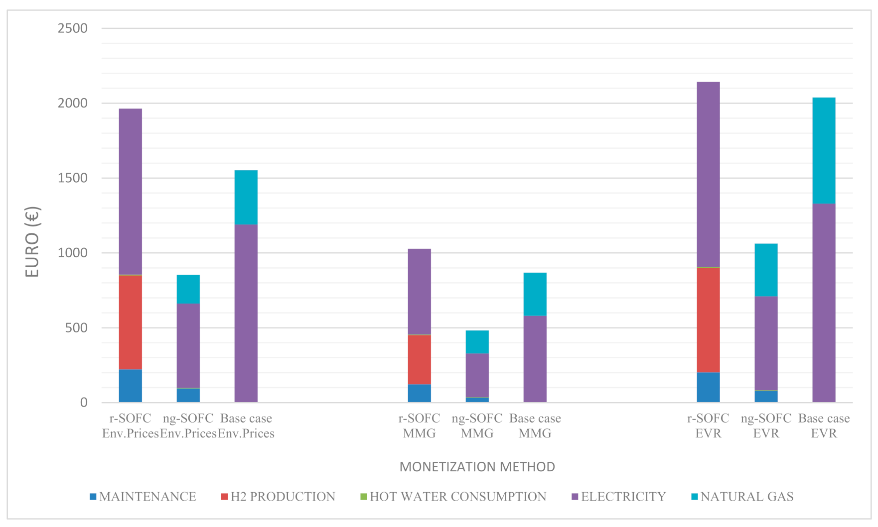
Results of the three different monetization methods are shown in Figure 7.

As can be seen in Figure 7, by all three methods the ng-SOFC is evaluated to have the lowest total environmental cost, followed by the base case scenario and the r-SOFC. The largest contribution to the environmental damage is given by electricity consumption in all the three scenarios, e.g., with Environmental Price method, 88% for the r-SOFC (electricity+H₂ production), 66% for the ng-SOFC and 77% for the Base case. Higher electricity consumption, for AC loads and appliances as well as for hydrogen production, and higher environmental impacts for maintenance phase determine the gap between the r-SOFC and the ng-SOFC. Of course, the ng-SOFC system makes use of natural gas, nevertheless the relative environmental cost is rather limited: 22% with Environmental Price, 32% with MMG and 33% with EVR. “MMG” results in lower total environmental costs than the “Environmental prices” method. The r-SOFC is still the most expensive alternative but the gap between one alternative and another is reduced by approximately a half.

According to the EVR method the ranking is confirmed. The ng-SOFC is the cheapest, followed by the base case and the r-SOFC. In this method, and to a smaller extent in MMG method too, the natural gas has a larger impact, leading to a greater contribution to the environmental cost for the ng-SOFC and the base case. As a consequence, with the EVR method the difference between the base case and the r-SOFC layout is the lowest among all the applied methods. Furthermore, the electricity is more impactful using this method that leads to raise the gap between the base case and the ng-SOFC, because the latter consumes a lower amount of energy overall.

In conclusion, the ranking between alternatives is the same using any of chosen monetization methods and, therefore, it can be considered a robust and reliable classification; differently, the single score values show a great variability.

For elaborating the idea of including a “corrective tax” in the energy bill, to adjust the private cost with the aim of incorporating the externalities, environmental costs have been added to other costs in the computation of the NPC. The environmental costs have been computed using the values obtained by the EVR monetization method because it presents the highest environmental costs.

The total impact is:

• 2142.75 €/year for the r-SOFC.
• 1062.47 €/year for the ng-SOFC.
• 2038.57 €/year in the base case scenario.

The introduction of a tax equal to the externalities modifies total saving of the systems as shown in Figure 8. The new total saving is computed as the difference between operational costs (energy cost + externalities) of the base case and operational costs (energy cost + externalities) of each fuel cell system over ten years.

When externalities are not considered (blue bars), the r-SOFC system results in negative total saving in the NM scenario and in the configuration i of SG incentive (i.e., there are not savings compared to the base case) while in configuration ii of SG incentive the total saving is 1685 EUR.

When externalities are included (orange bars) the total saving of the r-SOFC system reduces (796 EUR) because of its higher environmental costs than the base case.

On the contrary the total saving of the ng-SOFC is always positive and the best scenario is obtained using NM incentive. In this case the total saving is 9260 EUR, when externalities are not computed, and it increases by 89% (17,586 EUR) including externalities into the computation.

The analysis of these results shows that the inclusion of a tax equal to the environmental damage into the equation of NPC reduces the total saving of the r-SOFC system and increases total saving of the ng-SOFC.

An acceptable payback period (that should be at least equal to the lifetime of the investment) is obtained with a 50% C₀ reduction (or public contribution) for the ng-SOFC in the NM scenario with the inclusion of the tax on externalities.

4. Conclusions

This work aims at establishing the economic feasibility of two hybrid CHPs for residential application and, further, to evaluate the effectiveness of new Italian incentives for self-consumers’ groups and energy communities in reducing operational costs, when an energy storage technology is adopted (in the present case via hydrogen production by r-SOFC).

In order to fulfil the energy demand, two fuel cells (ng-SOFC and r-SOFC) are alternatively used and coupled with a PV system. Three different configurations have been analysed for each fuel cell: one concerning the net metering incentive and the others concerning the self-consumers’ group incentive. The economic feasibility of these systems is assessed, comparing them to a base case in which electric demand is provided by national grid and thermal demand is fulfilled by a natural gas boiler.

The results show that economic performance of the operational phase, i.e., without capital cost, obtains savings for the ng-SOFC, compared to the base case, in all the configurations.

On the contrary, the r-SOFC system leads to savings only when it is installed behind the meter and the SG incentive is applied.

Including capital cost, makes the resulting PBT to be much longer than the lifetime of the investment. This is in line with previous studies on these systems and highlights the needs of reducing costs of installation and purchase.

Comparison of the two incentives scenarios reveals that:

• The r-SOFC maximizes its economic performance when the self-consumers’ incentive (SG) is applied.
• The ng-SOFC maximizes its economic performance when the net metering incentive (NM) is applied.

The r-SOFC layout essentially includes an energy storage system, that allows to raise the use of solar energy and maximize self-consumption. Such management of renewable energy is coherent with the scope of the SG incentives and, therefore, is rewarded by the incentive scheme. On the other hand, the ng-SOFC system produces electrical energy, using fossil fuel, and its economic performance is maximized in a scheme which encourages energy production, like NM. Although SG incentives make the adoption of r-SOFC profitable, a layout consisting of ng-SOFC still remains the most advantageous.

With respect to externalities, we analyse variations of annual savings by the introduction of a tax (equal to the environmental impact) on the price of the systems aimed at driving the market towards green solutions. The monetization of externalities by means of three different methods shows that the environmental cost of the ng-SOFC system is the lowest among the alternatives, followed by the base case and at last, the r-SOFC system. This leads to an increase of the annual savings of the ng-SOFC system by about 50% each year. The ng-SOFC system would be incentivized by the internalization of environmental costs into direct costs. The r-SOFC system in this case results in higher environmental costs than the base case.

Moreover, the sensitivity analysis shows that the energy prices are not critical variables not significantly affecting the results. Thereafter, the general results of this paper can be extended also to different energy markets beyond the Italian one.

Based on the present study of a hybrid m-CHP, economic analysis, incentives evaluation and externalities assessment point to the conclusion that grey hydrogen (ng-SOFC) still remains a more competitive technology than a not-fully-green hydrogen (r-SOFC).

In general, hydrogen and fuel cell technologies currently have a good level of maturity but to become competitive for commercial purposes they need investments that offer long-term stability, necessary to carry out large deployments. Such initiatives (governmental incentives, research investment etc.) may lead hydrogen and fuel cells to achieve better costs and performances, as it has been done in the case of technologies such solar photovoltaics. In the future, fuel cell technologies, when properly supported, may represent a complementary low-carbon alternative to be used in multiple applications throughout the energy system. In authors’ opinion, some technological development may improve economic and environmental performances of r-SOFC systems. For example, a higher round trip efficiency would lower the total energy demand of the system; a smarter switch between fuel cell mode and electrolyser mode (e.g., programming electrolyser time window with weather forecast) would lower the amount of energy taken out from the grid. However, different storage systems can benefit from SG incentives scheme more efficiently than the studied r-SOFC system and, this case study demonstrates how effectively SG incentives can favour the birth of self-consumers’ groups and energy communities

References

1. Organization of the Petroleum Exporting Countries. 2017 OPEC World Oil Outlook. October 2017. Available online: http://www.opec.org (accessed on 1 July 2021).
2. World-Energy-Outlook-2020. Available online: https://www.iea.org/reports/world-energy-outlook-2020 (accessed on 1 July 2021).
3. IEO. 2019. Available online: https://www.eia.gov/outlooks/ieo/pdf/ieo2019.pdf (accessed on 1 July 2021).
4. Sui, S.; Rasheed, R.; Li, Q.; Su, Y.; Riffat, S. Techno-economic modelling and environmental assessment of a modern PEMFC CHP system: A case study of an eco-house at University of Nottingham. Environl. Sci. Poll. Res. 2019, 26, 29883–29895. [Google Scholar] [CrossRef] [PubMed]
5. IEA. Tracking Buildings. 2020. Available online: https://www.iea.org/reports/tracking-buildings-2020 (accessed on 1 July 2021).
6. Jing, R.; Wang, M.; Wang, W.; Brandon, N.; Li, N.; Chen, J.; Zhao, Y. Economic and environmental multi-optimal design and dispatch of solid oxide fuel cell based CHP systems. Energy Convers. Manag. 2017, 154, 365–379. [Google Scholar] [CrossRef]
7. Strazza, C.; Del Borghi, A.; Costamagna, P.; Gallo, M.; Brignole, E.; Girdinio, P. Life Cycle Assessment and Life Cycle Costing of a SOFC system for distributed power generation. Energy Convers. Manag. 2015, 100, 64–77. [Google Scholar] [CrossRef]
8. Nielsen, E.R.; Prag, C.B.; Bachmann, T.M.; Carnicelli, F.; Boyd, E.; Walker, I.; Ruf, L.; Stephens, A. Status on Demonstration of Fuel Cell Based Micro-CHP Units in Europe. Fuel Cells 2019, 19, 340–345. [Google Scholar] [CrossRef]
9. Gomez, S.Y.; Hotza, D. Current developments in solid oxide fuel cells. Renew. Sust. Ener. Rev. 2016, 61, 155–174. [Google Scholar] [CrossRef]
10. Barelli, L.; Bidini, G.; Cinti, G.; Ottaviano, A. Study of SOFC-SOE transition on a RSOFC stack. Int. J. Hydrog. Energy 2017, 42, 26037–26047. [Google Scholar] [CrossRef]
11. Mendoza, R.M.; Mora, J.M.; Cervera, R.B.; Chuang, P.Y.A. Experimental and Analytical Study of an Anode-Supported Solid Oxide Electrolysis Cell. Chem. Eng. Technol. 2020, 43, 2350–2358. [Google Scholar] [CrossRef]
12. Almaraz, S.D.L.; Azzaro-Pantel, C. Design and optimization of hydrogen supply chains for a sustainable future. Hydrog. Econ. 2017, 85–120. [Google Scholar] [CrossRef]
13. Hydrogen for Europe-SRIA Clean Hydrogen for Europe—Final Draft—Strategic Research and Innovation Agenda—July 2020. Available online: https://www.hydrogeneurope.eu/wp-content/uploads/2021/04/20201027-SRIA-CHE-final-draft-1.pdf (accessed on 20 March 2021).
14. Di Florio, G.; Macchi, E.G.; Mongibello, L.; Baratto, M.C.; Basosi, R.; Busi, E.; Caliano, M.; Cigolotti, C.; Testi, M.; Trini, M. Comparative life cycle assessment of two different SOFC-based cogeneration systems with thermal energy storage integrated into a single-family house nanogrid. Appl. Energy 2021, 285, 116378–116398. [Google Scholar] [CrossRef]
15. Pellegrino, S.; Lanzini, A.; Leone, P. Techno-economic and policy requirements for the market-entry of the fuel cell micro-CHP system in the residential sector. Appl. Energy 2015, 143, 370–382. [Google Scholar] [CrossRef]
16. Rossi, F.; Heleno, M.; Basosi, R.; Sinicropi, A. LCA driven solar compensation mechanism for Renewable Energy Communities: The Italian case. Energy 2021, 235, 121374. [Google Scholar] [CrossRef]
17. Poponi, D.; Basosi, R.; Kurdgelashvili, L. Subsidisation cost analysis of renewable energy deployment: A case study on the Italian feed-in tariff programme for photovoltaics. Energy Policy 2021, 154, 112297. [Google Scholar] [CrossRef]
18. Elmer, T.; Worall, M.; Wu, S.; Riffat, S.B. Emission and economic performance assessment of a solid oxide fuel cell micro-combined heat and power system in a domestic building. Appl. Therm. Eng. 2015, 90, 1082–1089. [Google Scholar] [CrossRef]
19. Rogers, J.G.; Cooper, S.J.G.; O’Grady, Á.; McManus, M.C.; Howard, H.R.; Hammond, G.P. The 20% house—An integrated assessment of options for reducing net carbon emissions from existing UK houses. Appl. Energy 2015, 138, 108–120. [Google Scholar] [CrossRef] [Green Version]
20. Facci, A.L.; Cigolotti, V.; Jannelli, E.; Ubertini, S. Technical and economic assessment of a SOFC-based energy system for combined cooling, heating and power. Appl. Energy 2017, 192, 563–574. [Google Scholar] [CrossRef]
21. Mubaarak, S.; Zhang, D.; Chen, Y.; Liu, J.; Wang, L.; Yuan, R.; Wu, J.; Zhang, Y.; Li, M. Techno-Economic Analysis of Grid-Connected PV and Fuel Cell Hybrid System Using Different PV Tracking Techniques. Appl. Sci. 2020, 10, 8515. [Google Scholar] [CrossRef]
22. Tazay, A. Techno-Economic Feasibility Analysis of a Hybrid Renewable Energy Supply Options for University Buildings in Saudi Arabia. Open Eng. 2021, 11, 39–55. [Google Scholar] [CrossRef]
23. Gharibi, M.; Askarzadeh, A. Size and power exchange optimization of a grid connected diesel generator-photovoltaic-fuel cell hybrid energy system considering reliability, cost and renewability. Int. J. Hydrog. Energy 2019, 44, 25428–25441. [Google Scholar] [CrossRef]
24. Zhang, Y.; Campana, P.E.; Lundblad, A.; Yan, J. Comparative study of hydrogen storage and battery storage in grid connected photovoltaic systems: Storage sizing and rule-based operation. Appl. Energy 2017, 201, 397–411. [Google Scholar] [CrossRef]
25. Sedaghati, R.; Shakarami, M.R. A novel control strategy and power management of hybrid PV/FC/SC/battery renewable power system-based grid-connected microgrid. Sustain. Cities Soc. 2019, 44, 830–843. [Google Scholar] [CrossRef]
26. Abdelshafy, A.M.; Hassan, H.; Jurasz, J. Optimal design of a grid-connected desalination plant powered by renewable energy resources using a hybrid PSO–GWO approach. Energy Convers. Manag. 2018, 173, 331–347. [Google Scholar] [CrossRef]
27. Lamagna, M.; Nastasi, B.; Groppi, D.; Rozain, C.; Manfren, M.; Garcia, D.A. Techno-economic assessment of reversible Solid Oxide Cell integration to renewable energy systems at building and district scale. Energy Convers. Manag. 2021, 235, 113993. [Google Scholar] [CrossRef]
28. Monforti Ferrario, A.; Vivas, F.J.; Segura Manzano, F.; Andújar, J.M.; Bocci, E.; Martirano, L. Hydrogen vs. battery in the long-term operation. A comparative between energy management strategies for hybrid renewable microgrids. Electronics 2020, 9, 698. [Google Scholar] [CrossRef]
29. Krishan, O.; Suhag, S. Techno-economic analysis of a hybrid renewable energy system for an energy poor rural community. J. Energy Storage 2019, 23, 305–319. [Google Scholar] [CrossRef]
30. Singh, A.; Baredar, P.; Gupta, B. Techno-economic feasibility analysis of hydrogen fuel cell and solar photovoltaic hybrid renewable energy system for academic research building. Energy Convers. Manag. 2017, 145, 398–414. [Google Scholar] [CrossRef]
31. Fazelpour, F.; Soltani, N.; Rosen, M.A. Economic analysis of standalone hybrid energy systems for application in Tehran, Iran. Int. J. Hydrog. Energy 2016, 41, 7732–7743. [Google Scholar] [CrossRef]
32. Duman, A.C.; Güler, Ö. Techno-economic analysis of off-grid PV/wind/fuel cell hybrid system combinations with a comparison of regularly and seasonally occupied households. Sustain. Cities Soc. 2018, 42, 107–126. [Google Scholar] [CrossRef]
33. Sorace, M.; Gandiglio, M.; Santarelli, M. Modeling and techno-economic analysis of the integration of a FC based micro-CHP system for residential application with a heat pump. Energy 2017, 120, 262–275. [Google Scholar] [CrossRef]
34. Martinoupolous, G. Are rooftop photovoltaic systems a sustainable solution for Europe? A life cycle impact assessment and cost analysis. Appl. Energy 2020, 257, 114035. [Google Scholar] [CrossRef]
35. Fu, R.; Feldman, D.J.; Margolis, R.M. US Solar Photovoltaic System Cost Benchmark: Q1 2018; No. NREL/TP-6A20-72399; National Renewable Energy Lab (NREL): Golden, CO, USA, 2018. [Google Scholar]
36. Rad, M.A.V.; Ghasempour, R.; Rahdan, P.; Mousavi, S.; Arastounia, M. Techno-economic analysis of a hybrid power system based on the cost-effective hydrogen production method for rural electrification, a case study in Iran. Energy 2020, 190, 116421. [Google Scholar] [CrossRef]
37. Rossi, F.; Heleno, M.; Basosi, R.; Sinicropi, A. Environmental and economic optima of solar home systems design: A combined LCA and LCC approach. Sci. Total Environ. 2020, 744, 140569–140580. [Google Scholar] [CrossRef] [PubMed]
38. ARERA. Condizioni Economiche per i Clienti del Mercato Tutelato. Available online: https://www.arera.it/it/dati/condec.htm (accessed on 27 January 2021).
39. Kuckshinrichs, W.; Koj, J.C. Levelized cost of energy from private and social perspectives: The case of improved alkaline water electrolysis. J. Clean. Prod. 2018, 203, 619–632. [Google Scholar] [CrossRef]
40. Capros, P.; De Vita, A.; Tasios, N.; Siskos, P.; Kannavou, M.; Petropoulos, A.; Evangelopoulou, S.; Zampara, M.; Papadopoulos, D.; Paroussos, L.; et al. EU Energy, Transport and GHG Emissions. Trends to 2050; Directorate-General for Energy, Directorate-General for Climate Action and Directorate-General for Mobility and Transport; Publications Office of the European Union: Luxemburg, 2016; Available online: http://pure.iiasa.ac.at/id/eprint/13656/1/REF2016_report_FINAL-web.pdf (accessed on 19 March 2021).
41. RSE Colloquia. Decarbonizzazione Dell’economia Italiana Scenari di Sviluppo del Sistema Energetico Nazionale IV Volume 2017 Presso Arti Grafiche Fiorin SPA Via del Tecchione 36|20098 Sesto Ulteriano|San Giuliano Milanese (MI) Prima edizione, 130-13. ISBN 978-88-907527-6-6. Available online: https://www.mite.gov.it/sites/default/files/archivio/allegati/rse_decarbonizzazione_web.pdf (accessed on 16 March 2021).
42. ARERA. Autorità di Regolazione per Energia Reti ed Ambiente-Deliberazione 4 agosto 2020 318/2020/R/EEL “Regolazione delle Partite Economiche Relative all’Energia Elettrica Condivisa da un Gruppo di Aut-consumatori di Energia Rinnovabile che Agiscono Collettivamente in Edifici e Condomini oppure Condivisa in una Comunità di Energia Rinnovabile”. Available online: https://www.arera.it/allegati/docs/20/318-20.pdf (accessed on 10 May 2021).
43. D.LGS 30 December 2019; n. 162. Available online: https://www.gazzettaufficiale.it/eli/id/2019/12/31/19G00171/sg (accessed on 7 May 2021).
44. Renewable Energy Directive 2018/2001/EU (REDII). Available online: https://eur-lex.europa.eu/legal-cotent/EN/TXT/?uri=CELEX%3A32018L2001 (accessed on 6 April 2021).
45. Kostas, B. Sustainability and externalities: Is the internalization of externalities a sufficient condition for sustainability? Ecol. Econ. 2011, 70, 1703–1706. [Google Scholar]
46. United Nations Environment Programme. Universal Ownership—Why Environmental Externalities Matter to Institutional Investors; PRI Association and UNEP Finance Initiative: Nairobi, Kenya, 2011. [Google Scholar]
47. Stiglitz, J.E. The Economics of the Public Sector, 3rd ed.; W.W. Norton: New York, NY, USA, 2000; Available online: http://go.owu.edu/rjgitter/Six%20Market%20Failures.pdf (accessed on 26 April 2021).
48. Cornes, R.; Sandler, T. The Theory of Externalities, Public Goods, and ClubGoods; Cambridge University Press: New York, NY, USA, 1996. [Google Scholar]
49. Nguyen, T.L.T.; Laratte, B.; Guillaume, B.; Hua, A. Quantifying environmental externalities with a view to internalizing them in the price of products, using different monetization models. Resour. Conserv. Recycl. 2016, 109, 13–23. [Google Scholar] [CrossRef]
50. Corona, B.; Cerrajero, E.; López, D.; San Miguel, G. Full environmental life cycle cost analysis of concentrating solar power technology: Contribution of externalities to overall energy costs. Solar Energy 2016, 135, 758–768. [Google Scholar] [CrossRef]
51. Arendt, R.; Bachmann, T.M.; Motoshita, M.; Bach, V.; Finkbeiner, M. Comparison of Different Monetization Methods in LCA: A Review. Sustainability 2020, 12, 10493–10532. [Google Scholar] [CrossRef]
52. Speck, S. Overview of Environmental Tax Reforms in EU Member States, National Environmental Research Institute/University of Aarhus, Denmark, Project. Package 1 of the Final Report of the COMETR. 2007. Available online: http://www2.dmu.dk/cometr/COMETRFinalReport.pdf (accessed on 20 April 2021).
53. Prud’homme, R. Marginal social cost pricing in transport policy. In Proceedings of the Discussion Paper Presented at the 7th ACEA SAG Meeting on “Marginal Social Cost Pricing in Transport Policy”, Brussels, Belgium, 18 September 2001. [Google Scholar]
54. Soliwoda, M.; Pawłowska-Tyszko, J. Tax Policy Tools vs. Sustainable Development of Agriculture—The Case of Poland. In Proceedings of the 17th International Academic Conference of the International Institute of Social and Economic Sciences, Vienna, Austria, 21 June 2015. [Google Scholar]
55. Vogtländer, J.G.; Brezet, H.C.; Hendriks, C.F. The virtual eco-costs ‘99 A single LCA-based indicator for sustainability and the eco-costs-value ratio (EVR) model for economic allocation. Int. J. Life Cycle Assess. 2001, 6, 157–166. [Google Scholar] [CrossRef]
56. De Bruyn, S.; Bijleveld, M.; de Graaff, L.; Schep, E.; Schroten, A.; Vergeer, R.; Ahdour, S. Environmental Prices Handbook; CE Delft: Delft, The Netherlands, 2018. [Google Scholar]
57. MMG Annex: Monetisation of the MMG method (update 2017). Available online: http://www.ovam.be (accessed on 6 February 2021).
58. Florio, M.; Finzi, U.; Genco, M.; Levalert, F.; Mafii, S.; Tracogna, A.; Vignetti, S. Analisi di sensibilità e di rischio. In Guida All’analisi Costi-Benefici dei Progetti di Investimento; Unità di Valutazione, DG Politica Regionale e Coesione; Commissione Europea: Brussels, Belgium, 2003; Available online: https://ec.europa.eu/regional_policy/sources/docgener/guides/cost/guide02_it.pdf (accessed on 30 March 2021).
Figure 1. (A) Configuration with the fuel cells in front of the meter (i–iii). (B) Configuration installing the fuel cell behind the meter (ii–iv).
Energies 14 05847 g001
Figure 2. Costs and incentives of the systems in the “net metering” scenario.
Energies 14 05847 g002
Figure 3. Costs and incentives of the systems in the self-consumers group scenarios.
Energies 14 05847 g003
Figure 4. Normalised “operational phase” NPC values in each scenario.
Energies 14 05847 g004
Figure 5. Sensitivity analysis (NM) with ±5% variations of energy price. PEE: price of electricity.PNG: price of natural gas. Both: price of electricity and price of natural gas.
Energies 14 05847 g005
Figure 6. Sensitivity analysis (SG) with ±5% variations of energy price. PEE: price of electricity. PNG: price of natural gas. Both: price of electricity and price of natural gas.
Energies 14 05847 g006
Figure 7. Total environmental costs for each method.
Energies 14 05847 g007
Figure 8. Comparison of total saving with and without externalities in the different incentive scenarios.
Energies 14 05847 g008