Transmission Network Expansion Planning Considering Wind Power and Load Uncertainties Based on Multi-Agent DDQN

Abstract

This paper presents a multi-agent Double Deep Q Network (DDQN) based on deep reinforcement learning for solving the transmission network expansion planning (TNEP) of a high-penetration renewable energy source (RES) system considering uncertainty. First, a K-means algorithm that enhances the extraction quality of variable wind and load power uncertain characteristics is proposed. Its clustering objective function considers the cumulation and change rate of operation data. Then, based on the typical scenarios, we build a bi-level TNEP model that includes comprehensive cost, electrical betweenness, wind curtailment and load shedding to evaluate the stability and economy of the network. Finally, we propose a multi-agent DDQN that predicts the construction value of each line through interaction with the TNEP model, and then optimizes the line construction sequence. This training mechanism is more traceable and interpretable than the heuristic-based methods. Simultaneously, the experience reuse characteristic of multi-agent DDQN can be implemented in multi-scenario TNEP tasks without repeated training. Simulation results obtained in the modified IEEE 24-bus system and New England 39-bus system verify the effectiveness of the proposed method.

1. Introduction

Although countries have actively implemented Nationally Determined Contributions (NDCs) to alleviate climate deterioration in recent years, global greenhouse gas emissions are still in the process of continuous growth, and there has not yet been a peak phenomenon. In order to control the future temperature rise within 1.5 °C, the United Nations Environment Programme advocates that countries around the world should reduce the emissions to fill the gap between the current greenhouse gas emissions level and the Paris Agreement provisions [1]. The transformation of energy structure is regarded as the primary way for emissions reduction by all countries. Many countries have formulated plans to build a high-penetration renewable energy source (RES) system, which fully releases the high environmental and economic value of renewable energy by replacing fossil energy [2,3]. There are two main challenges in the RES system construction. One is to solve the time and space uncertainties caused by the intermittency of renewable energy [4], and the other is to optimize the network structure for large-scale renewable energy integration [5]. The transmission network expansion planning (TNEP) is the crucial task of power system construction, which determines the basic structure and system characteristic. Therefore, the characteristics of system with high-penetration of RES should be fully considered in the TNEP task on the basis of ensuring system stability and economy.

In a high-penetration RES system, as general generators are gradually replaced by renewable energy, the increase in the penetration rate of renewable energy makes the system operation state more diversified [6,7], and the uncertainties of the load-side and the source-side are also amplified. The TNEP task of a high-penetration RES system should first obtain the description of the renewable energy uncertainty. The uncertainty description is mainly obtained through the scenario generation method based on probabilistic power flow and the representative days method based on system operating data. The scenario generation method does not require a large amount of operation data. It abstracts the characteristics of renewable energy and variable load fluctuations, and appropriately estimates operation data according to task requirements. In reference [8], the uncertainty of renewable energy and demand resources (DR) was decomposed by robust optimization theory according to the robust intervals on multiple timescales, and the modeling method was selected in conformity with the characteristics of each component to form the uncertain model. Furthermore, the relationship between DR and RES was considered in uncertain model to form a multi-energy hub in [9]. References [9,10] established a model based on the uncertain characteristics of renewable energy, and studied the electricity market trading strategy of the RES system. The scenario generation method is intuitive and practical, which can greatly speed up the problem-solving. However, the accuracy of the uncertainty description of regional equipment is extremely important in the TNEP tasks [11]. Therefore, more and more studies have turned to constructing uncertain models from operation data. Reference [12] studied the relationship between the system’s renewable energy penetration rate and typical operating conditions based on a data-driven method, and verified that when the penetration rate increases from 20% to 40%, the system typical states will increase 4 times. Reference [13] improved the K-Means algorithm by taking the maximum and minimum output of renewable energy as the classification condition, and the classified representative days data is more in line with the needs of the TNEP task. In addition, the duration curve of renewable energy was also used to generate the uncertain model, and the multiple typical scenario duration curves were generated according to seasons, times, weather conditions and demand levels in reference [14]. Therefore, this paper will use the system operation data to construct the uncertain model of renewable energy and variable load to assist the TNEP task solving, and use the data compression method to maintain the efficiency of the calculation while retaining the main characteristics of the uncertain model.

The huge uncertainties of the source-side and the load-side in the system with high-penetration of RES make the power shortage more frequent [15]. The transmission stability in a wide area cannot be maintained only by the local balance of power generation and load. It is also necessary to build a more compact transmission network structure through TNEP task to release the potential of power support among various renewable energy sources [16]. The construction of the TNEP model of the system with high-penetration of RES should fully consider the uncertain characteristics of renewable energy and variable loads, and improve the stability of system in the most economical way. Reference [17] proposed a two-stage model of TNEP and the renewable energy generation expansion planning (REGEP), which can coordinate system stability and renewable energy consumption in complex situations. On this basis, the system outages and post-contingency control were added to construct a five-level model in reference [18]. For some special scenarios, environmental conditions are also used as part of the TNEP model to assist decision-making. For example, reference [19] constructed an offshore grid planning model based on the typical connection structure of offshore wind farms. The comprehensive TNEP model can ensure that the planning scheme meets the various requirements of network construction. The solution of traditional TNEP model is a complex and large-scale mixed-integer linear programming (MILP) problem [18], and many studies have focused on improving the solution efficiency. The Benders decomposition method was adopted to reduce the complexity of model in references [20,21]. Furthermore, combining Benders decomposition method with the Column-and-Constraint generation method, reference [22] proposed a better method to obtain the planning scheme with high reliability and economy for RES system. In addition, the primal cutting planes algorithm was also used to accelerate the TNEP solution in reference [23]. With the increase in the scale of the system with high-penetration of RES and the nonlinear constraints of the TNEP model, the traditional decomposition method has encountered a bottleneck, which makes the heuristic-learning based method a more convenient way to obtain planning scheme. Reference [24] used the improved Particle Swarm Optimization (PSO) to solve the multi-objective TNEP model, which contains the security and uncertain constraints of photovoltaic power farms. Reference [25] separated the cost problem from the investment problem in TNEP model, and solved them by PSO and quadratic programming (QP) methods, respectively. In addition, under the uncertain scenario, the shuffled frog leaping algorithm (SFLA) was adopted to process the TNEP task, which obtained a better scheme than PSO in reference [26]. Although the heuristic learning-based method can solve TNEP problem more quickly than decomposition methods, the black box characteristic of such methods makes the solution process interpretability extremely low. At the same time, it requires thorough retraining for different tasks, which wastes time. Deep reinforcement learning is currently an advanced technology, and it is widely used in power system load frequency contortion, flow adjustment, and AGC power order optimization in references [27,28,29]. However, the application of deep reinforcement learning to the TNEP tasks is still in the early stage. Reference [30] adopted Deep Q Network (DQN) to solve the TNEP model based on the static system. Nevertheless, when undertaking the TNEP tasks for the system with high-penetration of RES, the deep reinforcement learning environment should contain more uncertain characters of wind power and variable load. Moreover, the reinforcement learning structure should be redesigned accordingly to satisfy more complex model solving.

The contributions of this paper are listed below:

• A K-means algorithm that enhances the extraction quality of variable wind and load power uncertain characteristics is proposed. The proposed method considers the accumulation and change rate of operational data.
• A calculation method of wind curtailment and load shedding that reduces the computational complexity while retaining the uncertainty of the system is proposed. The calculation method is based on the typical uncertain scenarios extracted from operation data.
• A TNEP bi-level model considering the system stability and economy is constructed, and this model includes the comprehensive cost, wind curtailment, load shedding, and electrical betweenness.
• Multi-agent DDQN is proposed based on the bi-level model, which is a high-performance and interpretable machine learning method for the TNEP task.

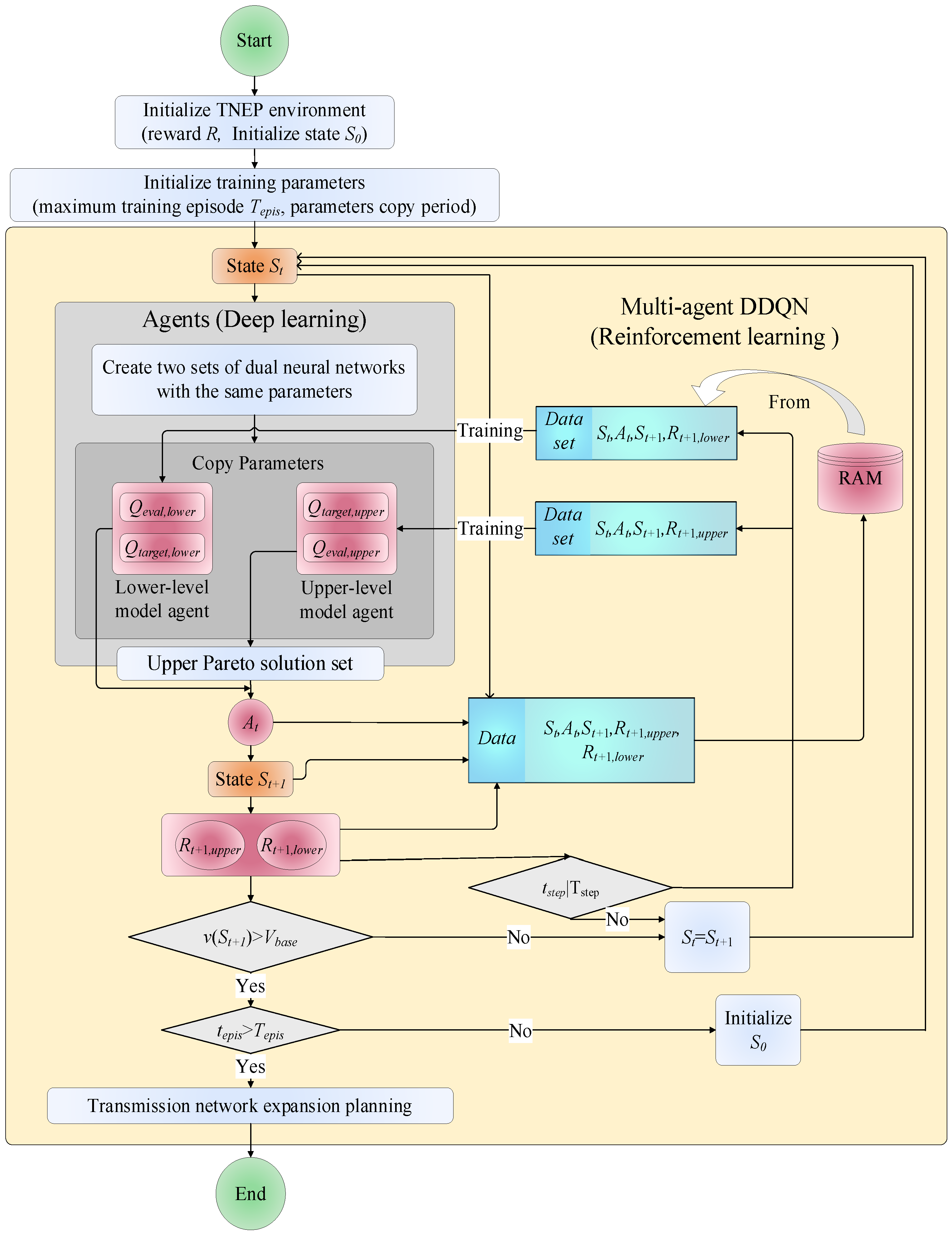
This paper is organized as follows: Section 2 constructs the bi-level TNEP model to consider the wind power and load uncertainties. Section 3 builds the multi-agent DDQN for TNEP task based on deep reinforcement learning. Section 4 takes multi-agent DDQN to complete TNEP tasks on modified IEEE 24-bus system and New England 39-bus system.

2. TNEP Bi-Level Model Based on Typical Scenarios of Wind Power and Load Uncertainties

This section constructs a TNEP bi-level model considering the system stability and economy based on uncertain scenarios. First, the typical uncertain scenarios of wind power and load data are extracted based on the improved K-Means algorithm. Secondly, based on the extracted results, a TNEP bi-level model is constructed. This model can comprehensively evaluate the economic and stability of transmission network under the scenario of a high-penetration of wind power and variable load.

2.1. Improved K-Means Algorithm Based on Characteristics of Wind power and Load Operation Data

The output power of a wind farm is closely related to the regional weather, and the load-side behavior also makes the input power of the load variable. The system with high-penetration wind farms and variable load injection face high uncertainties at the source-side and load-side, which greatly affects the stability of the RES system. In the system to be expanded, there are many combinations of wind farm output power and load input power recorded in historical operating data, and it is unrealistic to consider each scenario in the TNEP task. Therefore, this paper uses the improved K-Means algorithm to extract typical scenarios, which saves a lot of calculation time for TNEP task while preserving the system uncertainty.

K-Means algorithm is an intuitive and efficient clustering method based on the distance of data samples. Additionally, when applied to the classification task of large data sets, its performance is still excellent.

When the K-Means algorithm is used to extract typical scenarios from operating data, the K value should be given first to determine K cluster centers. Then, through iterative optimization of K cluster centers, the sum of the distances between the classified samples and each cluster center is minimized. The traditional sum of the squared errors (SSE) is

$$SSE={{\displaystyle {\sum }_{n=1}^K{\displaystyle {\sum }_{x\in \delta }(x-C_n)}}}^2,$$

(1)

where x is the operation data; δ is the operation data set; C_n is data of cluster center.

However, when traditional SSE is used for clustering task, its morphological-based clustering objective cannot fully reflect the fluctuation characteristics and accumulation of operation data, which are quite critical for the TNEP task. Therefore, this paper proposes to adopt accumulation and change rate as indicators to measure the data uncertainty, and then use these two indicators as clustering objective to improve the quality of clustering data.

The cumulation of operation data D_cumulative is

$$D_{cumulative}={\displaystyle {\sum }_{h=1}^{24}{d}_h}$$

(2)

where d_h is value of operation data at h-th hour, and the change rate of operation data D_change is

$$D_{change}={\displaystyle {\sum }_{h=2}^{24}(d_h-d_{h-1})}/d_{rated}$$

(3)

where d_rated is the rated value of operation data; d_h−1 is value of operation data at h − 1-th hour.

Based on (2) and (3), the clustering objective function SSE_new of improved K-Means algorithm is

$$SS{E}_{new}={{\displaystyle {\sum }_{n=1}^K{\displaystyle {\sum }_{x\in \delta }[(D_{cumulative,x}-C_{cumulative,n})}}}^2+{(D_{change,x}-C_{change,n})}^2].$$

(4)

where D_cumulative,x is the cumulation of operation data x; C_cumulative,n is the cumulation of clustering center n; D_change,x is the change rate of operation data x; C_change,n is the change rate of clustering center n.

2.2. Bi-Level Multi-Objective TNEP Model

The TNEP task of the RES system is a multi-objective problem. It needs to coordinate economy and stability. In addition, the uncertainties of the system under large-scale wind power and variable load should also be considered. Therefore, this section constructs a bi-level model based on the nature of the transmission network evaluation index, and each layer model is composed of objective function and constraints.

2.2.1. Upper-Level Objective Function

The upper-level model uses the comprehensive cost to evaluate the economy of the system. The comprehensive cost is composed of construction cost, network loss cost, and operation and maintenance cost. The construction cost f₁ of the TNEP task is formed by the uniform annual investment of transmission lines.

$$f_1=\frac{r_d{(1+r_d)}^y}{{(1+r_d)}^y-1}{\displaystyle {\sum }_{l=1}^{N_L}{\lambda }_l{X}_l},$$

(5)

where r_d is the capital discount rate of line; y is the life expectancy of line; N_L is the total number of lines; λ_l is the line construction state; X_l is the construction investment of line l.

The transmission network loss refers to the power loss in the form of heat energy during the power transmission, the transmission network loss cost f₂ is

$$f_2=p_{loss}{\displaystyle {\sum }_{l=1}^{N_L}\frac{P_l^2+Q_l^2}{U_l^2}{r}_l},$$

(6)

where P_l is the active power of line l in AC rectangular; Q_l is the active power of line l in AC rectangular; U_l is the voltage of line l in AC rectangular; p_loss is the unit electricity price of network loss.

The operation and maintenance cost of the transmission network should consider the equipment of line and transformer. However, the transformer operation and maintenance cost is related to the load rate, and the parameters and transmission power of each transformer in the IEEE RTS-24 bus system are almost equal. Therefore, the transformer operation and maintenance cost have little effect on the scheme choice. The system operation and maintenance cost f₃ is

$$f_3={\displaystyle {\sum }_{l=1}^{N_L}{\eta }_l{\lambda }_l{X}_l},$$

(7)

where η_l is the line operation and maintenance cost coefficient.

The calculation of upper-level objective function is based on the AC power flow method, which can describe power flow characteristics more accurately than the DC power flow method used in traditional TNEP methods. The f_upper(·) is

$$f_{upper}(\cdot )=\min {\left[f_1(l),f_2(l),f_3(l)\right]}^T.$$

(8)

2.2.2. Upper-Level Constraints

The upper-level constraints are mainly composed of power transmission and equipment operation constraints. The AC power flow balance constraints are

$$P_j^g-P_{wind,j}^{curt}-V_j{\displaystyle {\sum }_{k\in j}(G_{jk}\cos {\theta }_{jk}+B_{jk}\sin {\theta }_{jk})=}{P}_j^{load}-P_{load,j}^{shed},$$

(9)

$$Q_j^g-Q_{wind,j}^{curt}-V_j{\displaystyle {\sum }_{k\in j}(G_{jk}\sin {\theta }_{jk}+B_{jk}\cos {\theta }_{jk})=}{Q}_j^{load}-Q_{load,j}^{shed}-Q_j^c,$$

(10)

where $P_j^g$ is the generator rated active power output of node j; $P_{wind,j}^{curt}$ is the wind curtailment active power of node j; V_j is the voltage of node j; B_jk is the susceptance between node j and node k; G is the conductivity between node j and node k; θ_jk is the phase angle between node j and node k; $P_j^{load}$ is the load active power input of node j; $P_{load,j}^{shed}$ is the load active power shedding of node j; $Q_j^g$ is the generator reactive power output of node j; $Q_j^{load}$ is the reactive power input of node j; $Q_{wind,j}^{curt}$ is the wind curtailment reactive power of node j; $Q_{load,j}^{shed}$ is the load reactive power of node j; $Q_j^c$ is the reactive power of reactive power compensation device of node j.

The voltage amplitude and phase angle constraints are

$$V_j^{\min ,upper}\le V_j\le V_j^{\max ,upper},$$

(11)

$${\theta }_j^{\min ,upper}\le {\theta }_j\le {\theta }_j^{\max ,upper},$$

(12)

where $V_j^{\min ,upper}$ and $V_j^{\max ,upper}$ are the maximum and minimum of voltage of node j; ${\theta }_j^{\min ,upper}$ and ${\theta }_j^{\max ,upper}$ are the maximum and minimum of phase angle of node j.

Because wind farm has strong reactive power regulation capability, this paper does not make a special constraint. The wind power and general generator output constraints are

$$P_j^{g,\min }\le P_j^g\le P_j^{g,\max },$$

(13)

$$P_j^{wind,\min }\le P_j^{wind}\le P_j^{wind,\max },$$

(14)

$$Q_j^{g,\min }\le Q_j^g\le Q_j^{g,\max },$$

(15)

where $P_j^{g,\max }$ and $P_j^{g,\min }$ are the maximum and minimum of generator active power output; $Q_j^{g,\max }$ and $Q_j^{g,\min }$ is the maximum and minimum of generator reactive power output; $P_j^{wind,\max }$ and $P_j^{wind,\min }$ is the maximum and minimum of wind active power output.

The line transmission capacity constraint is

$$-F_l^{\max }\le F_l\le F_l^{\max },$$

(16)

where the F_l is the power flow of line l; $F_l^{\max }$ is the power flow transmission maximum line j.

The wind curtailment constraint is

$$0\le P_{wind,j}^{curt}\le \min ({\mu }_j^{wind}{P}_j^{wind},P_{wind,j}^{curt,lower}),$$

(17)

where μ_wind,j is the minimum output ratio; $P_{wind,j}^{curt,lower}$ is the wind active power curtailment of lower-level model.

The load shedding constraint is

$$0\le P_{load,j}^{shed}\le \min ({\mu }_j^{load}{P}_j^{load},P_{load,j}^{shed,lower}),$$

(18)

where μ_load,j is the minimum load ratio; $P_{load,j}^{shed,lower}$ is the load activate power shedding of lower-level model; $P_{wind,j}^{curt,lower}$ is the wind active power curtailment of lower-level model.

2.2.3. Lower-Level Objective Function

The lower-level model is based on typical uncertain scenarios. It evaluates renewable energy consumption of system through load shedding and wind curtailment calculations, and the system stability is evaluated by the improved electrical betweenness. Based on the bi-level model structure, the upper-level model obtains a Pareto set composed of better economical lines, and the lower-level model only needs to calculate the scheme in this set. Then, the upper-level model further optimizes the TNEP scheme after receiving the calculation results of lower-level model. This mechanism satisfies the constraints between the bi-level models and improves the computational efficiency.

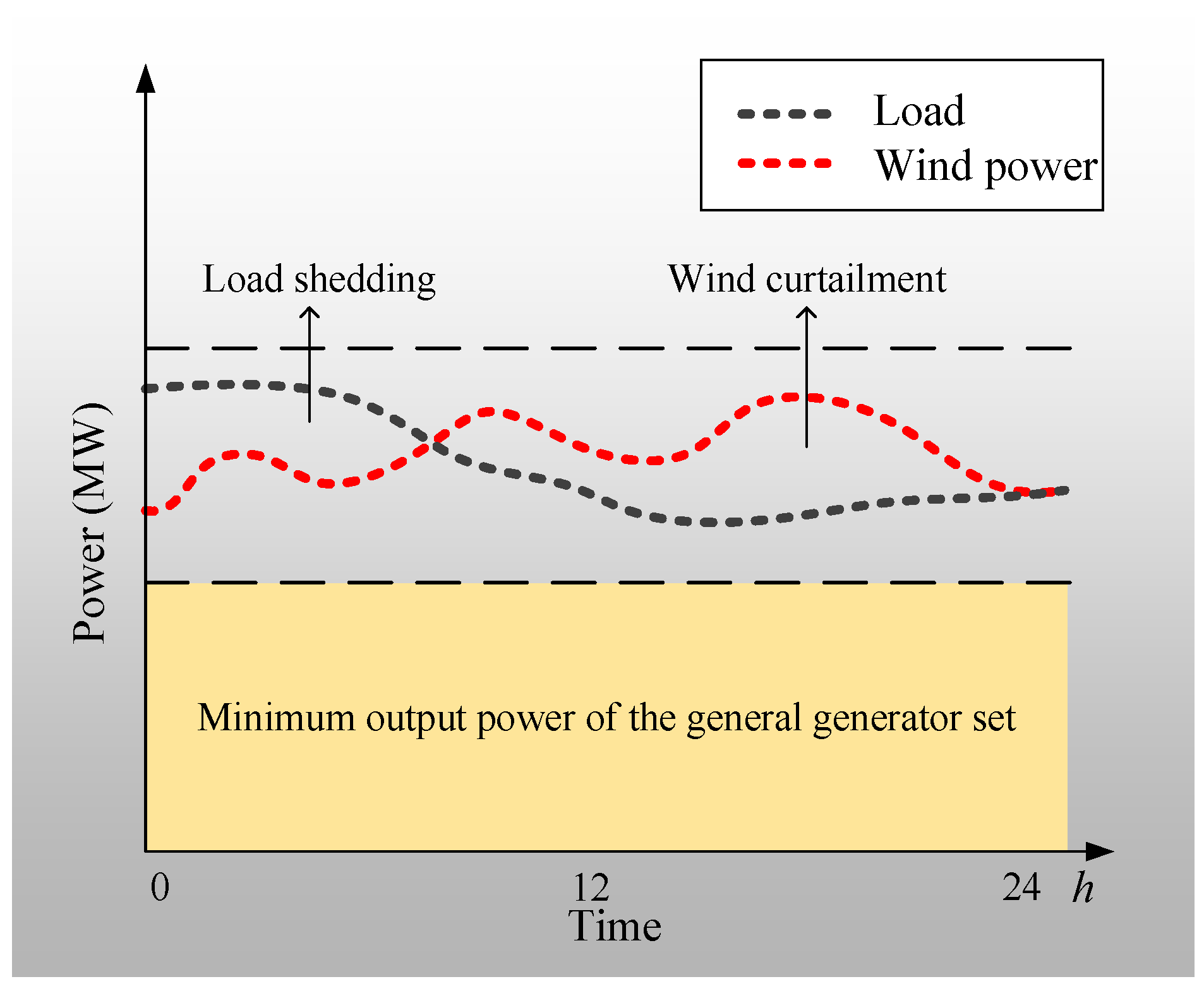
The transmission network is a real-time balance system, but high-penetration wind power and variable load will affect this balance. Hence, when the wind farm output power is greater than the maximum absorbable power of the system or the adjacent lines of the wind farm do not have enough capacity to transmit the power flow, the excess wind power needs to be curtailed to ensure the balance. On the contrary, when the system load power exceeds the sum of the power of wind farm and the general generator set or the adjacent lines of load node are blocked, the excess load will be shed. Figure 1 is the schematic diagram of wind curtailment and load shedding.

We set priority wind power output conditions to ensure the maximum wind power consumption. Therefore, the wind curtailment is determined by the load and the minimum output of general generator set. The wind curtailment of each hour $p_{wind,h}^{curt}$ is calculated by

$$p_{wind,h}^{curt}={\displaystyle {\sum }_{N_{wind}}^{}{P}_h^{wind}}+{\displaystyle {\sum }_{N_G}^{}{P}_h^{\min }-{\displaystyle {\sum }_{N_{Load}}^{}{P}_h^{load}}}$$

(19)

where N_wind is the total number of wind farms; $P_h^{wind}$ is the sum of the output of wind farm at h-th hour; $P_h^{\min }$ is the sum of the minimum output of general generator set at h-th hour; $P_h^{load}$ is the sum of the input of load at h-th hour.

The total wind curtailment of each scenario $P_{wind}^{curt}$ is

$$P_{wind}^{curt}={\displaystyle {\sum }_{h=1}^{24}{p}_{wind,h}^{curt}}.$$

(20)

The load shedding of each hour $P_{load,h}^{shed}$ is

$$p_{load,h}^{shed}={\displaystyle {\sum }_{N_{wind}}^{}{P}_h^{wind}}+{\displaystyle {\sum }_{N_G}^{}{P}_h^{\max }-{\displaystyle {\sum }_{N_{Load}}^{}{P}_h^{load}}},$$

(21)

where $P_{j,h}^{\max }$ is the maximum output of general generator set j at h-th hour.

The total load shedding of each scenario $P_{load}^{shed}$ is

$$P_{load}^{shed}={\displaystyle {\sum }_{h=1}^{24}{p}_{load,h}^{shed}}.$$

(22)

The wind curtailment and load shedding can evaluate the operation economy of system structure under uncertain scenarios. However, the high-penetration wind power and variable load may cause the line with excessive power flow to be cut off, which will lead large-scale power flow transfer and even cause a cascading failure. We propose to apply the improved electrical betweenness to measure system power flow balance in uncertain scenarios, and use it to evaluate the system stability.

The stability evaluation of the transmission network based on the electrical betweenness integrates the power flow characteristics into the topology analysis. This method uses electrical betweenness to indicate the transmission power of each line in multiple scenarios, and the large electrical betweenness means that the line is more important in the power flow transmission. When it is forced to be cut off, the system will be severely affected. Therefore, it is necessary to balance the power flow transmission by constructing new lines to improve the system’s ability to withstand uncertainties of wind power and variable load.

The electrical betweenness is based on two assumptions:

Assumption (a): The line power flow is a linear additive model, and the line transmission capacity is shared by each generator set and load.

Assumption (b): The power flow transmission occurs in any line between the generator set and the load.

The calculation of electrical betweenness first requires the system to be divided into a combination of a single generator set and a single load. Then, the combination is required to transmit unit power with the complete line structure. The active power flow P_l,unit and reactive power flow Q_l,unit of line l under transmitting unit power are

$$P_{l,unit}=V_{j,unit}^2(G_{j0}+G_{jk})-V_{j,unit}{V}_{k,unit}(B_{jk}\sin {\theta }_{jk,unit}+G_{jk}\cos {\theta }_{jk,unit}),$$

(23)

$$Q_{l,unit}=-V_{j,unit}^2(B_{j0}+B_{jk})+V_{j,unit}{V}_{k.unit}(B_{jk}\cos {\theta }_{jk,unit}-G_{jk}\sin {\theta }_{jk,unit}),$$

(24)

where V_j,unit and V_k,unit are the voltage of node j and node k under transmitting unit power; G_j0 is the conductivity between node j and ground points; B_jk is the susceptance between node j and node k under transmitting unit power.

Second, the coefficient ω of unit power flow is determined by the smaller value of the generator set and load in the selected combination. The unit power coefficient is calculated by

$$\omega =\{\begin{array}{l}\min \{P_{wind},P_{load}^{vari}\}ifthecombinationcontainswindgeneratorandvariableload\\ \min \{P_{wind},P_{load}^{const}\}ifthecombinationcontainswindgeneratorandconstantload\\ \min \{P_g,P_{load}^{vari}\}ifthecombinationcontainsgeneralgeneratorandvariableload\\ \min \{P_g,P_{load}^{const}\}ifthecombinationcontainsgeneralgeneratorandconstantload\end{array},$$

(25)

where $P_{load}^{vair}$ and $P_{load}^{const}$ are the power of variable load and constant load.

Third, all combinations in the system should be traversed, and the electrical betweenness of lines can be obtained from the sum of the unit power flow distribution. The electrical betweenness (EB) is

$$EB={\displaystyle {\sum }_{s\in \mathsf{\Phi }}^{}\omega (P_{l,unit,s}+}{Q}_{l,unit,s}),$$

(26)

where Φ is the combination set; s is a combination of one source and one load.

The (26) can compare the power flow of each line in the system, but it is difficult to intuitively calculate the power flow balance of the system. Therefore, this paper proposes to use the Wasserstein distance to measure the uniformity of electrical betweenness distribution.

The Wasserstein distance measures the similarity of two distributions by calculating the distance between two distributions. In this paper, the Wasserstein distance between the electrical betweenness distribution and the absolute equilibrium power flow EB_balance distribution is used to evaluate the power flow balance of the transmission network. Additionally, the power flow Wasserstein distance Wass(EB) is

$$Wass(EB)=\underset{\gamma ~\prod (EB,E{B}_{balance})}{\inf }{\mathbb{E}}_{(EB,E{B}_{balance})~\gamma }[\Vert EB-E{B}_{balance}\Vert ],$$

(27)

where inf means infimum; Π(EB, EB_balance) represents the set of all possible joint probability distributions of EB_l,h and EB_balance; ‖A‖ is any norm of A.

The lower-level objective function needs to improve the system’s renewable energy consumption capacity while ensuring that the system has a small improved electrical betweenness. Therefore, the lower-level objective function f_lower(·) is

$$f_{lower}(\cdot )=\min {\left[P_{wind}^{curt},P_{load}^{shed},Wass(EB)\right]}^T.$$

(28)

2.2.4. Lower Constrains

The lower-level constraints are similar to the upper-level constraints, and they are

$$P_j^g-P_{wind,j}^{curt}-V_j{\displaystyle {\sum }_{k\in j}(G_{jk}\cos {\theta }_{jk}+B_{jk}\sin {\theta }_{jk})=}{P}_j^{load}-P_{load,j}^{shed},$$

(29)

$$Q_j^g-Q_{wind,j}^{curt}-V_j{\displaystyle {\sum }_{k\in j}(G_{jk}\sin {\theta }_{jk}+B_{jk}\cos {\theta }_{jk})=}{Q}_j^{load}-Q_{load,j}^{shed}-Q_j^c,$$

(30)

$$V_j^{\min ,lower}\le V_j\le V_j^{\max ,lower},$$

(31)

$${\theta }_j^{\min ,lower}\le {\theta }_j\le {\theta }_j^{\max ,lower},$$

(32)

$$P_j^{g,\min }\le P_j^g\le P_j^{g,\max },$$

(33)

$$P_j^{wind,\min }\le P_j^{wind}\le P_j^{wind,\max },$$

(34)

$$Q_j^{g,\min }\le Q_j^g\le Q_j^{g,\max },$$

(35)

$$-F_l^{\max }\le F_l\le F_l^{\max },$$

(36)

$$0\le P_{wind,j}^{curt}\le {\mu }_j^{wind}{P}_j^{wind},$$

(37)

$$0\le P_{load,j}^{shed}\le {\mu }_j^{load}{P}_j^{load}.$$

(38)

The solution of this model is to find a transmission network structure that meets various constraints and maximizes the performance of the objective function. The method based on deep reinforcement learning determines the construction value of each line based on Markov decision to realize the TNEP task. The method based on heuristic learning achieves the optimization goal by iterating the overall transmission network structure, while business optimizer such as CPLEX is based on mathematical planning to solve the task model.

3. Multi-Agent DDQN for Transmission Network Expand Planning

This section proposes multi-agent DDQN based on deep reinforcement learning for the bi-level TNEP model solving. First, the task environment model of TNEP is constructed based on the Markov Chain model. Second, an improved multi-agent DDQN is proposed according to the characteristics of the task model, which realizes the coordinated solution of the upper-level and lower-level models. Finally, we provide the improved multi-agent DDQN training process for the TNEP task.

3.1. Task Environment of Transmission Network Expansion Planning Based Markov Chain Model

The TNEP scheme is determined by the current system requirements and the established network structure. When each line is constructed, the system structure will be transformed into a new state, and the operation state will also be improved. This work can be abstracted into a Markov serialized decision process, and the schematic diagram of Markov Chain model for TNEP task is shown in Figure 2.

The Markov Chain model provides a way to solve the task through sequential decision. The reinforcement learning uses this mechanism to build task environment and agent for task solving. The task environment can provide the agent with the current task state and executable actions. The agent chooses actions according to a certain strategy. The task environment changes the task state according to the selected action, then calculates the reward of the action and transmits it to the agent. Therefore, the task environment ζ_TNEP can be expressed in state space as:

$${\zeta }_{TNEP}=[S,A,R,\gamma ],$$

(39)

where S is set of task state; A is set of executable action; R is set of action reward; γ is discount factor.

In Figure 2, the current system structure is considered as the initial state S_t, and each line construction is considered as an action A_t. The probability of transition from state S_t to state S_t+1 is p(S_t, S_t+1). When a line is constructed to the state change to state S_t, the system operational improvement is considered as a reward R_t. The state value and state-action pair value are defined as v(S_t) and q(S_t, A_t). When state S_t transforms into the state S_N, the cumulative reward is G(S_t).

The Markov decision assumes that the generation of a new state is only related to the current state, and the state transition probability p(S_t, S_t+1) is

$$p\left(S_{t+1}\mid S_t\right)=p\left(S_{t+1}\mid S_1,\dots ,S_t\right).$$

(40)

When the state S_t−1 changes to the state S_t, the reward R_t is

$$R_t=\mathbb{E}\left[R_{t+1}|S_t\right]$$

(41)

where $\mathbb{E}\left[R_{t+1}|S_t\right]$ means the expectation of all action rewards in the state S_t.

The transition from the state S_t to the state S_t+1 is triggered by action A_t. The probability of action A_t is selected under the state S_t is defined as p(A_t|S_t). If the action selection is based on the policy π, the probability of action selection can be written as

$$\pi (A_t|S_t)=p(A_t|S_t),$$

(42)

The state S_t has an influence on all subsequent states, but the farther from S_t, the smaller the influence. The reward obtained by S_t in the subsequent state also has this characteristic. Therefore, the cumulative reward G(S_t) of each path can be defined as

$$G(S_t)={\displaystyle \sum _{k=0}^N{\gamma }^k}{R}_{t+k+1},$$

(43)

where γ is discount factor.

The state value v(S_t) is expressed by the expectation of cumulative reward obtained by each path from S_t based on policy π, and the relationship between G(S_t) and v_π(S_t) is

$$\begin{array}{l}{v}_{\pi }(S_t)={\mathbb{E}}_{\pi }\left[G(S_t)\mid S_t\right]\\ ={\mathbb{E}}_{\pi }\left[{\displaystyle \sum _{k=0}^{\infty }{\gamma }^k}{R}_{t+k+1}\mid S_t\right]\\ ={\mathbb{E}}_{\pi }\left[R_{t+1}+\gamma G(S_{t+1})\mid S_t\right]\\ ={\mathbb{E}}_{\pi }\left[R_{t+1}+\gamma v_{\pi }(S_{t+1})\mid S_t\right]\end{array},$$

(44)

The action value of action A_t under the state S_t based on policy π is defined as q_π(S_t, A_t). Therefore, v(S_t) can be written as the weighted sum of action value. That is

$$v_{\pi }(S_t)={\displaystyle \sum _{A_t\in \psi }\pi (A_t\mid S_t)q_{\pi }(S_t,A_t)},$$

(45)

where Ψ is the action set of state S_t.

The relation between q(A_t|S_t) and v(S_t+1) is

$$q_{\pi }(S_t,A_t)=R_{t+1}+\gamma {\displaystyle \sum _{S_{t+1}\in \Lambda }p\left(S_{t+1}\mid S_t\right)}{v}_{\pi }(S_{t+1}),$$

(46)

where Λ is the state set of state S_t+1.

Substitute (46) into (45), it obtains

$$v_{\pi }(S_t)={\displaystyle \sum _{A_t\in \psi }\pi (A_t\mid S_t)[R_{t+1}+\gamma {\displaystyle \sum _{S_{t+1}\in \Lambda }p\left(S_{t+1}\mid S_t\right)}{v}_{\pi }(S_{t+1})]}.$$

(47)

Both (46) and (47) are Bellman equations, and the value function can be calculated iteratively through the dynamic programming. If the policy π is determined, the transition probability p(S_t+1|S_t) and the action selection probability π(A_t|S_t) are known. Therefore, we only need to optimize the value function to promote the cumulative reward, and the TNEP task can be solved according to the optimal state sequence.

3.2. Multi-Agent DDQN Structure

DDQN is a value-based deep reinforcement learning. Its crucial objective is to construct and train an accurate value function for the value prediction of state-action pairs. The DDQN agent takes the action based on the ε-greedy strategy and value function to change the task state. Meantime, it modifies the value function through the reward of task state changes. The principle diagram of DDQN is shown in Figure 3.

DDQN contains two value functions, Q_eval and Q_target, with the same initial parameters based on the deep neural networks. This paper uses the Tensorflow platform to build the deep neural network, and the parameters of DDQN are shown in

Table 1. Parameters of DDQN in Tensorflow platform.

Parameters	Value
Learning rate	0.01
Discount factor	0.90
ε-greedy	0.90
Maximum number of episodes	200
Number of hidden layers	4
Number of hidden neurons	32, 64, 128, 256
Optimizer	Adam
Activation	Relu

.

Q_eval is used to select the optimal value action. Through the value perdition of the action A_t-state S_t pair, the best action A^max(S_t;ω_eval) is

$$A^{\max }(S_t;{\omega }_{eval})=\arg \underset{A_t}{\max }{Q}_{eval}(S_t,A_t;{\omega }_{eval}),$$

(48)

where D(a;b) denotes the variable D with respective to the variable a and the parameter b; ω_eval is the parameters of deep neural network Q_eval.

Q_target is used to predict the best action value. The best action value Q^max(S_t;ω_target) is

$$Q^{\max }(S_t;{\omega }_{target})=Q_{target}(S_t,A^{\max }(S_t;{\omega }_{eval});{\omega }_{target}),$$

(49)

where ω_target is the parameters of deep neural network Q_traget.

According to (46), the reward q(S_t,A_t) of action A_t-state S_t pair can be obtained as

$$q(S_t,A_t)=R_{t+1}+\gamma Q^{\max }(S_{t+1};{\omega }_{target}).$$

(50)

The value function loss Q_loss of Q_eval is

$$Q_{loss}=q(S_t,A_t)-Q_{eval}(S_t,A_t;{\omega }_{eval}),$$

(51)

after each action is executed, the Q_eval update regulation is

$$Q_{eval}^{t+1}=Q_{eval}^t+\alpha Q_{loss},$$

(52)

where α is learning rate of DDQN; $Q_{eval}^{t+1}$ and $Q_{eval}^t$ are the $Q_{eval}$ state at t-th time and t + 1-th time, and the parameters ω_eval of Q_eval are copied into Q_target periodically. This delayed update mechanism can ensure stable iteration of parameters.

Based on the bi-level model of TNEP, we built a dual of DDQN agent. One set is used to search the economical transmission network. The upper-level model reward R_upper is

$$R_{upper}=V_{base,upper}-f_{upper}{\left[f_1(l),f_2(l),f_3(l)\right]}^T,$$

(53)

where V_base,upper is the reward baseline of upper-level agent.

The other set is used to optimize the wind curtailment, load shedding, and improve electrical betweenness of transmission network. The lower-level model reward R_lower is

$$R_{lower}=V_{base,lower}-f_{lower}{\left[P_{wind}^{curt},P_{load}^{shed},Wass(EB)\right]}^T.$$

(54)

where V_base,lower is the reward baseline of lower-level agent.

In the optimization of the bi-level model, we stipulate that the upper-level agent needs to store the top three economical lines to form a Pareto set. The constitution rule of the upper-level solution set Pareto{A_t,upper} is

$$\mathrm{Pareto}\{A_{t,upper}\}=\{\begin{array}{l}\mathrm{First}\mathrm{three}{A}^{\max }(S_t;{\omega }_{eval,upper})\mathrm{Prob}\ge \epsilon \\ \mathrm{Three}{A}_t\mathrm{obtained}\mathrm{randomly}\mathrm{Prob}<\epsilon \end{array}$$

(55)

where Prob is the random probability of ε-greedy strategy.

The optimization scope of the lower-level DDQN agent should be in (55). The constitution rule of lower-level action A_t,lower is

$$\begin{array}{c}{A}_{t,lower}=\{\begin{array}{ll}{A}^{\max }(S_t;{\omega }_{eval,lower})& \mathrm{Prob}\ge \epsilon \\ \mathrm{One}{A}_{t,upper}\mathrm{obtained}\mathrm{randomly}& \mathrm{Prob}<\epsilon ,\end{array}\\ s.t.:A_{t,lower}\in \mathrm{Pareto}\left\{A_{t,upper}\right\}\end{array}$$

(56)

When each selected action A_t,lower is executed, the Q_eval,upper and Q_eval,lower update based on (56). The multi-agent DDQN flow chart of TNEP task is shown in Figure 4, where Q_eval,lower and Q_eval,upper is used to select the optimal value action of lower-level agent and upper-level agent, respectively; Q_target,lower and Q_target,upper is used to predict the best action value of lower-level agent and upper-level agent, respectively; R_t+1,upper and R_t+1,lower is reward of state S_t+1 of lower-level agent and upper-level agent, respectively.

4. Simulation and Verification

In this section, we apply the multi-agent DDQN to solve the multi-scenarios TNEP tasks of system with high-penetration of RES. The planning scheme and solution process of multi-agent DDQN are compared with those of DQN, particle swarm optimization (PSO) and branch-and-bound (B&B) in the modified IEEE RTS-24 bus system and the modified New England 39-bus system.

4.1. Modified IEEE RTS-24 Bus System with High-Penetration RES

The IEEE RTS-24 bus system is widely used to evaluate the performance of planning algorithms. This model contains 24 generator or load buses. The initial network consists of 38 lines with two rated voltages, the north area is 220 kV and the south area is 110 kV. The load model contains 17 buses with a maximum of 2850 MW. The generation model contains 32 generator sets, and the range of the output is 12–400 MW.

Based on the IEEE RTS-24 bus system, a modified IEEE RTS-24 bus system is constructed, in which the types of some generator sets and loads are changed to make the system have the characteristics of renewable energy and variable load. The changes are listed in

Table 2. Changes of generator set and load in the modified IEEE RTS-24 bus system.

Node	IEEE RTS-24 Bus System	Modified IEEE RTS-24 Bus System	Power (MW)
1, 13, 18, 23	general generator set	wind farm set	192, 591, 400, 660
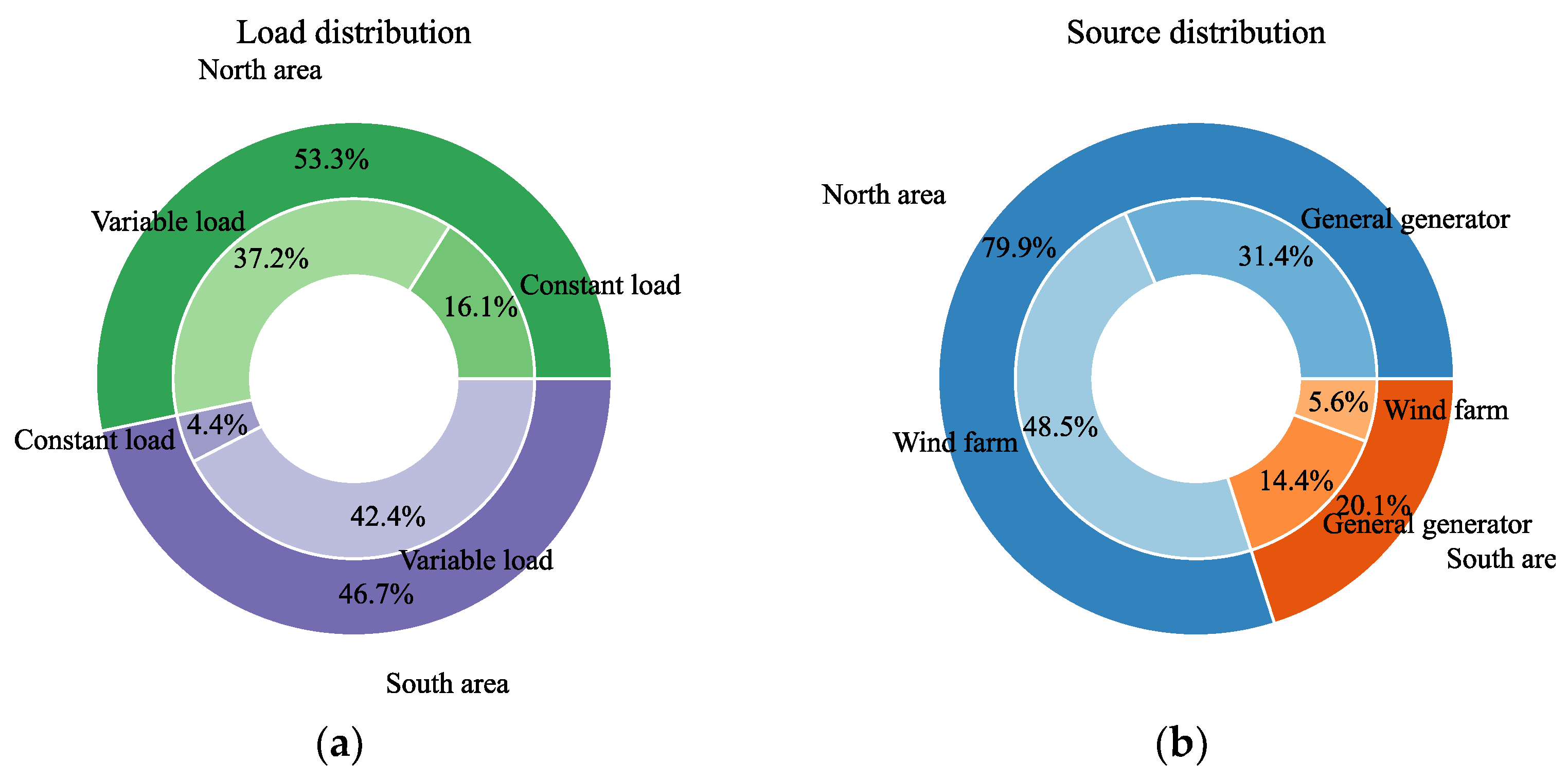
1, 2, 3, 4, 6, 7, 8, 15, 16, 18, 19, 20	constant load	variable load	108, 97, 180, 74,136, 125, 171, 317, 100, 333, 181, 128

, and the distribution of generator set and loads is shown in Figure 5.

It can be seen from Figure 5 that the modified system contains 54.1% renewable energy and 79.6% variable load, which simulates the high-penetration renewable energy and variable load characteristic of RES system.

Then, we use the improved K-Means algorithm to extract the typical scenarios. Its performance is not only related to the setting of the clustering objective function, but also closely related to the K value. We use the improved K-Means algorithm to cluster the variable wind power and load operation data of HRP-38-test-system in reference [31], and the best K value is determined from the curve of SSE based on the elbow method. The results are shown in Figure 6.

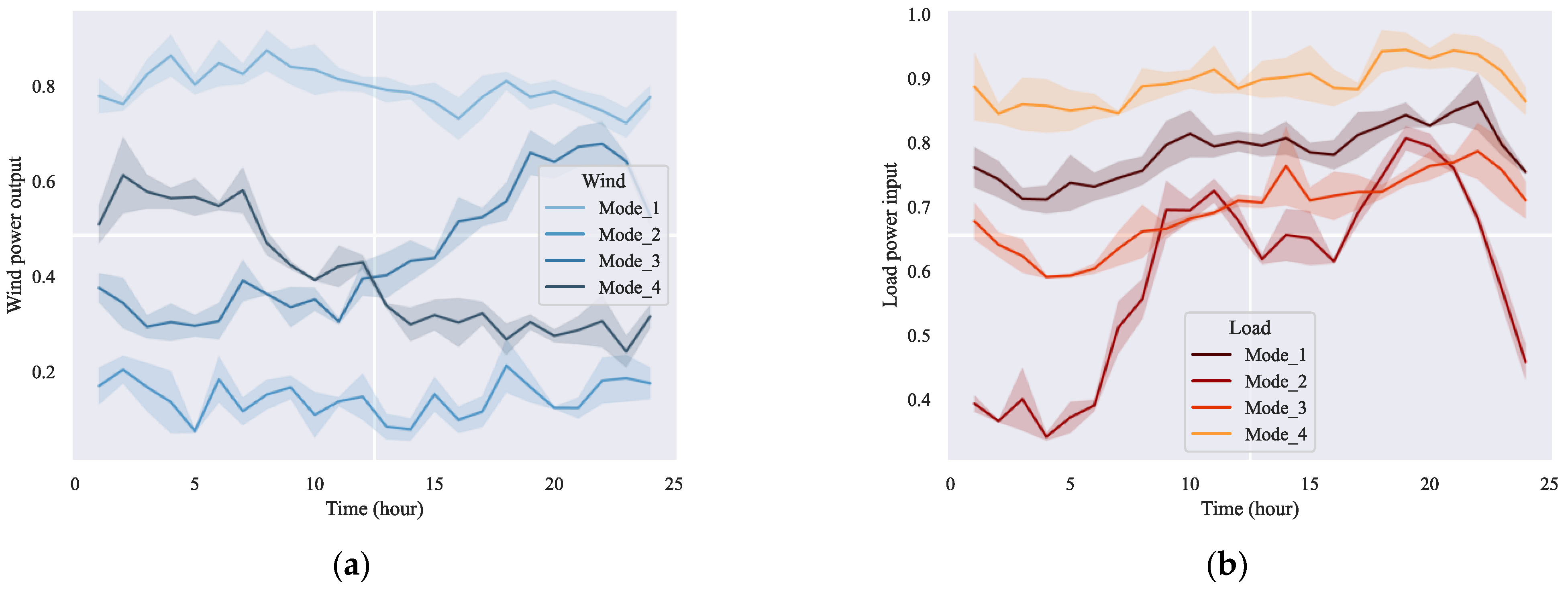
The results show that the SSEs of wind power and variable load decreases faster when K value becomes K = 4. If K continues to increase, the change rate of SSE will decrease, which can be considered as an elbow point. Therefore, this paper adopts K = 4. The clustering results are shown in Figure 7.

Figure 7a shows the four operating modes of wind power. Mode 1 and mode 2 are distinguished by the difference in cumulative energy. Mode 3 and mode 4 have similar cumulative energy, but the fluctuation characteristics are different. Similarly, in Figure 7b, the cumulative energy of load 1, 3, and 4 modes are different, and the fluctuation characteristics of mode 2 are more unique. Therefore, the improved K-Means algorithm realizes the operation data compression of wind power and variable load, which greatly improves the efficiency of TNEP task solving.

The scenario generation rule is to randomly select the wind farm and load status in each hour from the extracted mode as the system status and then generate 384 typical scenarios. Some typical scenarios are listed in

Table 3. Typical scenarios in the modified IEEE RTS-24 bus system.

System Status	Wind Farm Power Output	Variable Load Power Input	Treatment
lack of power	0.072506	0.918429	wind curtailment
excess of power	0.730986	0.336237	load shedding
high-level dynamic balance	0.433848	0.471544	None
Low-level dynamic balance	0.719905	0.736917	None

.

The typical scenarios cover the normal and extreme conditions during the system operation. This data-driven scenario generation method reduces computational complexity and ensures the uncertain characteristic.

4.2. TNEP for Multi-Level Renewable Energy Penetration Scenarios in Modified IEEE RTS-24 Bus System

All the programs are developed using TensorFlow 1.14 and python 3.7. The system configuration is i9-9900K with 3.6 GHz, a memory of 32 GB, and graphics card of 2080Ti. DQN and PSO are used for contrast, and the parameters of multi-agent DDQN and DQN are listed in

Table 4. Parameters of multi-agent DDQN and DQN.

Parameter	Multi-Agent DDQN Value	DQN Value	Unit
maximum learning number	200	200	episode
maximum iteration number of each episode	150	150	step
number of neural network layers	50	50	layer
neural network copy parameter interval	200	None	step

. The TNEP schemes of four methods are shown in

Table 5. TNEP scheme of multi-agent DDQN in modified IEEE RTS-24 bus system.

Lines Number and Sequence	Upper Level (Comprehensive Cost)			Lower Level
	Line Construction Cost (USD (millions))	Network Loss Cost (USD (millions))	Operation and Maintenance Cost (USD (millions))	Improved Electrical Betweenness	Wind Curtailment (MW)	Load Shedding (MW)
None	0.00	4.01	9.04	0.007154	80.11	227.22
11–15	1.51	3.21	8.95	0.005584	64.60	141.88
22–23	2.20	2.96	8.94	0.005155	60.67	105.43
14–15	2.87	2.90	8.96	0.004927	57.74	95.92
20–22	3.55	2.81	8.98	0.004732	60.21	80.62
1–2	3.67	2.81	8.96	0.004751	60.22	80.62
2–7	4.53	2.81	9.03	0.004795	60.44	57.78
13–15	6.95	2.72	9.13	0.004457	44.20	57.61

,

Table 6. TNEP scheme of DQN in modified IEEE RTS-24 bus system.

Lines Number and Sequence	Comprehensive Cost			Improved Electrical Betweenness	Wind Curtailment (MW)	Load Shedding (MW)
	Line Construction Cost (USD (millions))	Network loss Cost (USD (millions))	Operation and Maintenance Cost (USD (millions))
None	0.00	4.01	9.04	0.007154	80.11	227.22
11–15	1.51	3.21	8.95	0.005584	64.60	141.88
13–15	3.93	3.02	9.04	0.005493	51.57	130.62
7–8	4.57	2.92	9.05	0.005676	51.57	92.16
9–12	6.57	2.93	9.15	0.005813	47.80	90.36
16–17	7.65	2.84	9.19	0.005214	47.20	71.06
14–15	8.32	2.81	9.22	0.004994	46.62	62.68
7–9	10.58	2.81	9.33	0.005108	47.03	51.59

,

Table 7. TNEP scheme of PSO in modified IEEE RTS-24 bus system.

Lines	Comprehensive Cost			Improved Electrical Betweenness	Wind Curtailment (MW)	Load Shedding (MW)
	Line Construction Cost (USD (millions))	Network Loss Cost (USD (millions))	Operation and Maintenance Cost(USD (millions))
7–8	7.81	2.39	9.11	0.00518	86.61	75.64
11–15
12–13
13–20
14–15
14–20
22–23

and

Table 8. TNEP scheme of B&B in modified IEEE RTS-24 bus system.

Lines	Comprehensive Cost			Improved Electrical Betweenness	Wind Curtailment (MW)	Load Shedding (MW)
	Line Construction Cost (USD (millions))	Network Loss Cost (USD (millions))	Operation and Maintenance Cost (USD (millions))
1–5	10.41	2.64	9.31	0.005182	68.45	65.09
7–8
8–10
11–15
12–23
17–19
18–19

, and the transmission network structure is in Figure 8.

Table 5, Table 6, Table 7 and Table 8 show that all four methods optimize the stability and economy of the transmission network by constructing lines. The deep reinforcement learning based methods contain line sequence information, but PSO method only optimizes the structure of the complete transmission network structure. Among the four schemes, the scheme obtained by multi-agent DDQN has the lowest construction cost at USD 6.95 M. Due to the scheme obtained by DQN includes the line 9–12, which contains a set of transformers, the construction cost is the highest at USD 10.58 M. In addition, the four schemes all affect the system structure and the distribution of power flow through new lines construction, which decreases the network loss cost. Finally, the objective function of the upper-level model is to minimize the comprehensive cost. The comprehensive costs of four methods are USD 18.8 M, USD 22.72 M and USD 19.31 M, USD 22.36 M, respectively. The scheme obtained by multi-agent DDQN has the lowest comprehensive cost, which proves that the one set DDQN agent built by the upper-level layer is better than DQN agent in the optimization of comprehensive cost indicators.

The improved electrical betweenness measures the system stability by calculating the power flow balance of each line. The scheme obtained by multi-agent DDQN reduces the improved electrical betweenness from 0.007154 to 0.004457, which reduces the probability of cascading failures than other three methods. In addition, system with high-penetration of RES needs to ensure as little wind curtailment and load shedding as possible under uncertain scenarios. Both multi-agent DDQN and DQN improve the power support capability through building a tighter transmission network structure. However, the scheme obtained by PSO is over-searching for a structure with better comprehensive cost performance, and it ignores the optimization of the improved electrical betweenness, wind curtailment and load shedding. This is because the heuristic learning-based method is easy to fall into the local optima problem in TNEP task solving processing. TNEP is a complex non-convex non-deterministic polynomial (NP) problem. The scheme obtained by B&B still has a certain gap with the other schemes obtained by three methods. The methods based on deep reinforcement learning well coordinates the optimization of the lower-level model indicators, which avoids the impact of the local optima problem to a certain extent, and confirms the superiority of this type of methods in this task.

Although the sum of the wind curtailment and the load shedding are nearly equal for scheme obtained by DQN and multi-agent DDQN, the improved electrical betweenness of multi-agent DDQN is significantly better. The dual DDQN agent structure improves the optimization capability of each layer, and thus forming a better solution method for TNEP task.

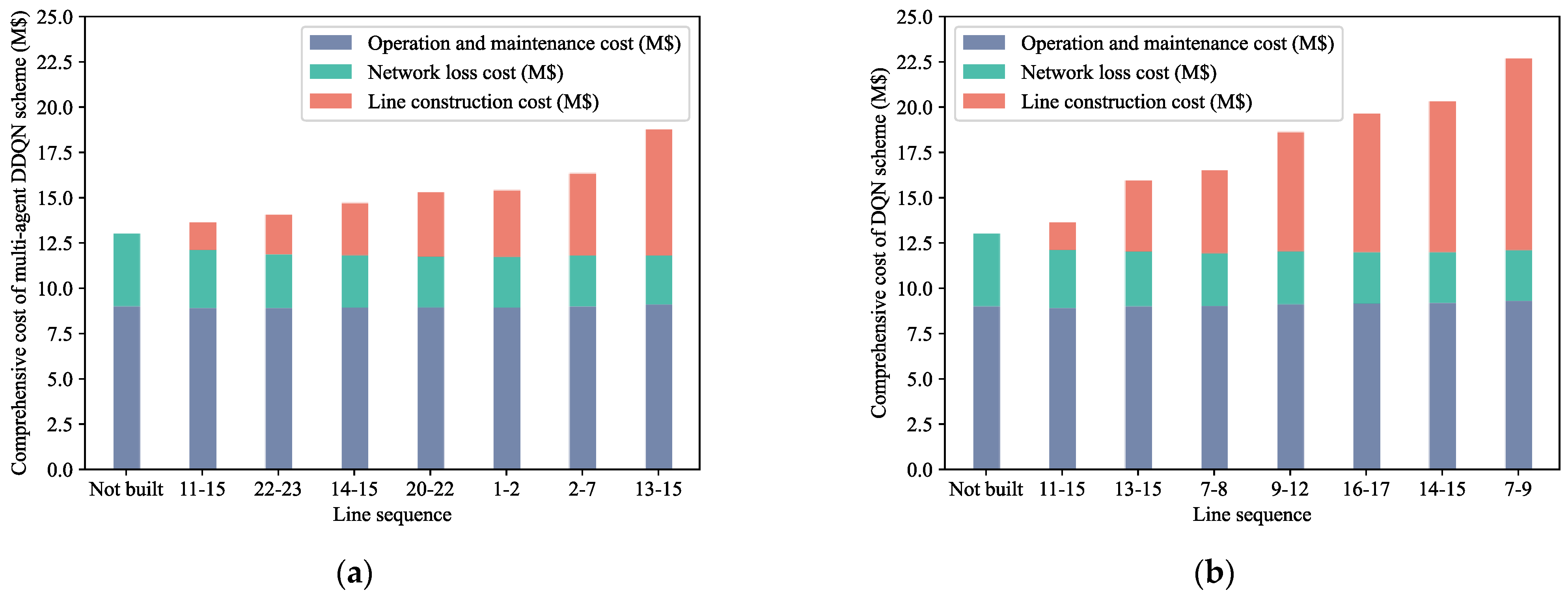
Figure 9 shows the comprehensive cost changes of the schemes obtained by multi-agent DDQN and DQN. The construction cost of lines 13–15, 9–12, and 7–9 in the DQN scheme is relatively high, which makes the construction cost rise rapidly. The scheme obtained by multi-agent DDQN chooses lines with lower construction cost, so that the investment in the scheme implementation can be invested more smoothly. Moreover, the sum of network loss cost and operation and maintenance cost of scheme obtained by multi-agent DDQN are decreasing faster, which makes the transition process more economical.

Figure 10 is the distribution of line power flow for the two methods. It shows that the initial power flow is quite uneven, and the power flow of the initial network contains three lines with more than 300 MW and two lines more than 400 MW. The scheme obtained by multi-agent DDQN transfers part of the power flow to underloading lines, which improves the utilization rate of the underloading lines and reduces the probability of the cascading failures caused by the overloading lines. For the lines with power greater than 200 WM in Figure 10b, the multi-agent DDQN controls the line power flow close to 250 MW. The scheme obtained by DQN reduces most of the line power flow to below 250 MW, but it contains two lines that are much larger than 250 MW. For the lines with power lower than 200 MW, multi-agent DDQN optimizes the power flow distribution in the range of 150~200 MW better than DQN method. DQN better increases the power flow of underloading lines, and multi-agent DDQN tends to limit the power flow of overloading lines. The lines with high power flow often determine the stability of the system. Therefore, the scheme obtained by multi-agent DDQN has higher system stability.

Figure 11 shows the changes in wind curtailment and load shedding during the construction of the two schemes.

The initial network structure sheds a mass of load under uncertain scenarios. When the output of wind farms is reduced, the regional power balance ability is weakened, and the power support from power generators and wind farms in the other regions of the system is needed to supplement the regional power shortage. However, when the congestion occurs in transmission lines connected to the power shortage area, the power support in the system is difficult to achieve, which forces load shedding. Therefore, it is necessary to build new lines to eliminate the occurrence of congestion. The two schemes obtained by multi-agent DDQN and DQN both reduce the load shedding to the same level through new lines construction, and multi-agent DDQN is decreasing slightly faster than the scheme obtained by DQN. The wind curtailment of the multi-agent is lower than the scheme obtained by DQN, more wind power will be curtailed during the construction process.

Multi-agent DDQN not only controls the sum of wind curtailment and load shedding as DQN, but also obtains a scheme with high power flow balance. This demonstrates that one set DDQN agent built by lower-level model has better performance than DQN agent for lower-level optimization. Therefore, the dual DDQN agent structure realizes the hierarchical prediction value of line. One set is used to search the lines with high economy, and the other set is to search the lines that can improve the renewable energy consumption capacity and stability of the system. This structure improves the accuracy of the line value prediction and contributes to the formation of a better TNEP scheme.

Figure 12 and Figure 13 are the indicators (such as wind abandonment and load shedding) of 7000 network structures constructed by the multi-agent DDQN agent in 200 episodes of training. Before 1000 steps, the distribution of various indicators in poor areas is more concentrated, or only some indicators of the network perform well. This is because the multi-agent DDQN does not have enough data for neural network training now, and there is a large error in its value prediction. Between 1000 and 2500 steps, the indexes of the transmission network gradually improve. The neural network achieves sufficient training, and the prediction error of the line construction value has gradually decreased. After 2500 steps, the indexes are uniformly distributed between the best and the worst. This is because the multi-agent DDQN adopts a ε-greedy strategy, which allows the agent to chooses the line randomly without using the prediction result of the neural network under a certain probability. This training mechanism can prevent local optimal problem and obtain more accurate value function.

Figure 14 shows the sum of value prediction of multi-agent DDQN and DQN. The value prediction represents the estimation of the construction value estimation of different lines by the agent, and the sum of value prediction of the multi-agent DDQN is lower than that of the DQN. This is because the agent of multi-agent DDQN adopts a dual neural network structure, which makes the optimal line A^max independent of the value prediction Q^max of the optimal line. This structure avoids the influence of accidental overestimation to a certain extent and improves the accuracy of line value prediction, which enhances the ability of multi-agent DDQN to solve TNEP task.

4.3. TNEP under Unavoidable Interference in Modified IEEE RTS-24 Bus System

During the implementation of the TNEP scheme, unavoidable interference or unconsidered factors may cause a certain line to be unable to be constructed. When this happens, the heuristic learning-based method requires retraining due to changes in planning conditions. However, the experience obtained from training based on the reinforcement learning method is to judge the construction value of each line, which is not affected by changes in conditions. Thereby, multi-agent DDQN can solve new TNEP tasks without redundant training. We change the fourth line of the scheme obtained by multi-agent DDQN from 20–22 to line 5–6 to simulate the TNEP task scenario under unavoidable interference. Similarly, the fourth line of the scheme obtained by DQN is changed from 9–12 to line 13–14. The schemes obtained by multi-agent DDQN and DQN are shown in

Table 9. TNEP scheme of multi-agent DDQN in modified IEEE RTS-24 bus system under unavoidable interference.

Lines Number and Sequence	Upper Level (Comprehensive Cost)			Lower Level
	Line Construction Cost (USD (millions))	Network Loss Cost (USD (millions))	Operation and Maintenance Cost (USD (millions))	Improved Electrical Betweenness	Wind Curtailment (MW)	Load Shedding (MW)
None	0.00	4.01	9.04	0.007154	80.11	227.22
11–15	1.51	3.21	8.95	0.005584	64.60	141.88
22–23	2.20	2.96	8.94	0.005155	60.67	105.43
14–15	2.87	2.90	8.96	0.004927	57.74	95.92
5–6	4.41	2.89	9.04	0.005171	57.75	95.94
19–21	5.07	2.83	9.06	0.004801	59.60	83.84
5–7	6.44	2.80	9.12	0.004852	59.60	64.69
13–15	8.86	2.72	9.23	0.004659	44.07	61.32

and

Table 10. TNEP scheme of DQN in modified IEEE RTS-24 bus system under unavoidable interference.

Lines Number and Sequence	Comprehensive Cost			Improved Electrical Betweenness	Wind Curtailment (MW)	Load Shedding (MW)
	Line Construction Cost (USD (millions))	Network Loss Cost (USD (millions))	Operation and Maintenance Cost (USD (millions))
None	0.00	4.01	9.04	0.007154	80.11	227.22
11–15	1.51	3.21	8.95	0.005584	64.60	141.88
13–15	3.93	3.02	9.04	0.005493	51.57	130.62
7–8	4.57	2.92	9.05	0.005676	51.57	92.16
13–14	6.33	2.94	9.14	0.005762	43.63	86.68
18–21	7.41	2.94	9.20	0.006050	43.62	88.76
20–21	8.21	2.88	9.23	0.005555	58.51	58.13
15–19	9.14	2.85	9.27	0.005194	56.34	57.72

.

After the interference, the improved electrical betweenness of the scheme obtained by multi-agent DDQN immediately deteriorates, and the wind curtailment and load shedding are hardly improved. This shows that the line 5–6 causes the system power flow balance to be destroyed, and the scheme is greatly affected by the interference. On the contrary, although the improved electrical betweenness of the scheme obtained by DQN slightly deteriorates after the interference, the line 13–14 reduces the wind curtailment and load shedding. The continued construction of multi-agent DDQN after unfavorable interference is more positive. The multi-agent DDQN agent reuses training experience to judge the performance of the current transmission network structure and the construction value of each line. Then, three high-value lines are selected to form the new scheme. Although the new scheme obtained by multi-agent DDQN increases the comprehensive cost under unfavorable interference, it still shows great performance in the improved electrical betweenness, wind curtailment and load shedding. The comprehensive cost of scheme obtained by new DQN is USD 0.45 M, which is higher than that of the new scheme obtained by multi-agent DDQN. In addition, the improved electrical betweenness of the new scheme obtained by DQN is also larger than that of the new scheme obtained by multi-agent DDQN, which means the new scheme obtained by DQN has lower reliability of the system. Even the excellent control of wind curtailment and load shedding in the scheme obtained by original DQN is weakened. Finally, both methods can complete planning tasks by reusing the training experience under the unavoidable interference, but the value prediction of multi-agent DDQN is more accurate, which makes the multi-agent DDQN better to solve such TNEP tasks.

4.4. TNEP in Modified New England 39-Bus System

This article extends the application scenario to a more complex modified New England 39-bus system to further evaluate the performance of the proposed methods. Consistent with the changes in the modified IEEE 24-bus system, we increase the load to 1.1 times, the capacity of conventional generator sets to 1.2 times, and the capacity of wind farms to 1.4 times. The node settings of wind farm and variable load are shown in

Table 11. Changes of generator set and load in modified New England 39-bus system.

Node	New England 39-Bus System	Modified New England 39-Bus System	Power (MW)
30, 32, 33, 34, 38	general generator set	wind farm set	1040, 725, 652, 508, 865
3, 4, 8, 16, 20, 24, 27, 29	static load	variable load	322, 500, 522, 329, 680, 308.6, 281, 283.5

, the schemes of the four methods are shown in

Table 12. TNEP scheme of multi-agent DDQN in modified New England 39-bus system.

Lines Number and Sequence	Upper Level (Comprehensive Cost)			Lower Level
	Line Construction Cost (USD (millions))	Network Loss Cost (USD (millions))	Operation and Maintenance Cost (USD (millions))	Improved Electrical Betweenness	Wind Curtailment (MW)	Load Shedding (MW)
None	0.00	3.51	14.32	0.007352	350.40	49.49
2–30	2.00	3.53	14.42	0.007649	210.03	49.83
16–19	2.60	3.38	14.44	0.007336	114.82	49.83
2–3	2.90	3.37	14.46	0.007014	74.69	35.88
3–4	3.26	3.34	14.47	0.006559	74.01	35.88
1–2	3.99	3.32	14.51	0.006512	69.48	35.91
10–32	5.99	3.31	14.61	0.006721	39.56	35.88
3–18	6.35	3.28	14.62	0.006197	39.74	35.88

,

Table 13. TNEP scheme of DQN in modified New England 39-bus system.

Lines Number and Sequence	Comprehensive Cost			Improved Electrical Betweenness	Wind Curtailment (MW)	Load Shedding (MW)
	Line Construction Cost (USD (millions))	Network Loss Cost (USD (millions))	Operation and Maintenance Cost (USD (millions))
None	0.00	3.51	14.32	0.007352	350.40	49.49
16–19	0.60	3.36	14.34	0.007078	252.02	48.23
1–2	1.33	3.33	14.38	0.007083	250.54	47.16
16–17	1.65	3.31	14.39	0.006563	250.54	47.22
2–30	3.65	3.34	14.49	0.006824	69.47	45.99
25–26	4.28	3.31	14.52	0.006550	69.40	39.97
16–24	4.92	3.30	14.55	0.006667	69.40	39.97
2–3	5.22	3.31	14.57	0.006276	69.47	35.91

,

Table 14. TNEP scheme of PSO in modified New England 39-bus system.

Lines	Comprehensive Cost			Improved Electrical Betweenness	Wind Curtailment (MW)	Load Shedding (MW)
	Line Construction Cost (USD (millions))	Network Loss Cost (USD (millions))	Operation and Maintenance Cost (USD (millions))
1–39	7.16	3.15	14.66	0.006087	74.54	35.89
2–3
2–30
3–4
16–19
17–18
25–37
26–27

and

Table 15. TNEP scheme of B&B in modified New England 39-bus system.

Lines	Comprehensive Cost			Improved Electrical Betweenness	Wind Curtailment (MW)	Load Shedding (MW)
	Line Construction Cost (USD (millions))	Network Loss Cost (USD (millions))	Operation and Maintenance Cost (USD (millions))
2–3, 2–25, 2–30, 3–18, 9–39, 10–11, 16–19	6.76	3.29	14.57	0.006327	75.40	35.88

, and the network structure is shown in Figure 15.

The generator sets of the modified New England 39-bus system are settled at the edge of the system, but the load nodes are evenly distributed. Under the uncertain scenarios, the initial network structure cannot deliver wind power to the system due to the line blockage, and the system curtails a large amount of wind power. Therefore, the three methods all need to optimize the wind farm adjacent line structure to improve the power transmission capacity under uncertain conditions. The scheme obtained by multi-agent DDQN focuses on optimizing the network structure near node 30 connecting the largest capacity wind farm by adding six new lines (2–30, 1–2, 2–3, 3–4, 3–18, 17–18). In addition, the construction of line 10–32 also raises the upper limit of the transmission capacity of the node 32 wind farm. Although the schemes obtained by DQN and the PSO optimize the node 30 adjacent line structure, their ability to select key lines is still insufficient. The scheme obtained by DQN only optimizes the lines within the distance between two lines near node 30, but it does not further optimize the structure with longer distances. The PSO and CPLEX optimize the node 30 network structure is similar to that of multi-agent DDQN, except that the more influential 1–2 line is ignored. In addition, neither of PSO and DQN optimizes the line structure near other wind farms, which leads to the poor performance in reducing wind curtailment. Although the scheme obtained by B&B optimizes the line structure near the 32-node, it did not choose the 10–32 line that more directly impacts the power transmission of the wind farm. The scheme obtained by multi-agent DDQN has the best improved electrical betweenness and better economy, which proves the advantages of multi-agent DDQN in scheme optimization and multi-objective coordination in complex TNEP tasks.

5. Conclusions

This paper proposes a multi-agent DDQN for the TNEP task considering the uncertainties of wind power and load. In order to extract typical uncertain scenarios for TNEP tasks from system operating data, we improve the K-Means algorithm with the cumulation and the change rate of operation data as the clustering objective function. It improves computational efficiency while retaining the uncertainty of the system. Based on the typical uncertain scenarios, we construct a Bi-level multi-objective TNEP model considering the system renewable energy consumption capacity, economy, stability. Then, we transform the bi-level model into a TNEP reinforcement learning environment based on the Markov Chain model, which can support the interactive way to solve the TNEP task.

Based on the bi-level model structure, the proposed method constructs a dual DDQN agents, which realizes separation of the upper-level and the lower-level objective function optimization. The comparison of the proposed method with other four methods in multi-scenario TNEP tasks shows that the multi-agent DDQN is the most high-performance and flexible method. In addition, it trains by interacting with the reinforcement learning environment, which makes the training process more interpretable and observable than the heuristic-learning based methods. This paper only considers the uncertainties of wind power and load. In future work, we can build a TNEP model that contains more factors such as electric vehicle to expand the application scenarios of this method. Simultaneously, it is necessary to increase the computational efficiency by improving the multi-agent DDQN structure.