
Coupled Basin and Hydro-Mechanical Modeling of Gas Chimney Formation: The SW Barents Sea
by
 , , ,
, , ,
Georgy A. Peshkov
1,* ,
,
Lyudmila A. Khakimova
1,2,3,*,
Elena V. Grishko
1,
Magnus Wangen
4 and
Viktoria M. Yarushina
3,4 1
Center for Petroleum Science and Engineering, Skolkovo Institute of Science and Technology, Territory of Innovation Center “Skolkovo”, Bolshoy Boulevard 30, Bld. 1, 121205 Moscow, Russia
2
Institute of Earth Sciences, University of Lausanne, 1015 Lausanne, Switzerland
3
Faculty of Mechanics and Mathematics, Lomonosov Moscow State University, 119991 Moscow, Russia
4
Institute for Energy Technology, Instituttveien 18, 2007 Kjeller, Norway
*
Authors to whom correspondence should be addressed.
Energies 2021, 14(19), 6345; https://doi.org/10.3390/en14196345
Submission received: 9 August 2021
/
Revised: 31 August 2021
/
Accepted: 29 September 2021
/
Published: 4 October 2021
(This article belongs to the Special Issue Advances in Simulation of Fluid Flow Dynamics in Porous and Fractured Media)
Abstract
:Gas chimneys are one of the most intriguing manifestations of the focused fluid flows in sedimentary basins. To predict natural and human-induced fluid leakage, it is essential to understand the mechanism of how fluid flow localizes into conductive chimneys and the chimney dynamics. This work predicts conditions and parameters for chimney formation in two fields in the SW Barents Sea, the Tornerose field and the Snøhvit field in the Hammerfest Basin. The work is based on two types of models, basin modeling and hydro-mechanical modeling of chimney formation. Multi-layer basin models were used to produce the initial conditions for the hydro-mechanical modeling of the relatively fast chimneys propagation process. Using hydro-mechanical models, we determined the thermal, structural, and petrophysical features of the gas chimney formation for the Tornerose field and the Snøhvit field. Our hydro-mechanical model treats the propagation of chimneys through lithological boundaries with strong contrasts. The model reproduces chimneys identified by seismic imaging without pre-defining their locations or geometry. The chimney locations were determined by the steepness of the interface between the reservoir and the caprock, the reservoir thickness, and the compaction length of the strata. We demonstrate that chimneys are highly-permeable leakage pathways. The width and propagation speed of a single chimney strongly depends on the viscosity and permeability of the rock. For the chimneys of the Snøhvit field, the predicted time of formation is about 13 to 40 years for an about 2 km high chimney.
1. Introduction
Fluid flow tends to be localized in space and time at all length scales within the Earth: from the deep mantle to the shallow subsurface [1,2,3,4]. Focused fluid flows have shaped the planet during its 4.5 billion years history [4,5]. Their variety on Earth is enormous: they often have similar geometry but different origins caused by various geological processes and mechanisms. The understanding of focused fluid flow is a significant challenge because of the non-linear nature of the problem. Today, seismic gas chimneys are among the most common manifestations of the focused fluid flows in sedimentary basins worldwide [6,7,8]. Understanding gas chimney formation and evolution are essential for oil and gas exploration and secure long-term storage of CO2 [9,10,11].
Gas chimneys are vertical fluid escape pathways through sealing rock and overburden rock strata. They are observed in sedimentary basins worldwide [7]. Their morphology is non-unique in terms of scales, seismic signatures, and shapes [12,13]. Interpretations of deteriorated seismic signals provide their present-day location, while circular seafloor craters (pockmarks) indicate the locations in the present and past [8,14]. There are two fundamental mechanisms for the formation of a gas chimney. One is hydraulic fracturing driven by overpressure when fluid pressure exceeds the lithostatic. However, this mechanism would be limited to the upper 1 km of the overburdened rocks since the pressure does not allow for boiling pore fluids [15]. Another mechanism is related to ascending porosity wave propagation through poro-visco-elastoplastic media [16]. That is influenced by rock viscosity, porosity, permeability, and initial subsurface architecture.
Most current research on gas chimneys discusses geological processes leading to chimney formation, e.g., [1,4,17,18,19]. However, only a very few theoretical works with modeling on the reservoir and basin scales are presented. The numerical modeling of the gas leakage and chimney forming mechanisms is very challenging. Tasianas et al. [20] modeled the gas leakage along pre-existing conducting geological structures on the reservoir scale. They considered the flow along three types of structures preliminary set up in the model: faults, fracture network penetrating the reservoir’s caprock, and high permeable fluid conduits. However, they did not consider the processes leading to the formation of these structures. Ostanin et al. [21] considered the basin-scale mechanism of gas leakage by faults sealed during glacial loading and conductive during ice retreat. Duran et al. [22] used the basin modeling approach to estimate the volume of leaked gases from the reservoir to the seafloor. They assumed that flow pathways were formed by a capillary failure of the seal when the upward-directed buoyancy pressure, generated by the lower density of hydrocarbons (HC), plus any excess overpressure in the reservoir exceeds the capillary resistance pressure of the seal. Iyer et al. [15] considered a vent complex for gas leakage. Vent complexes are associated with large igneous provinces globally and are similar to gas chimneys. The vents are considered conduits for fluid and gas phases generated within the contact aureole of the associated magmatic intrusion. Iyer et al. [15] used a simplified ad-hoc modeling approach, assuming that rock permeability increases with increasing pressure and returns to the initial value as fluid pressure drops using the same function.
Few models [16,23,24] attempted to explain chimney formation using the porosity wave mechanism. The porosity wave can transfer fluid through geological layers with low permeability in localized areas with high porosity. The character of this process is spontaneous and self-propagating. Mckenzie [25] initially suggested this type of model to explain the migration of melt in partially molten rocks. Afterward [26], the same model was used for the understanding of sedimentary compaction. Yarushina and Podladchikov [16] created a simple model for porous fluid flow in a deformable matrix. The model can capture the range of rheological responses within Earth’s lithosphere. This model can predict the behavior of fluid-rock systems during sedimentary compaction at a wide range of temperatures and time scales. The model was limited by hydrostatic compaction and decompaction. Later [23], the effects of shear stresses on (de)compaction processes were considered. Based on this model, Rass et al. [24] presented a 3D simulation of the spontaneous development of high-permeability pathways through two geological layers from a fluid-enriched source region. These regions reproduce natural seismic pipes or chimneys. However, these models are based on synthetic datasets and do not consider geological processes on a basin-scale preceding the chimney formation.
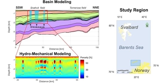
This work addresses the formation of chimney-like focused fluid flow structures in the South-Western (SW) Barents Sea by considering coupled basin- and reservoir-scale modeling. We focused on the Snøhvit and Tornerose fields of the Hammerfest Basin in the SW Barents Sea. The objects’ choice is related to two factors: (1) a good understanding of basin and petroleum systems evolution and (2) the presence of gas chimneys traced from the main reservoir of Stø Formation in the Snøhvit field. Hence, the causal relationships of reasons, duration, and location of gas chimneys are determined [20]. In addition, this object is of great interest to CO2 sequestration. The basin modeling approach provides the chimney location’s thermal, petrophysical, and structural characteristics with seismic data analysis. The followed reservoir-scale hydro-mechanical modeling of gas leakage associated with the porous rock deformations uses outputs from the basin model as an initial setup for simulations.
2. Geological Settings and Petroleum Systems
The geological setting of the epicontinental SW Barents Sea is well studied and described in works, e.g., [26,27,28,29,30], and briefly summarised here, noting the main geological events. SW Barents Sea has experienced a relatively deep basin burial history. The basin accounts for several tectonic episodes of lithosphere extension accompanied by subsidence and basin formation from Devonian to Paleocene-Eocene time [26]. The basin tectonic history begins with the Caledonian Orogeny covering the territory from Greenland to the Norwegian shelf [31]. Extensional episodes from Devonian to Early Cenozoic time with accompanied subsidence formed the segregated SW Barents Sea basins with block-faulted structures presented by highs and troughs [26,32]. Compressional events formed the fault complexes along the boundaries of major structural elements [33]. The Cenozoic period is introduced by uplifts and erosions in the basins and on structural highs, while at the shelf edge, thick progradation structures were deposited [34]. The deep erosion phase began in the Oligocene due to tectonic uplift after the Norwegian-Greenland Sea opening [35]. The rapid decrease of a global temperature in the northern hemisphere occurred at ~2.5 Ma and was accompanied by a regional glaciation [36]. The Pliocene to Pleistocene uplift and erosion associated with the isostatic response of cycle loading of ice-cap determined the late-stage evolution of the SW Barents Sea [34]. The Hammerfest Basin is one of the SW Barents Sea primary oil and gas regions. The basin is enclosed to the south by the Troms–Finnmark Fault Complex, to the west by the Ringvassøy–Loppa Fault Complex, while to the north and east by the Loppa High and the Bjarmeland Platform, respectively (Figure 1). The Hammerfest basin initially was structurally continuous with the Loppa High [35,37]. The Carboniferous extension caused the tilting of the Loppa High and Hammerfest basin to the Early Permian. The isolated sea deposition environment with anoxic episodes formed the Kobbe formation (Fm) as a possible source rock.
During the Late Triassic, the formed accommodation space during subsidence was infilling by sediments. The Late Triassic siliciclastic Snadd Fm is considered a possible source rock. Tectonic subsidence, faulting reactivations, eustatic sea-level changes, and sediments’ deposition controlled the evolution of the margin from the Late Triassic to the Middle Jurassic. Simultaneously, sea-level changes formed the foreshore environment to offshore and estuarine sub-environments strongly influenced by wave processes and tidal effects [39]. The deposition formed the Tubåen Fm and Stø Fm as the main reservoir of the Snøhvit and Tornerose fields. During Middle Jurassic to Late Jurassic, global sea-level rise formed the marine environment for shale sedimentation, mainly the primary source rock Hekkingen Fm [29,35,40]. Transgression sequence in the central part of the Hammerfest Basin during the Middle Paleocene initiated the marine sedimentation. Progradational sedimentation bodies sourced from the platform areas to NNE filled the basin during the Late Paleocene [22].
The Jurassic formations Stø and Tubåen are the primary reservoirs in the Hammerfest Basin according to the petroleum system analysis of Duran et al. [22,40]. The Snøhvit field reservoir is located on the west side of the transect, and the Tornerose discovery is on the east side (see yellow ovals in Figure 2b). The reservoir of Stø Fm in the Snøhvit area consists of natural gas with an oil leg, while Tornerose discovery accumulates pure gas [22,40].
Several gas chimneys traced from the primary reservoir of Stø Fm in the Snøhvit field were observed by different researchers [4,21,22,37] (Figure 2b). Mohammedyasin et al. [37] applied high-quality pre-stack time-migrated (PSTM) 3D seismic data interpretations (Figure 1b) to analyze the gas leakage pathways. Geometrically, the chimneys are determined as tubular-shaped (Chimney 1), cone-shaped (Chimney 2), and Christmas tree-structured (Chimney 3) (Figure 2b). Based on the acoustic masking, the lateral extension of the chimneys varies from ~1 to ~10 km with decreasing depth. Chimney 1 and Chimney 2 decrease laterally downward, while Chimney 3 has a Christmas tree geometry.
Ostanin et al. [21] and Duran et al. [22] consider the Pliocene–Pleistocene glaciation cycles a primary reason for hydrocarbon loss from Stø Fm reservoir. Nevertheless, Ostanin et al. [21] consider the basin fault system a pathway for gas and fluids leakage during ice unloading. In contrast, Duran et al. [22] consider mainly the seal capillary failure during the peak of ice loading. In both works, gas leakage events are associated with several deglaciation periods from 0.02 to 0.01 Ma.
3. Data and Methods
We consider both basin-scale geological processes that preceded the chimney formation and porous fluid flow coupled with deformation processes associated with relatively short and local chimney formation episodes. To capture these processes at different time and length scales, we combine two approaches: basin modeling and coupled hydro-mechanical modeling at the reservoir scale. First, basin modeling allows reproducing the burial history of the basin. It produces the properties of the basin, such as porosity, effective thermal properties, permeability, paleotemperatures, and organic matter maturity rank. Second, we perform coupled hydro-mechanical modeling at the target reservoir-sized domain based on basin modeling results which allows reproducing spontaneous development of gas chimneys. The basin modeling provides the geological setting and the initial conditions for the chimney formation, which is handled within the second simulation step and used as the initial setup for the reservoir-scale hydro-mechanical model.
Chimneys that form due to non-linear hydro-mechanical coupling occur over less than 1 Ma, and its spatial resolution varies from 1 m to 1 km. The non-linear hydro-mechanical coupled model generates fluid escape chimney-like structures cutting through the sedimentary units. The porosity and permeability evolve in time and space within the reservoir-sized domain. However, there is no feedback of these changes back to the basin modeling simulator. Therefore, the impact of the chimneys on the paleo-fluid pressure is not considered.
3.1. Basin Modelling
3.1.1. Burial Histories
Basin modeling aims at reproducing the burial history, subsidence rate, erosion period and rate, sedimentation rate, and thermal history of a sedimentary basin [41]. The modeling considers present-day stratigraphy, including the sedimentary units’ geometry, deposition time, and lithology. The first step in a basin simulation is a calibration of the burial history. It is done by estimating the net thicknesses of (porosity-free) rock in each formation. These net thicknesses remain constant throughout the burial history. The net thicknesses are used in a forward simulation of the burial history, which includes the computation of the porosity of the sedimentary units at each time step. There are two approaches to calibrating the net (porosity-free) thicknesses in the burial history. The so-called “back stripping” method works backward in time by stripping off layer by layer and decompacting the remaining layers. See details in [42]. The decompaction is done using porosity as a function of burial depth. The other approach of estimating the formation thicknesses is to run forward simulations as an iterative process. The net thicknesses are updated at the end of the burial history by comparing them with the present-day thicknesses. The second approach is more general than the first and allows for porosity functions that depend on depth and time, temperature, and pressure [43]. The backstripping approach is decoupled from the simulation of paleo-temperature and paleo-pressure. It is, therefore, decoupled from the forward simulation [44,45,46,47]. In this study, we use the Athy [48] porosity function of depth
where is the porosity at the depth , is surface porosity, B is the compaction length (see Table 1). Each lithology has its surface porosity and compaction length.
In the previous work [49], particularly for the same case study, we compared the present-day state of the basin models derived by both approaches. We used the BMT software [50] to reconstruct the basin history by the backstripping method, while we use the simulator TecMod 2019.1 to reconstruct the basin with iterative forward simulations. Works [44,47] give a detailed description of BMT and TecMod simulators, respectively. Both approaches produced similar results from the point of view of thermal regime and organic matter maturity. Thus, in the present work, we use only the results of the forward modeling approach.
3.1.2. Thermal Histories
Here we briefly review the temperature equation used in basin modeling. A more detailed presentation of heat flow in sedimentary basins can be found in the books of Hantschel and Kauerauf [41], Wangen [43], and Allen and Allen [51].
The temperature equation for transient heat conduction and radiogenic heat production is
where is the bulk density, Cp is the bulk specific heat capacity, k is the bulk thermal conductivity, T is the temperature, z is the vertical coordinate, t is the time, and Q is the radiogenic heat production. The temperature equation is for simplicity written in one dimension for the vertical direction. Notice that the temperature equation does not have a heat convection term. Heat convection may often be ignored in basin simulations, but not always [52].
The bulk thermal conductivity keff is obtained as the geometric mean
of the rock matrix thermal conductivity and fluid heat conductivity [53,54].
The Sekiguchi [55] temperature correction has been applied to rock matrix thermal conductivities. The volumetric bulk heat capacity is obtained by as the arithmetic mean of the volumetric heat capacities of the rock matrix and the fluid [41]
where and are rock matrix and water densities, respectively, and and are rock matrix and water-specific heat capacities, respectively. Both of them include temperature corrections by Waples and Waples [56] and Somerton [57].
A two-dimensional basin has four boundaries. The vertical boundaries are considered isolated, which implies that they have zero heat flux. The surface temperature is assumed known as a function of time. The basin base can either have a given temperature thermal gradient or heat flow as a function of time. The thermal state of the base of the basin is the result of simulations of the entire lithosphere when the basin is fully integrated. If there are no data for the temperature or heat flow at the basin base, the lithosphere can be included in the basin simulation. The lithosphere can be included as a passive domain or as a dynamic domain that undergoes stretching. Lithospheric stretching produces thermal transients that may affect the basin over time spans of several tens of million years [43].
The basin’s thermal model must be calibrated to the data obtained from wells of present-day temperatures and thermal maturity parameters, e.g., vitrinite reflectance [41].
3.2. Hydro-Mechanical Modeling at the Reservoir Scale
Porosity waves were proposed as a mechanism generating focused fluid flow in sedimentary basins [16,23,24,58,59]. They result from the coupling of porous fluid flow and viscous matrix deformations and decompaction weakening [60]. Rock rheology influences the shape of the porosity waves, which can take the form of elongated drops or chimneys [58,60,61].
We use the coupled hydro-mechanical equations to model the spontaneous formation and propagation of high-porosity and permeability channels at the reservoir scale [16]. These equations describe the filtration of incompressible pore fluid coupled with the deformation of the viscous solid matrix.
Mass balances for the rock and pore fluid can be written as
The momentum balances for the solid and fluid phases has a form
where are solid and fluid densities, is the total porosity-averaged density, is the porosity, are the components of solid and fluid velocities, are the total and fluid pressures, are the components of the stress deviator, is the component of the gravity acceleration vector, is the Carman-Kozeny relation (the non-linear porosity-dependent permeability), —the pore fluid viscosity, is the Darcy flux vector.
Within this work, we consider viscous rheology, which is described by the following relation
where is the solid shear viscosity.
The viscous (de)compaction is described by the constitutive equation [16]
where is the solid bulk viscosity, which is porosity dependent and reduced by decompaction weakening factor in the case of overpressure. Equation (10) is the closure relation for the governing system of Equations (5)–(10), which is used for the reservoir modeling of chimneys’ spontaneous formation and evolution.
Rock response is visco-elasto-plastic [62]. Elastic deformation gives an immediate response, while viscous deformation develops on a longer time scale. The relative importance of viscous and elastic terms is controlled by Deborah number introduced in [63]. In our case, the estimation of Deborah is based on the typical values of elastic moduli presented in [62]. Previous model studies show that viscous deformation is essential for forming focused fluid flow [60,64,65,66]. For Deborah numbers from the range of elastic properties don’t significantly impact the formation of focused fluid flow [63,67]. Therefore, in our simulations, we keep only viscous deformation which gives the first-order effect.
The process of focused fluid flow affected by viscous deformation is characterized by compaction length
and viscous compaction time
where is the dynamic permeability, is the fluid viscosity, is the effective bulk viscosity, is the difference in densities of the rock and fluid, is the gravity constant.
4. Modeling Results
4.1. Basin Modeling
4.1.1. Dataset from the Hammerfest Basin
A transect from the Hammerfest basin was simulated with TecMod2D 2019.1. The burial history begins with the deposition of the Ørret Fm in Permian, a little more than 250 Ma ago. Sixteen layers represent the stratigraphy from the Late Permian to the present-day seabed (Figure 2). In the model, each layer has its lithology (Table A1). There are no lateral changes of the lithologies, except for the main reservoir in the Stø Fm, which changes laterally from sandstone (Stø Fm 01) to siltstone (Stø Fm 02) at the lateral position of 28 km (Figure 3a). The lithology description of each layer and corresponding petrophysical properties are presented in Appendix A based on work [22]. The Oligocene-Miocene erosional event occurs between 29–15 Ma [22]. The eroded thicknesses range from 140 to 840 m, and the thicknesses are increasing from southwest to northeast. This erosional scenario corresponds to the average appraisal of eroded thickness. We follow this scenario since it produces the average porosity for the reservoir among scenarios with a deviation range not higher than ±2%. The glacial activity during Pliocene-Pleistocene is ignored in the model, even though the glaciation and/or deglaciation impact the pore fluid pressure. Nevertheless, we do not consider this event as a critical trigger for the chimney formation.
The lithosphere was included in the simulations. The initial thickness of the upper crust, lower crust, and mantle are 20 km, 20 km, and 100 km, respectively. The modeling of rifting processes assumes differential thinning of the crust and the mantle. The Hammerfest basin has experienced four rift phases, according to Reemst et al. [34] and Skogseid et al. [68]. The model includes only three of them (Triassic, Jurassic-Cretaceous, Palaeocene-Early Eocene) since the first rift phase (Devonian-Carboniferous) was earlier the first horizon in the model.
The boundary condition at the lithosphere base is a constant temperature of 1300 °C [69,70]. The basin surface is either subaerial or underwater. The surface is bounded by the temperature that varies between 10 to 25 °C through the Paleozoic-Pleistocene period [71]. Temperature does not go above 3 °C in the interglacial Pleistocene periods [72,73]. Therefore, the surface temperature is taken to be 6 °C at present [74].
The study uses TecMod’s automatically reconstructed paleo-water depth [47].
4.1.2. Calibration
The stratigraphy was automatically calibrated by the simulator [47,75]. Less than 10 forward simulations were needed to match the present-day layers’ thicknesses. The relative difference between the simulated and observed formation thicknesses is less than 1%.
The calculated thermal parameters were calibrated against temperature and vitrinite reflectance data from a series of wells. These wells are 7120/6-1, 7121/4-1, 7121/4-2, 7121/5-1, which are close to position 50 km on the profile, and to wells 7120/7-1, 7120/7-2, 7120/7-3, 7120/8-1; 7120/8-2 close to lateral position 29 km [23] (and links therein) (Figure 1b). The vitrinite reflectance was computed using the EASY-Ro model [76].
4.1.3. Results
According to Mohammedyasin et al. [37], three chimneys are observed only in the Snøhvit area tracing from the Stø Fm to the seafloor. For a chimney to leak out the gas in a reservoir, the gas must overcome the high capillary threshold of the seal. The Fuglen Fm is the primary seal of the reservoir in the Stø Fm [22,40]. The seal thickness of the Stø Fm in the Tornerose area is up to ten times higher than in the Snøhvit area (Figure 3a). The low thickness of the seal in the Snøhvit area makes it vulnerable for the Oligocene-Miocene erosional event and cycles of glaciation during the Pliocene-Pleistocene. The units above the seal are more coarse-grained, less compacted, and less cemented. These lithological units have properties that allow a chimney to form and to conduct the gas upward.
We observe the higher reservoir thickness with higher porosity of up to 18–22% in the area of Snøhvit field than in Tornerose field (Figure 3b). Thus we assume that this reservoir characteristic is the most optimal for chimney formation [49].
At Palaeocene, the maximum temperatures for the surface of Kobbe Fm source rock in the Snøhvit area reach ~185–190 °C, while the Tornerose area reaches not higher than 140–150 °C (Figure 4). A temperature higher than 170 °C indicates that the secondary cracking of oil to gas [77] was realized. Such thermal conditions contribute to the formation of thermogenic gas, increasing overpressure in the overlying rocks. Other source rocks, Snadd Fm and Hekkingen Fm, experienced lower peak temperatures than 170 °C for both fields (Figure 4).
Underneath the Snøhvit area, at the present day, the surface of the Kobbe Fm is located in the wet gas window, the surface of Snadd Fm—in the main oil window, while the Hekkingen Fm—predominantly in early oil window by Tissot and Welte [78] (see Figure 5). Underneath the Tornerose area, the temperatures and vitrinite reflectance values are significantly lower than in the Snøhvit area. Only the surface of Kobbe Fm is located in the main oil window. The oil in the Snøhvit reservoir area seems to have migrated from the Upper Jurassic Hekkingen Fm, which is in accordance with the petroleum system analysis of Duran et al. [22,40]. The high maturity of the Triassic Snadd Fm and Kobbe Fm source rocks is responsible for the high volumes of gas migrating to the Jurassic reservoirs.
4.2. Hydro-Mechanical Modeling at the Reservoir Scale
4.2.1. Initial Reservoir Model Based on Dataset from the Hammerfest Basin
To provide chimney formation simulation on the reservoir scale, we consider the target reservoir-sized domain (~ km) of the basin model presented in Figure 6. This domain has a simplified structure of layers lumped by their lithology characteristics and porosity distribution given in the basin model. Table 2 summarises the ranges of porosity values corresponding to a specific layer of the target domain.
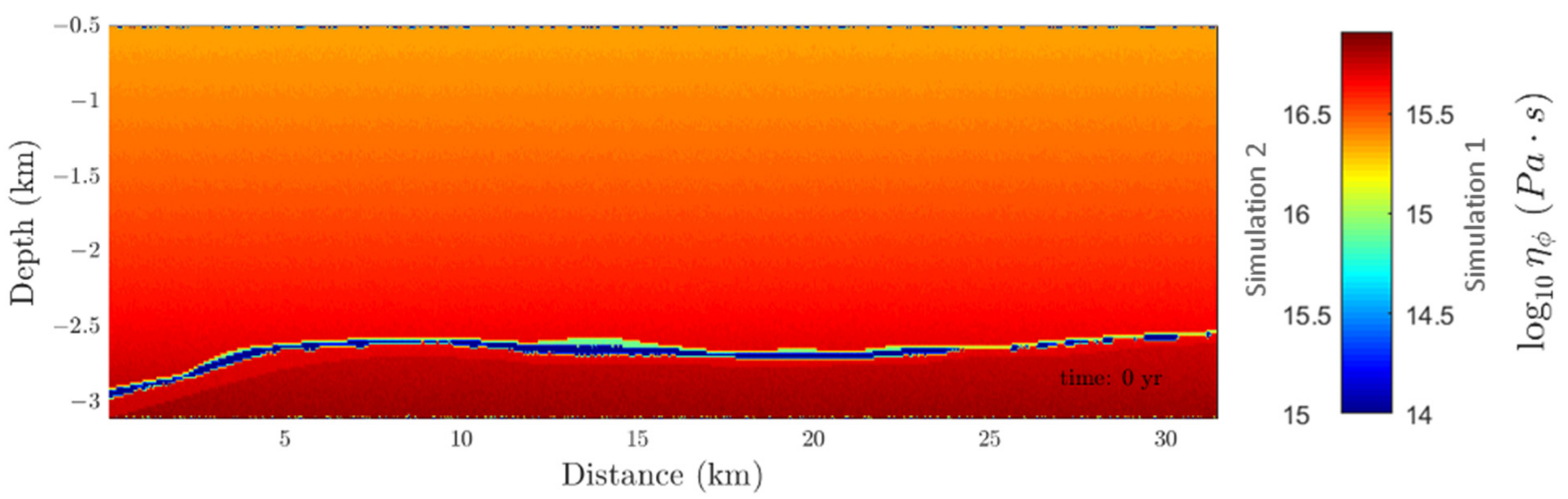
We use coupled hydro-mechanical model (5)–(10) presented in Section 3.2 to simulate the formation and propagation of high-porosity chimneys across the target region. The model does not take into account the fault system since, according to seismic investigations [37], the chimneys’ distribution zones are located far from faults. Thus, the faults are not the plumbing system for these three chimneys. Numerical implementation includes discretizing (5)–(10) using a finite-volume technique on a regular Cartesian grid in 2D in MATLAB. The computational domain has a resolution of grid points. The mechanical part of (5)–(10) was solved using free-slip (no shear stress) boundary conditions on all sides of the computational domain. For the fluid flow part, we utilized no flux boundary conditions on all vertical sides of the computational domain, and fixed flux values at the bottom and top boundaries. Initial conditions for the numerical simulation are presented in Figure 7 and Figure 8, namely initial porosity, dynamic permeability, and bulk viscosity distribution. The initial porosity of the model (Figure 7a) corresponds to the values from the basin model. Figure 7b shows the initial dynamic permeability, , which varies in the range of depending on the specific layer. The pore-fluid density is assumed to be . The solid is twice less buoyant than the pore-fluid. The fluid shear viscosity equals [24].
Within this work, we performed a sensitivity analysis of the numerical model to the initial values of effective bulk viscosity, which is not very well constrained by the laboratory data [24]. For these purposes, we performed two simulations with different ranges of initial effective bulk viscosities. The considered values are taken from [24,62,80]. The initial effective bulk viscosity, , is presented in Figure 8 and has values in the range of in the first simulation and in the second one.
The process of chimneys formation and propagation affected by viscous deformation is characterized by compaction length and viscous compaction time given by Equations (11) and (12).
The fluid density is assumed to be twice less than the solid one. Since the target reservoir domain has a multi-layered structure, we have different values of compaction length (3–300 m and 10–1000 m in the first and the second simulation, respectively) depending on a layer considered in the system (Figure 9). Note, the characteristic time and length are used to non-dimensionalize the problem.
4.2.2. Chimney Modeling Results
Figure 10 and Figure 11 show the evolution of high-porosity chimneys produced in numerical simulations for two cases of lower and higher effective bulk viscosities of reservoir layers. We observe fluid flow episodes which form chimney-like patterns reflecting the multi-layered structure of the considered domain. Chimneys need about 13 years to reach the surface in case of lower effective bulk viscosity values (). For the other case, developed high porosity channels take the larger time to get to the surface, namely around 40 years. The existence of a low-permeable weak shale layer significantly delays the formation of focused fluid flow pathways, which is observed during both simulations. According to the simulation results, channels need about 8 and 25 years to rise through the shale layer in case of lower and higher effective bulk viscosities of reservoir layers, respectively. The resulting locations of high-porosity chimneys are represented in Figure 11a,b. Developed chimneys resulting from the simulation with higher effective bulk viscosities of reservoir layers are characterized by larger width, corresponding to the larger compaction length values. The numerical simulation results are compliant with the identified seismic chimney zones in the target reservoir-size domain shown in Figure 11c. In the middle of the considered domain, seismic data shows a wide chimney, while numerical results predict the formation of a large number of separate smaller channels. These smaller channels might not be resolved individually in seismic and might be seen as one large chimney instead. Results show that the formation of high-permeable channels is associated with topological gradient and the location of initial porosity anomalies. Besides, there is a tendency to accumulate porosity anomalies near lithological boundaries associated with the seal rock (Figure 10) with a following on porosity wave penetration through it.
5. Discussion
Based on basin modeling results, we can infer that chimney formation requires a combination of several factors. Firstly, the source rocks should be mature by being in the wet gas window. Hydrocarbon generation from overmature source rocks creates overpressure in the reservoir. Secondly, the reservoir rock should have a large capacity for long-term gas preservation under high pressure, which is the source for chimney formation. Thirdly, the seal should have low thicknesses (less than hundreds of meters), and additionally, it must lose its integrity by deformation from the tectonic movements and diagenesis.
At this step, we characterized the conditions of chimney zones formation from basin and petroleum system modeling points of view. Comparing the Tornerous and Snøhvit fields, it was found that the latter is in the most favorable conditions for the chimney formation. Next, for chimney modeling on the reservoir scale, we take from the basin model the area of the Snøhvit field. Thus, reservoir, seal rock and overburden rock geometry, and distribution of porosity are extracted.
The results of our basin modeling are different from the results presented in Duran et al. [22] and Ostanin et al. [21]. The previous works used a basal heat flow trend as the lower boundary condition to a basin bottom during the thermal history reconstruction (see Section 3.1.2). Thus, the temperature Equation (2) is solved only for a basin domain. The heat flow accounts only for a response from the lithosphere deformation but ignores the blanketing effect [81,82], when the deposition of “cold” sediments may lead to depressed vertical thermal gradients if the sedimentation rate is “large”. The work [46] demonstrated that using the lower thermal boundary condition that ignores the blanketing effect and thermal effect from erosion of the sediments leads to the estimation of HC generation up to 86%. Thus, the estimates of transformation ratio (TR), a mass of generated HC, and timing of expulsion, migration, and preservation for the analyzed source rocks Kobbe Fm, Snadd Fm, and Hekkingen Fm can contain similar errors despite satisfying well data calibration in works of Duran et al. [22] and Ostanin et al. [21]. Therefore, the gas leakage volumes can be overestimated too. The evidence of temperature overestimation over time without accounting for the blanketing effect is presented in Figure 12. In the Snøhvit area, the surface of Kobbe Fm by Ostanin et al. [21] has higher temperature values up to 45 °C, although the values are matched at present-day. The overestimation of temperature results in a higher maturity rank. For instance, the present-day value of Snadd Fm in the Snøhvit area is estimated as ~1.05 Ro% [21], while the estimates of the present work are close to 0.8 Ro%. Therefore, to obtain the consistent thermal history of the basin, it is required to account for lithosphere deformation during basin evolution and to set the lower boundary condition at the lithosphere bottom to consider the blanketing effect. Otherwise, the calibration of the thermal model against well data is only localized fitting.
Another point of the criticism is connected with the suggested mechanisms of chimney formation. The earliest petroleum system models [22,83] proposed the mechanism of gas leakage as capillary failure in the absence of faults. The capillary failure happened due to the pressure increasing during several glaciation cycles. However, Ostanin et al. [21] proven that the overpressure does not reach the fracture gradients for the Fuglen Fm and Hekkingen Fm seal rocks. Furthermore, in the present work, we showed that the source rocks formations’ temperature history was overestimated, leading to overestimating overpressure, inducing the capillary failure.
Thus, the basin model of Ostanin et al. [21] considers the primary mechanism of gas chimneys formation due to the fault system. Faults were assumed to be partially sealing or conductive during glacial unloading due to significant deviatoric stresses and isostatic compensation and closed during glaciation due to subsidence. According to the modeling, the peak pressure coincides with peak glaciations. In a previous study by Ostanin et al. [84], the fault system of the same dataset was studied in great detail. Also, several amplitude anomalies associated with the gas clouds have been identified based on the high RMS acoustic impedance contrast. Authors claim that all the anomalies are crosscut and follow the strike of faults or are bounded by the 1st order faults [84]. Based on the study of results in [79], we suppose that the conclusion that gas chimney shape follows the faults’ strike or bounded by the 1st order faults is far-fetched. Some of the anomalies are identified out of any 1st and 2nd order faults. The azimuth of the gas cloud does not coincide with the azimuth of the 1st order faults, also as the fault inclination has no similar geometry to the gas cloud. In addition, the mechanism of four and more cycles of fault drainage activation and deactivation by uniform ice load is justified but only assumed. Also, the fault properties depend on several factors, including the degree of disaggregation, dissolution, cementation and mineral precipitation, cataclasis, and stress state [85,86,87].
In the work of Mohammedyasin et al. [37], the plumbing system is interpreted from seismic not only by soft reflections but also by acoustic masking. The soft reflections are interpreted into two groups of anomalies: structurally unconformable to the background reflectors and structurally conformable (aligned in the same direction as the background reflectors). The last is stratigraphically controlled and has no spatial relationship with the deep-seated faults. The acoustic masking analysis helped to delineate three chimneys, as shown in Figure 2b. The author of the work emphasized that the geometry of chimneys signifies fluid leakage at different times for Christmas-Tree (Chimney 3) and regular and consistent leakage for cone-shaped (Chimney 1 & 2). Because of the large lateral extension of each chimney from 1 to 10 km, the authors suggest that more hydrocarbons were leaked from the reservoir through the chimneys. However, in conclusion, the authors give a primary role of pathways for gas leakage to deep-seated faults because most of the trapped gas is on the hanging wall along the section of the major faults [37]. This justification has a weak point since the trapped gas indicates that escaping the gas is difficult. In contrast, the evidence of a chimney with a uniformly distributed not trapped gas confirms the evidence of regular and consistent leakage of fluid in the study area.
In the present work, we consider that the chimney takes the primary role of the gas escape from the reservoir with the porosity wave mechanism. In contrast, the leakage by fault drainage, capillary failure, and molecular diffusion takes the secondary role. We agree with the previous studies that the glacial loading creates a triggering overpressure to leak the fluids. Therefore, it launches the propagation of porosity waves. There are examples where the chimneys are observed, but the glacial loading lacks [88,89,90,91,92,93,94]. Other overpressure-forming mechanisms such as the organic matter maturation, avalanche shelf sedimentation [93], or salt tectonic [94], could play a role in these regions.
To simulate localized highly-permeable channels in the SW Barents Sea, we use the reservoir-sized coupled hydro-mechanical model with the initial conditions coming from the basin modeling. The model suggests porosity waves in porous media with decompaction weakening as a primary mechanism for the spontaneous formation of chimneys. Simulation results reproduce natural observations of chimney-like focused fluid flow structures seen in seismic data. Besides, reservoir simulations show the presence of smaller channels that are possibly below the seismic resolution. The location of modeled chimneys is controlled by stratigraphic layers’ topology, thickness, and compaction length. Our results show that the chimney’s width and propagation speed strongly depend on the compaction length, , given by Equation (11), and viscous compaction time, , given by Equation (12), which are functions of material parameters of layers such as effective bulk and shear viscosity and permeability. Reducing permeability or increasing porous fluid shear viscosity by one order of magnitude will reduce the compaction length by factor 3 and increase the time of chimney formation by the same factor. At the same, reducing solid bulk viscosity by one order of magnitude will reduce both the compaction length and the time of chimney formation by the same factor 3. The essential feature of our work is a coupling of the reservoir- and basin-scale modeling and prediction of spontaneous formation of chimney structures without artificially pre-defined flow pathways.
6. Conclusions
In this paper, we combine basin and reservoir scale models to understand the nature of seismic chimney as focused fluid flow.
A reservoir-scale hydro-mechanical model, being based on geological settings produced by basin modeling, allows for the predicting of chimney-like focused fluid structures in the reservoir cap rock. The model involves fluid flow coupled with viscous deformation of permeable rock, with a decompaction weakening effect.
The results of basin modeling suggest that the lack of chimneys above the Tornerose field is due to insufficient pressure from immature source rocks, in addition to poor temperature conditions for secondary cracking.
The basin model of the Snøhvit field provides a geological environment favorable for chimney formation. The huge gas clouds above the Snøhvit formation are considered gas-filled chimneys, which are produced by porosity wave propagation. It is concluded that chimney formation is the primary reason for the assumed gas leakage from the reservoir.
The steepness of the reservoir-caprock interface, the thickness of layers, location of initial porosity anomalies are found to be a reason for the high-permeable chimneys and their localization. The chimney formation takes about 13 to 40 years to reach the seafloor, depending on the considered values of bulk viscosity of the layers, while the primary resistance occurs in the seal rocks.
Author Contributions
Conceptualization, V.M.Y., L.A.K. and G.A.P.; methodology, V.M.Y., L.A.K. and G.A.P.; software, G.A.P., L.A.K. and M.W.; validation, M.W., L.A.K. and G.A.P.; formal analysis, V.M.Y., L.A.K., E.V.G. and G.A.P.; investigation, E.V.G., L.A.K. and V.M.Y.; resources, G.A.P.; data curation, V.M.Y.; writing—original draft preparation, G.A.P., L.A.K. and E.V.G.; writing—review and editing, M.W. and V.M.Y.; visualization, G.A.P. and L.A.K.; supervision, V.M.Y.; project administration, V.M.Y.; funding acquisition, V.M.Y. All authors have read and agreed to the published version of the manuscript.
Funding
This work is jointly supported by the Russian Fund for Basic Research (Grant no. 18-55-20008) and the Research Council of Norway (Grant no. 280953). L.A.K. and V.M.Y. gratefully acknowledge support from the Ministry of Science and Higher Education of the Russian Federation (project No. 075-15-2019-1890).
Institutional Review Board Statement
Not applicable.
Informed Consent Statement
Not applicable.
Data Availability Statement
The data are available upon request with reasonable purpose via an email to the correspondence author.
Acknowledgments
We would like to express our special appreciation and thanks to late A.V. Myasnikov at Lomonosov Moscow State University and Skoltech, who contributed to the paper at the early stages with insight and helpful discussions. Special thanks are also for J. Pedersen and E. Lundin for data sharing and helpful suggestions. We thank S. Stanchits at Skoltech for project administration and helpful discussions. L.A.K. thanks Yury Podladchikov, Yury Alkhimenkov and Ivan Utkin for inspiring discussions and comments related to the study. We are very grateful to Geomodeling Solutions for providing the TecMod 2019 software.
Conflicts of Interest
The authors declare no conflict of interest.
Appendix A

Table A1.
Material properties and lithological characteristics of modeled stratigraphic units (based on [22]).
Table A1.
Material properties and lithological characteristics of modeled stratigraphic units (based on [22]).
| Physical Properties A | ||||||||
|---|---|---|---|---|---|---|---|---|
| Layer | Color B | Lithology | ϕ0 | B | ρ | k | Cρ | Q |
| (km) | (kg/m3) | (W/m/K) | (J/kg/K) | (μW/m3) | ||||
| Nordland Gp | Siltstone (organic lean) | 0.55 | 1.96 | 2720 | 2.05 | 921 | 1 | |
| Torsk Fm | Shale (organic lean, typical) | 0.70 | 1.20 | 2700 | 1.70 | 879 | 2 | |
| Kveite-Kviting fms. | Siltstone (organic lean) | 0.55 | 1.96 | 2720 | 2.05 | 921 | 1 | |
| Kolmule Fm | Shale (organic lean, silty) | 0.67 | 1.20 | 2700 | 1.77 | 879 | 2 | |
| Kolje Fm | Shale (typical) | 0.70 | 1.20 | 2700 | 1.64 | 879 | 2 | |
| Knurr Fm | Shale (typical) | 0.70 | 1.20 | 2700 | 1.64 | 879 | 2 | |
| Hekkingen Fm | Shale (organic rich, 8% TOC C) | 0.70 | 1.20 | 2500 | 1.20 | 879 | 3 | |
| Fuglen Fm | Shale (organic lean, siliceous, typical) | 0.70 | 1.20 | 2710 | 1.90 | 879 | 1 | |
| Stø Fm 01 | Sandstone (typical) | 0.41 | 3.23 | 2720 | 3.95 | 837 | 1 | |
| Stø Fm 02 | Siltstone (organic lean) | 0.55 | 1.96 | 2720 | 2.05 | 921 | 1 | |
| Nordmela Fm | Siltstone (organic lean) | 0.55 | 1.96 | 2720 | 2.05 | 921 | 1 | |
| Tubåen Fm | Sandstone (clay poor) | 0.42 | 3.33 | 2700 | 5.95 | 837 | 0 | |
| Fruholmen Fm | Siltstone (organic rich, 2–3% TOC) | 0.55 | 1.96 | 2700 | 2.00 | 921 | 1 | |
| Snadd Fm | Siltstone (organic rich, 2–3% TOC) | 0.55 | 1.96 | 2700 | 2.00 | 921 | 1 | |
| Kobbe Fm | Siltstone (organic rich, 2–3% TOC) | 0.55 | 1.96 | 2700 | 2.00 | 921 | 1 | |
| Havert-Klappmys fms. | Shale (organic lean, silty) | 0.67 | 2.33 | 2700 | 1.77 | 879 | 2 | |
| Ørret Fm | Siltstone (organic lean) | 0.55 | 2.44 | 2720 | 2.05 | 921 | 1 | |
References
- Berndt, C. Focused fluid flow in passive continental margins. Philos. Trans. Royal Soc. A Math. Phys. Eng. Sci. 2005, 363, 2855–2871. [Google Scholar] [CrossRef]
- Iyer, K.; Rupke, L.; Galerne, C.Y. Modeling fluid flow in sedimentary basins with sill intrusions: Implications for hydrothermal venting and climate change. Geochem. Geophys. Geosyst. 2013, 14, 5244–5262. [Google Scholar] [CrossRef] [Green Version]
- Hurst, A.; Cartwright, J. Sand Injectites: Implications for Hydrocarbon Exploration and Production; American Association of Petroleum Geologists: Tulsa, OK, USA, 2007; Volume 87. [Google Scholar]
- Vadakkepuliyambatta, S.; Bünz, S.; Mienert, J.; Chand, S. Distribution of subsurface fluid-flow systems in the SW Barents Sea. Mar. Petrol. Geol. 2013, 43, 208–221. [Google Scholar] [CrossRef] [Green Version]
- Patterson, C. Age of meteorites and the earth. Geochim. Cosmochim. Acta 1956, 10, 230–237. [Google Scholar] [CrossRef]
- Hovland, M.; Judd, A. Seabed Pockmarks and Seepages. Impact on Geology, Biology and the Marine Environment; Graham & Trotman: Bath, UK, 1988. [Google Scholar]
- Judd, A.G.; Hovland, M. Seabed Fluid Flow: The Impact on Geology, Biology and the Marine Environment; Cambridge University Press: Cambridge, MA, USA, 2007. [Google Scholar]
- Rise, L.; Sættem, J.; Fanavoll, S.; Thorsnes, T.; Ottesen, D.; Bøe, R. Sea-bed pockmarks related to fluid migration from Mesozoic bedrock strata in the Skagerrak offshore Norway. Mar. Petrol. Geol. 1999, 16, 619–631. [Google Scholar] [CrossRef]
- Bachu, S. CO2 storage in geological media: Role, means, status and barriers to deployment. Prog. Energy Combust. Sci. 2008, 34, 254–273. [Google Scholar] [CrossRef]
- Benson, S.; Cole, D.R. CO2 sequestration in deep sedimentary formations. Elements 2008, 4, 325–331. [Google Scholar] [CrossRef]
- Bickle, M. Geological carbon storage. Nat. Geosci. 2009, 2, 815–819. [Google Scholar] [CrossRef]
- Hustoft, S.; Bünz, S.; Mienert, J. Three-dimensional seismic analysis of the morphology and spatial distribution of chimneys beneath the Nyegga pockmark field, offshore mid-Norway. Basin Res. 2010, 22, 465–480. [Google Scholar] [CrossRef]
- Ostanin, I.; Anka, Z.; di Primio, R.; Bernal, A. Hydrocarbon plumbing systems above the Snøhvit gas field: Structural control and implications for thermogenic methane leakage in the Hammerfest Basin, SW Barents Sea. Mar. Petrol. Geol. 2013, 43, 127–146. [Google Scholar] [CrossRef] [Green Version]
- Loseth, H.; Gading, M.; Wensaas, L. Hydrocarbon leakage interpreted on seismic data. Mar. Petrol. Geol. 2009, 26, 1304–1319. [Google Scholar] [CrossRef]
- Iyer, K.; Schmid, D.W.; Planke, S.; Millett, J. Modelling hydrothermal venting in volcanic sedimentary basins: Impact on hydrocarbon maturation and paleoclimate. Earth Planet. Sci. Lett. 2017, 467, 30–42. [Google Scholar] [CrossRef] [Green Version]
- Yarushina, V.M.; Podladchikov, Y.Y. (De)compaction of porous viscoelastoplastic media: Model formulation. J. Geophys. Res. Solid Earth 2015, 4146–4170. [Google Scholar] [CrossRef]
- Loseth, H.; Wensaas, L.; Arntsen, B.; Hanken, N.M.; Basire, C.; Graue, K. 1000 m long gas blow-out pipes. Mar. Petrol. Geol. 2011, 28, 1047–1060. [Google Scholar] [CrossRef]
- Karstens, J.; Berndt, C. Seismic chimneys in the Southern Viking Graben—Implications for palaeo fluid migration and overpressure evolution. Earth Planet. Sci. Lett. 2015, 412, 88–100. [Google Scholar] [CrossRef]
- Plaza-Faverola, A.; Bünz, S.; Mienert, J. Repeated fluid expulsion through sub-seabed chimneys offshore Norway in response to glacial cycles. Earth Planet. Sci. Lett. 2011, 305, 297–308. [Google Scholar] [CrossRef]
- Tasianas, A.; Mahl, L.; Darcis, M.; Buenz, S.; Class, H. Simulating seismic chimney structures as potential vertical migration pathways for CO2 in the Snøhvit area, SW Barents Sea: Model challenges and outcomes. Environ. Earth Sci. 2016, 75, 504. [Google Scholar] [CrossRef] [Green Version]
- Ostanin, I.; Anka, Z.; di Primio, R. Role of Faults in Hydrocarbon Leakage in the Hammerfest Basin, SW Barents Sea: Insights from Seismic Data and Numerical Modelling. Geosciences 2017, 7, 28. [Google Scholar] [CrossRef] [Green Version]
- Duran, E.; di Primio, R.; Anka, Z.; Stoddart, D.; Horsfield, B. 3D-basin modelling of the Hammerfest Basin (southwestern Barents Sea): A quantitative assessment of petroleum generation, migration and leakage. Mar. Petrol. Geol. 2013, 45, 281–303. [Google Scholar] [CrossRef]
- Yarushina, V.M.; Podladchikov, Y.Y.; Wang, L.H. Model for (de) compaction and porosity waves in porous rocks under shear stresses. J. Geophys. Res. Solid Earth. 2020, 125, e2020JB019683. [Google Scholar] [CrossRef]
- Räss, L.; Simon, N.S.C.; Podladchikov, Y.Y. Spontaneous formation of fluid escape pipes from subsurface reservoirs. Sci. Rep. 2018, 8, 11116. [Google Scholar] [CrossRef]
- Mckenzie, D. The compaction of igneous and sedimentary rocks. J. Geol. Soc. 1987, 144, 299–307. [Google Scholar] [CrossRef]
- Faleide, J.I.; Tsikalas, F.; Breivik, A.J.; Mjelde, R.; Ritzmann, O.; Engen, O.; Wilson, J.; Eldholm, O. Structure and evolution of the continental margin off Norway and the Barents Sea. Episodes 2008, 31, 82–91. [Google Scholar] [CrossRef] [Green Version]
- Faleide, J.I.; Vågnes, E.; Gudlaugsson, S.T. Late Mesozoic-Cenozoic evolution of the south-western Barents Sea in a regional rift-shear tectonic setting. Mar. Petrol. Geol. 1993, 10, 186–214. [Google Scholar] [CrossRef]
- Gac, S.; Hansford, P.A.; Faleide, J.I. Basin modelling of the SW Barents Sea. Mar. Petrol. Geol. 2018, 95, 167–187. [Google Scholar] [CrossRef]
- Ohm, S.E.; Karlsen, D.A.; Austin, T.J.F. Geochemically driven exploration models in uplifted areas: Examples from the Norwegian Barents Sea. AAPG Bull. 2008, 92, 1191–1223. [Google Scholar] [CrossRef]
- Gilmullina, A.; Klausen, T.G.; Paterson, N.W.; Suslova, A.; Eide, C.H. Regional correlation and seismic stratigraphy of Triassic Strata in the Greater Barents Sea: Implications for sediment transport in Arctic basins. Basin Res. 2021, 33, 1546–1579. [Google Scholar] [CrossRef]
- Breivik, A.J.; Mjelde, R.; Grogan, P.; Shimamura, H.; Murai, Y.; Nishimura, Y.; Kuwano, A. A possible Caledonide arm through the Barents Sea imaged by OBS data. Tectonophysics 2002, 355, 67–97. [Google Scholar] [CrossRef]
- Faleide, J.I.; Gudlaugsson, S.T.; Jacquart, G. Evolution of the western Barents Sea. Mar. Petrol. Geol. 1984, 1, 123–150. [Google Scholar] [CrossRef]
- Larsen, R.M.; Fjaeran, T.; Skarpnes, O. Hydrocarbon potential of the Norwegian Barents Sea based on recent well results. In Norwegian Petroleum Society Special Publications; Elsevier: Amsterdam, The Netherlands, 1993; Volume 2, pp. 321–331. ISBN 0928-8937. [Google Scholar]
- Reemst, P.; Cloetingh, S.; Fanavoll, S. Tectonostratigraphic modelling of Cenozoic uplift and erosion in the south-western Barents Sea. Mar. Petrol. Geol. 1994, 11, 478–490. [Google Scholar] [CrossRef]
- Berglund, L.T.; Augustson, J.; Færseth, R.; Gjelberg, J.; Ramberg-Moe, H. The evolution of the Hammerfest Basin. In Proceedings of the Habitat of Hydrocarbons on the Norvegian Continental Shelf International Conference, Stavanger, Norway, 1–3 October 1986; pp. 319–338. [Google Scholar]
- Vorren, T.O.; Richardsen, G.; Knutsen, S.-M.; Henriksen, E. Cenozoic erosion and sedimentation in the western Barents Sea. Mar. Petrol. Geol. 1991, 8, 317–340. [Google Scholar] [CrossRef]
- Mohammedyasin, S.M.; Lippard, S.J.; Omosanya, K.O.; Johansen, S.E.; Harishidayat, D. Deep-seated faults and hydrocarbon leakage in the Snøhvit Gas Field, Hammerfest Basin, Southwestern Barents Sea. Mar. Petrol. Geol. 2016, 77, 160–178. [Google Scholar] [CrossRef] [Green Version]
- Norwegian Petroleum Directorate. Available online: https://www.npd.no (accessed on 29 September 2021).
- Hansen, H.N. Reservoir Characterization of the Stø Formation in the Hammerfest Basin, SW Barents Sea. Master’s Thesis, University of Oslo, Oslo, Norway, 2016. [Google Scholar]
- Duran, E.; di Primio, R.; Anka, Z.; Stoddart, D.; Horsfield, B. Petroleum system analysis of the Hammerfest Basin (southwestern Barents Sea): Comparison of basin modelling and geochemical data. Org. Geochem. 2013, 63, 105–121. [Google Scholar] [CrossRef] [Green Version]
- Hantschel, T.; Kauerauf, A.I. Fundamentals of Basin and Petroleum Systems Modeling; Springer Science & Business Media: Berlin, Germany, 2009; ISBN 978-3-540-72317-2. [Google Scholar]
- Steckler, M.S.; Watts, A.B. Subsidence of the Atlantic-type continental margin of New York. Earth Planet. Sci. Lett. 1978, 41, 1–13. [Google Scholar] [CrossRef]
- Wangen, M. Physical Principles of Sedimentary Basin Analysis; Cambridge University Press: Cambridge, MA, USA, 2010; ISBN 0521761255. [Google Scholar]
- Clark, S.A.; Glorstad-Clark, E.; Faleide, J.I.; Schmid, D.; Hartz, E.H.; Fjeldskaar, W. Southwest Barents Sea rift basin evolution: Comparing results from backstripping and timeforward modelling. Basin Res. 2014, 26, 550–566. [Google Scholar] [CrossRef]
- Theissen, S.; Rüpke, L.H. Feedbacks of sedimentation on crustal heat flow: New insights from the Voring Basin, Norwegian Sea. Basin Res. 2010, 22, 976–990. [Google Scholar] [CrossRef]
- Peshkov, G.A.; Chekhonin, E.M.; Rüpke, L.H.; Musikhin, K.A.; Bogdanov, O.A.; Myasnikov, A.V. Impact of differing heat flow solutions on hydrocarbon generation predictions: A case study from West Siberian Basin. Mar. Petrol. Geol. 2021, 124, 104807. [Google Scholar] [CrossRef]
- Rüpke, L.H.; Schmalholz, S.M.; Schmid, D.W.; Podladchikov, Y.Y. Automated thermotectonostratigraphic basin reconstruction: Viking Graben case study. AAPG Bull. 2008, 92, 309–326. [Google Scholar] [CrossRef]
- Athy, L.F. Density, porosity, and compaction of sedimentary rocks. AAPG Bull. 1930, 14, 1–24. [Google Scholar] [CrossRef]
- Peshkov, G.A.; Ibragimov, I.; Yarushina, V.; Myasnikov, A. Basin modelling as a predictive tool for potential zones of chimney presence. In Proceedings of the EGU General Assembly Conference Abstracts, Online. 4–8 May 2020; p. 18689. [Google Scholar]
- Fjeldskaar, W. BMTTM—Exploration tool combining tectonic and temperature modeling: Business Briefing: Exploration & Production. Oil Gas Rev. 2003, 1–4. [Google Scholar]
- Allen, P.A.; Allen, J.R. Basin Analysis: Principles and Application to Petroleum Play Assessment, 3rd ed.; John Wiley & Sons: Hoboken, NJ, USA, 2013. [Google Scholar]
- Galushkin, Y.I. Sedimentary Basin Modeling and Estimation of Its Hydrocarbon Potential; Nauchnyi Mir: Moscow, Russia, 2007. [Google Scholar]
- Woodside, W.; Messmer, J.H. Thermal conductivity of porous media. I. Unconsolidated sands. J. Appl. Phys. 1961, 32, 1688–1699. [Google Scholar] [CrossRef]
- Deming, D.; Chapman, D.S. Thermal histories and hydrocarbon generation: Example from Utah-Wyoming thrust belt. AAPG Bull. 1989, 73, 1455–1471. [Google Scholar] [CrossRef]
- Sekiguchi, K. A method for determining terrestrial heat flow in oil basinal areas. Tectonophysics 1984, 103, 67–79. [Google Scholar] [CrossRef]
- Waples, D.W.; Waples, J.S. A review and evaluation of specific heat capacities of rocks, minerals, and subsurface fluids. Part 1: Minerals and nonporous rocks. Nat. Resour. Res. 2004, 13, 97–122. [Google Scholar] [CrossRef]
- Somerton, W.H. Thermal Properties and Temperature-Related Behavior of Rock/Fluid Systems; Elsevier: Amsterdam, Netherlands, 1992; ISBN 0080868959. [Google Scholar]
- Räss, L.; Yarushina, V.M.; Simon, N.S.C.; Podladchikov, Y.Y. Chimneys, channels, pathway flow or water conducting features—An explanation from numerical modelling and implications for CO2 storage. Energy Proc. 2014, 63, 3761–3774. [Google Scholar] [CrossRef] [Green Version]
- Minakov, A.V.; Yarushina, V.M.; Faleide, J.I.; Krupnova, N.; Sakoulina, T.; Dergunov, N.; Glebovsky, V. Dyke Emplacement and Crustal Structure within a Continental Large Igneous Province—Northern Barents Sea; Special Publications; Geological Society: London, UK, 2017. [Google Scholar]
- Connolly, J.A.D.; Podladchikov, Y.Y. Decompaction weakening and channeling instability in ductile porous media: Implications for asthenospheric melt segregation. J. Geophys. Res. 2007, 112. [Google Scholar] [CrossRef]
- Omlin, S.; Rass, L.; Podladchikov, Y.Y. Simulation of three-dimensional viscoelastic deformation coupled to porous fluid flow. Tectonophysics 2018, 746, 695–701. [Google Scholar] [CrossRef]
- Sabitova, A.I.; Yarushina, V.M.; Stanchits, S.; Stukachev, V.; Khakimova, L.; Myasnikov, A. V Experimental compaction and dilation of porous rocks during triaxial creep and stress relaxation. Rock Mech. Rock Eng. 2021. [Google Scholar] [CrossRef]
- Connolly, J.A.D.; Podladchikov, Y.Y. Compaction-driven fluid flow in viscoelastic rock. Geodin. Acta 1998, 11, 55–84. [Google Scholar] [CrossRef]
- Connolly, J.; Podladchikov, Y.Y. Temperature-dependent viscoelastic compaction and compartmentalization in sedimentary basins. Tectonophysics 2000, 324, 137–168. [Google Scholar] [CrossRef]
- Appold, M.S.; Nunn, J.A. Numerical models of petroleum migration via buoyancy-driven porosity waves in viscously deformable sediments. Geofluids 2002, 2, 233–247. [Google Scholar] [CrossRef]
- Yarushina, V.M.; Podladchikov, Y.Y.; Connolly, J.A.D. (De) compaction of porous viscoelastoplastic media: Solitary porosity waves. J. Geophys. Res. Solid Earth 2015, 120, 4843–4862. [Google Scholar] [CrossRef] [Green Version]
- Vasilyev, O.V.; Podladchikov, Y.Y.; Yuen, D.A. Modeling of compaction driven flow in poro-viscoelastic medium using adaptive wavelet collocation method. Geophys. Res. Lett. 1998, 25, 3239–3242. [Google Scholar] [CrossRef] [Green Version]
- Skogseid, J.; Planke, S.; Faleide, J.I.; Pedersen, T.; Eldholm, O.; Neverdal, F. NE Atlantic Continental Rifting and Volcanic Margin Formation; Special Publications; Geological Society: London, UK, 2000; Volume 167, pp. 295–326. [Google Scholar]
- McKenzie, D.P. Some remarks on heat flow and gravity anomalies. J. Geophys. Res. 1967, 72, 6261–6273. [Google Scholar] [CrossRef]
- Parsons, B.; Sclater, J.G. An analysis of the variation of ocean floor bathymetry and heat flow with age. J. Geophys. Res. 1977, 82, 803–827. [Google Scholar] [CrossRef]
- Wygrala, B. Integrated Study of an Oil Field in the Southern Po Basin, Northern Italy; Publikationen vor 2000; Kernforschungsanlage Jülich GmbH: Jülich, Germany, 1989. [Google Scholar]
- Archer, D.; Martin, P.; Buffett, B.; Brovkin, V.; Rahmstorf, S.; Ganopolski, A. The importance of ocean temperature to global biogeochemistry. Earth Planet. Sci. Lett. 2004, 222, 333–348. [Google Scholar] [CrossRef]
- Siegert, M.J.; Marsiat, I. Numerical reconstructions of LGM climate across the Eurasian Arctic. Quat. Sci. Rev. 2001, 20, 1595–1605. [Google Scholar] [CrossRef]
- Mienert, J.; Vanneste, M.; Bünz, S.; Andreassen, K.; Haflidason, H.; Sejrup, H.P. Ocean warming and gas hydrate stability on the mid-Norwegian margin at the Storegga Slide. Mar. Petrol. Geol. 2005, 22, 233–244. [Google Scholar] [CrossRef]
- Poplavskii, K.N.; Podladchikov, Y.Y.; Stephenson, R.A. Two-dimensional inverse modeling of sedimentary basin subsidence. J. Geophys. Res. Solid Earth 2001, 106, 6657–6671. [Google Scholar] [CrossRef] [Green Version]
- Sweeney, J.J.; Burnham, A.K. Evaluation of a simple model of vitrinite reflectance based on chemical kinetics. AAPG Bull. 1990, 74, 1559–1570. [Google Scholar] [CrossRef]
- Dieckmann, V.; Schenk, H.J.; Horsfield, B.; Welte, D.H. Kinetics of petroleum generation and cracking by programmed-temperature closed-system pyrolysis of Toarcian Shales. Fuel 1998, 77, 23–31. [Google Scholar] [CrossRef]
- Tissot, B.P.; Welte, D.H. Petroleum Formation and Occurence; Springer: Berlin, Germany, 1978. [Google Scholar]
- Tissot, B.P.; Welte, D.H. Petroleum Formation and Occurrence, 2nd ed.; Springer: Berlin, Germany, 1984; ISBN 364287813X. [Google Scholar]
- Räss, L.; Makhnenko, R.Y.; Podladchikov, Y.; Laloui, L. Quantification of viscous creep influence on storage capacity of caprock. Energy Proc. 2017, 114, 3237–3246. [Google Scholar] [CrossRef]
- Wangen, M. The blanketing effect in sedimentary basins. Basin Res. 1995, 7, 283–298. [Google Scholar] [CrossRef]
- Lucazeau, F.; Le Douaran, S. The blanketing effect of sediments in basins formed by extension: A numerical model. Application to the Gulf of Lion and Viking graben. Earth Planet. Sci. Lett. 1985, 74, 92–102. [Google Scholar] [CrossRef]
- Kinnaird, T.C.; Prave, A.R.; Kirkland, C.L.; Horstwood, M.; Parrish, R.; Batchelor, R.A. The late Mesoproterozoic–early Neoproterozoic tectonostratigraphic evolution of NW Scotland: The Torridonian revisited. J. Geol. Soc. 2007, 164, 541–551. [Google Scholar] [CrossRef] [Green Version]
- Ostanin, I.; Anka, Z.; di Primio, R.; Bernal, A. Identification of a large Upper Cretaceous polygonal fault network in the Hammerfest basin: Implications on the reactivation of regional faulting and gas leakage dynamics, SW Barents Sea. Mar. Geol. 2012, 332, 109–125. [Google Scholar] [CrossRef]
- Morris, A.; Ferrill, D.A.; Henderson, D.B. Slip-tendency analysis and fault reactivation. Geology 1996, 24, 275–278. [Google Scholar] [CrossRef]
- Freeman, B.; Yielding, G.; Needham, D.T.; Badley, M.E. Fault Seal Prediction: The Gouge Ratio Method; Special Publications; Geological Society: London, UK, 1998; Volume 127, pp. 19–25. [Google Scholar]
- Knipe, R.J. The Influence of Fault Zone Processes and Diagenesis on Fluid Flow; Chapter 10: Diagenesis and Faults; American Association of Petroleum Geologists: Tulsa, OK, USA, 1993. [Google Scholar]
- Singh, D.; Kumar, P.C.; Sain, K. Interpretation of gas chimney from seismic data using artificialneural network: A study from Maari 3D prospect in the Taranakibasin, New Zealand. J. Nat. Gas Sci. Eng. 2016, 36, 339–357. [Google Scholar] [CrossRef]
- Gay, A.; Lopez, M.; Berndt, C.; Séranne, M. Geological controls on focused fluid flow associated with seafloor seeps in the Lower Congo Basin. Mar. Geol. 2007, 244, 68–92. [Google Scholar] [CrossRef]
- Kim, G.Y.; Yi, B.Y.; Yoo, D.G.; Ryu, B.J.; Riedel, M. Evidence of gas hydrate from downhole logging data in the Ulleung Basin, East Sea. Mar. Petrol. Geol. 2011, 28, 1979–1985. [Google Scholar] [CrossRef]
- Plaza-Faverola, A.; Pecher, I.; Crutchley, G.; Barnes, P.M.; Bünz, S.; Golding, T.; Klaeschen, D.; Papenberg, C.; Bialas, J. Submarine gas seepage in a mixed contractional and shear deformation regime: Cases from the Hikurangi oblique-subduction margin. Geochem. Geophys. Geosyst. 2014, 15, 416–433. [Google Scholar] [CrossRef] [Green Version]
- Uchupi, E.; Swift, S.A.; Ross, D.A. Gas venting and late Quaternary sedimentation in the Persian (Arabian) Gulf. Mar. Geol. 1996, 129, 237–269. [Google Scholar] [CrossRef]
- Aminzadeh, F.; Connolly, D.; De Groot, P. Interpretation of gas chimney volumes. In SEG Technical Program Expanded Abstracts 2002; Society of Exploration Geophysicists: Tulsa, OK, USA, 2002; pp. 440–443. ISBN 1052-3812. [Google Scholar]
- Henning, A.; Rollins, F.; Martin, R. Investigation of near-vertical fluid escape feature above the Frampton anticline in the south-central Gulf of Mexico utilizing improved seismic imaging and 3D geobody extraction. In SEG Technical Program Expanded Abstracts 2013; Society of Exploration Geophysicists: Tulsa, OK, USA, 2013; pp. 1293–1297. [Google Scholar] [CrossRef]
Figure 1.
(a) Location of the study area in the South-West Barents Sea. (b) The Hammerfest basin with hydrocarbon fields in red and green and wells location after the Norwegian Petroleum Directorate [38]. The purple dashed rectangle delineates the 3D seismic survey area of the work of Mohammed et al. [37].

Figure 2.
(a) The chrono-stratigraphic column of the studying profile. Colors in the column Name of layers corresponds to the colors of the section’s layers from (b) the chrono-stratigraphy along the line A-B in Figure 1. The violet dashed rectangle is delineating the study area of the work of Mohammedyasin et al. [37]. Hydrocarbon discoveries are highlighted in the yellow ovals. The schematic shape and location of the chimney are filled in blue. A and B show the position of the section on the map from Figure 1b.

Figure 3.
Present-day modeled (a) lithology infill and (b) porosity with chimneys schematically highlighted by the pink areas according to Mohammedyasin et al. [37]; the violet dashed rectangle is delineating the study area of the work [37]; (b) the yellow ovals show the areas of maximum porosity of the primary reservoirs according to Duran et al. [22].

Figure 4.
(a) Present-day modeled temperature with main reservoir formation shapes colored in yellow. The chimneys are schematically highlighted in pink, and the violet dashed rectangle is delineating the study area of the work [37]; (b) The historical peak temperatures reached at 23 Ma for the bottom of Kobbe Fm, Snadd Fm, and Hekkingen Fm.

Figure 5.
(a) Present-day values of modeled vitrinite reflectance [76] with the primary reservoirs colored in yellow; chimneys are schematically highlighted in pink; violet dashed rectangle delineates the study area of the work [37]; (b) vitrinite reflectance of the top of Kobbe Fm, Snadd Fm and Hekkingen Fm (155.6 Ma); the maturity ranks follow Tissot and Welte [79], where OW is the oil window.

Figure 6.
Simplified geometry of layers of the reservoir model. The upper boundary of the 4th layer corresponds to the depth of 0.5 km, while the 1st layer is limited from below by the depth of 3 km.
Figure 6.
Simplified geometry of layers of the reservoir model. The upper boundary of the 4th layer corresponds to the depth of 0.5 km, while the 1st layer is limited from below by the depth of 3 km.

Figure 7.
Initial properties of the reservoir-sized domain used for numerical simulations: (a) initial porosity, violet dashed rectangle delineates the study area of the work of Mohammedyasin et al. [37]; (b) initial dynamic permeability, (logarithmic scale).
Figure 7.
Initial properties of the reservoir-sized domain used for numerical simulations: (a) initial porosity, violet dashed rectangle delineates the study area of the work of Mohammedyasin et al. [37]; (b) initial dynamic permeability, (logarithmic scale).

Figure 8.
Initial properties of the reservoir-sized domain used for numerical simulations: effective bulk viscosity (logarithmic scale), which ranges from to in the first simulation and from to in the second one.
Figure 8.
Initial properties of the reservoir-sized domain used for numerical simulations: effective bulk viscosity (logarithmic scale), which ranges from to in the first simulation and from to in the second one.

Figure 9.
Local compaction length, , in the multi-layered domain, which varies from to m in the first simulation (effective bulk viscosity: ) and from to m in the second one (effective bulk viscosity: ).
Figure 9.
Local compaction length, , in the multi-layered domain, which varies from to m in the first simulation (effective bulk viscosity: ) and from to m in the second one (effective bulk viscosity: ).

Figure 10.
Numerical simulation results: porosity distribution in (a) 8.02 years for the first simulation where effective bulk viscosity of reservoir layers equals to and (b) 25.36 years for the second simulation where effective bulk viscosity of reservoir layers equals to . One can observe the initiation of focused fluid flow and channels development at the surface of the low-permeable shale layer.

Figure 11.
(a) High-porosity chimneys in 12.73 years as a result of numerical simulation in case of lower effective bulk viscosity values ( and (b) High-porosity chimneys in 40.26 years as a result of numerical simulation in case of higher effective bulk viscosity values (). (c) Schematic representation of seismic chimney zones in target reservoir domain according to Mohammedyasin et al. [37].

Figure 12.
Comparison of the temperature evolution over the time of Kobbe Fm surface in the area of Snøhvit field: red line—by Ostanin [21], green line—from the present study.
Figure 12.
Comparison of the temperature evolution over the time of Kobbe Fm surface in the area of Snøhvit field: red line—by Ostanin [21], green line—from the present study.

Table 1.
Complete list of symbols used in the work.
| Parameter | Description | Value | Unit |
|---|---|---|---|
| ϕ | Porosity | ||
| ϕ0 | Initial porosity | ||
| z | Burial depth | km | |
| B | Compaction length scale | km | |
| ρ | Density | kg/m3 | |
| ρm | Density of rock matrix | kg/m3 | |
| ρw | Density of water at 20 °C | 1000 | kg/m3 |
| ρeff | Bulk density | kg/m3 | |
| Cρ | Specific heat capacity | J/kg/K | |
| Cρeff | Bulk specific heat capacity | J/kg/K | |
| Cρm | Specific heat capacity of rock matrix at 20 °C | J/kg/K | |
| Cρw | Specific heat capacity of water | 4182 | J/kg/K |
| k | Thermal conductivity | W/m/K | |
| keff | Bulk thermal conductivity | W/m/K | |
| kr | Thermal conductivity of rock matrix | W/m/K | |
| kw | Thermal conductivity of fluids | W/m/K | |
| Q | Radiogenic heat production | W/m3 | |
| T | Temperature | K | |
| t | Time | Ma or yr | |
| Pore-fluid density | 1020 | ||
| Solid density | 2040 | ||
| Fluid shear viscosity | |||
| Effective solid bulk viscosity | |||
| Permeability | |||
| Compaction length | m | ||
| Viscous compaction time | yr | ||
| Gravity constant | 9.8 | ||
| Dynamic permeability | |||
| Solid shear viscosity | |||
| Solid velocity | |||
| Fluid velocity | |||
| Darcy flux | |||
| Total porosity averaged density | |||
| Fluid pressure | |||
| Total pressure | |||
| Stress deviator | |||
| Kronecker delta |
Table 2.
Properties of the layers in the base reservoir model.
| No. of Layer | Lithology | Porosity | Dynamic Permeability | Effective Solid Bulk Viscosity |
|---|---|---|---|---|
| (%) | ||||
| 1 | Shale | 15–18 | ||
| 2 | Sandstone | 18–22 | ||
| 3 | Shale | 9–13 | ||
| 4 | Siltstone | 18–60 |
Publisher’s Note: MDPI stays neutral with regard to jurisdictional claims in published maps and institutional affiliations. |
© 2021 by the authors. Licensee MDPI, Basel, Switzerland. This article is an open access article distributed under the terms and conditions of the Creative Commons Attribution (CC BY) license (https://creativecommons.org/licenses/by/4.0/).
Share and Cite
MDPI and ACS Style
Peshkov, G.A.; Khakimova, L.A.; Grishko, E.V.; Wangen, M.; Yarushina, V.M. Coupled Basin and Hydro-Mechanical Modeling of Gas Chimney Formation: The SW Barents Sea. Energies 2021, 14, 6345. https://doi.org/10.3390/en14196345
AMA Style
Peshkov GA, Khakimova LA, Grishko EV, Wangen M, Yarushina VM. Coupled Basin and Hydro-Mechanical Modeling of Gas Chimney Formation: The SW Barents Sea. Energies. 2021; 14(19):6345. https://doi.org/10.3390/en14196345
Chicago/Turabian StylePeshkov, Georgy A., Lyudmila A. Khakimova, Elena V. Grishko, Magnus Wangen, and Viktoria M. Yarushina. 2021. "Coupled Basin and Hydro-Mechanical Modeling of Gas Chimney Formation: The SW Barents Sea" Energies 14, no. 19: 6345. https://doi.org/10.3390/en14196345
Note that from the first issue of 2016, this journal uses article numbers instead of page numbers. See further details here.