Multi-Fidelity Surrogate Models for Predicting Averaged Heat Transfer Coefficients on Endwall of Turbine Blades


1
Korea Electric Power Research Institute, KEPCO, Daejeon 34056, Korea
2
Department of Automotive Engineering, Korea National University of Transportation, Chungju 27469, Korea
3
Department of Mechanical and Aerospace Engineering, University of Florida, Gainesville, FL 32611, USA
*
Author to whom correspondence should be addressed.
Energies 2021, 14(2), 482; https://doi.org/10.3390/en14020482
Submission received: 17 December 2020
/
Revised: 13 January 2021
/
Accepted: 15 January 2021
/
Published: 18 January 2021
(This article belongs to the Section J: Thermal Management)
Abstract
:This paper proposes a multi-fidelity surrogate (MFS) model for predicting the heat transfer coefficient (HTC) on the turbine blades. First, the low-fidelity (LF) and high-fidelity (HF) surrogates were built using LF-data from numerical simulation and HF-data from an experiment. To evaluate the prediction by these two surrogates, the averaged HTC distribution on the endwall of the gas turbine blade predicted by these two surrogates was compared for input variables as Reynolds number () and boundary layer (BL) thickness. This shows that the prediction by LF surrogate is saturated with an increase in , while has monotonic behavior with an increase in BL thickness, which is contrary in general. The prediction by HF surrogate is linear with and is increased with BL thickness up to 30 mm and then decreased after 30 mm. Following this, a one-dimensional projection of the two-dimensional HTC distribution was presented to show the prediction tendency of the surrogates by varying the and fixing the BL thickness, and vice versa. Second, the MFS was built by combining the LF and HF data. The HTC distribution by the MFS model for the same input variables was shown with the HF data points. It is observed that the prediction by MFS is agreed well with the high-fidelity data. The MFS’s one-dimensional projection of the two-dimensional HTC distribution was compared with the LF surrogate prediction by varying the and fixing the BL thickness, and vice versa. This shows that the MFS model has more variations due to the included LF data. It is worth to mention that the averaged HTC distribution with an increase in boundary layer thickness predicted by the MFS is agreed well with the LF and HF data in the available dataset and has a large confidence interval between 30 and 50 mm due to the unavailable data in the specified range. To check the MFS accuracy, the root-mean-square error (RMSE) and error rate were evaluated to compare with the experimental uncertainty for a wide range of high-fidelity data. The present study shows that MFS would be expected to be an effective model for saving computing time and experimental costs.
1. Introduction
Since the 1970s, computer-aided engineering has been widely used for designing the product and optimization with an affordable computer speed, storage, and accuracy. With high demand in the degree of accuracy and achieving convergence for the complicated-structure of the gas turbine blade to predict the heat transfer coefficients (HTC), the expenditure for performing the simulation has been complicated due to a high computational resource [1]. As a consequence, it is essential to find a surrogate model in order to overcome the problem of computational cost in engineering applications.
Gas turbine blades, a key component in high-capacity gas turbine maintenances, have more cooling holes and passages make complex geometry to harsh environments such as cyclic thermal loads due to changes in the operating conditions, which leads to the nonuniform temperature and stress distributions over a repeated period of time and eventually cause primary creep, and secondary creep leads to fracture or thermomechanical fatigue disruption and, finally, loss of blade life [2,3,4]. Hence, as not to face such thermal problems, designing such gas turbine blades, including endwall and blade-tip region under the flow conditions for heat transfer, film cooling, internal cooling with rotation are challenging tasks in this present engineering field. The thermal load characteristics of the turbine blade depend on the operating conditions and should be predicted prior to evaluating the thermal stress and lifetime of the turbine blade [5,6]. Thus, accurate analysis of the metal temperature distribution and temperature gradients for different loading conditions is needed to ensure the reliability and precise lifetime assessment of the gas turbine components [7].
However, a substantial amount of time and expense is required to obtain the HTC on the turbine blade walls. These coefficients are further used as boundary conditions in numerical analysis to predict the thermal load and lifetime of the turbine blade [8]. To minimize the cost and time to obtain the HTC on the turbine blade wall, a surrogate model is imperative, which is proposed in this present study.
Surrogate models are also known as meta-models, which are used as an approximate low-cost model that can be constructed with several dozen samples. The cost of acquiring high-fidelity (HF) samples from the simulations or experiments to achieve acceptable precision is to be very high. Therefore, the multi-fidelity surrogate (MFS) model must develop to compress the expenses for obtaining the HF samples using the low-fidelity (LF) samples. In MFS, a large number of LF samples can obtain easily from analytical models or inexpensive numerical analyses.
The MFS model differs from a regular surrogate model in the sense the former utilizes data from multilevel fidelity models. For simplicity, only two fidelities, LF and HF model are considered in this paper based on problem-dependent, cost, and accuracy against other fidelities available. The typical HF models show the behavior of a system in an acceptable way and are generally costly and quite difficult to achieve. For instance, well-refined grids for the Reynolds-averaged Navier-Stokes [9], or direct numerical simulations [10] to solve the fluid mechanics problems. In the cheap approximation, the LF models are less accurate; therefore, it is very cheaper than HF models. Examples of LF models are dimensionality reduction [11], simpler physics models [12], coarser discretization [13], and partially converged results [14].
Kennedy and O’Hagan introduced MFS dependent on a Bayesian discrepancy using the Gaussian process (GP). Among different ways of building MFS, the first one is to upgrade the LF surrogate by calibrating the model parameters [15,16]. The second one is to model the error between LF and HF data using a discrepancy function [17,18,19]. Here, the discrepancy-based MFS is only considered because this discrepancy can provide crucial information on the LF model’s error. The MFS models are built by combining an LF surrogate with a discrepancy surrogate. These MFS models have been used to reduce the computing burden through design optimization. In the structure optimization of aircraft, the linear regression employed by Balabanov et al. [17] was used to combine the coarse and refined finite element models; the 2D and 3D finite element methods were used to obtain an LF and HF model by Mason et al. [18]. Similarly, the cheap linear theory incorporated with the expensive Euler solution by Knill et al. [19] for aerodynamic prediction.
Although the idea of MFS utilizing multiple-fidelity data is a fascinating one, it is vital to address the benefits and drawbacks of MFS using practical applications such as gas turbine engines. Therefore, the heat transfer coefficient on the endwall of gas turbine blades for various Reynolds number () and boundary layer (BL) thickness predicted using the newly proposed MFS model is discussed in this paper. For modeling the MFS, the low-fidelity data from simulations using ANSYS Fluent 19 R1 and the HF data from the naphthalene sublimation methods are adopted. In addition, the accuracy of MFS is evaluated from different surrogates using LF and HF data. Finally, we can expect that the MFS model would help to reduce the time for obtaining the averaged HTC on the endwall of the blade and also helps to design the turbine blades for various ranges of design variables in a short time.
2. Research Methods
The GP is employed to build the surrogate model for predicting HTC. Only two-level MFSs are discussed using LF and HF data together. The LF and HF data points are derived from the design of experiments (DoE) to design the surrogate model. In this present study, considering and BL thickness are the only variables that affect the HTC on the endwall of the turbine blades.
2.1. Gaussian Process-Based Multi-Fidelity Surrogate
The GP [20] is one of the most widespread surrogate models and is a stochastic process in which every stochastic process has multivariate normal distributions. The GP-based MFS [15] proposes the correlation between the multi-fidelity datasets.
The LF dataset is represented as XL= [] from the LF model (x), while the HF dataset is represented as XH= [] from the HF model (x). The corresponding functions for LF and HF model are and . The GP-based MFS is made of two sets of correlated GP models. The GP-based LF surrogate is first created based on (XL, ). The second GP-based HF surrogate, , is then created based on the discrepancy function . The scale factor is approximated from the maximum-likelihood estimation as part of . Variations of the GP-based MFS are developed and employed for improving the solution accuracy and computational effectiveness [16,21].
The MFS is composed of an LF model and the discrepancy surrogate. The MFS utilizes two surrogates; LF surrogate and discrepancy surrogate .
where is a regression scalar that reduces a minimum discrepancy between the scaled LF surrogate and high-fidelity sample, which has common sampling points. Here, the input function is an active examination part [22].
For predicting the HTC, the MFS is created by generating the low-fidelity surrogate with 30 low-fidelity data. Once is available, the differences between the HF and LF data are used to adjust the discrepancy function:
The GP-based Bayesian MFS [15] has already proved that this MFS model has more predictive advantages [23]. However, the hyper-parameter in the GP-based model is technically difficult to approximate prior. For this, a highly non-nonlinear likelihood function [24,25] is assumed as an equivalent to the hyper-parameters in the GP model, which is applied in this present work. Moreover, the likelihood function has a problem with the numerical uncertainty from the covariance matrix inversion. For this, the Co-Kriging technique introduced by Forrester et al. [26] has featured better computational efficiency. Qian and Wu [16] employed the Marko chain Monte Carlo (MCMC) and the sample average approximation algorithm for estimating the hyper-parameter. The MCMC method is computationally expensive, so this is not suitable for practical applications. Le Gratiet [21] suggested an idea to mitigate the computational work by modifying the covariance matrix inversion. The GP-based surrogate models underestimate the prediction for the given data with noise uncertainty [27,28,29].
2.2. Design of Experiments for Low-Fidelity and High-Fidelity Samples
The design of experiments (DoE) represents the sampling scheme for building surrogate models. Unlike the DoE for regular surrogates, the DoE for MFS needs to consider an additional correlation between the LF and HF samples. Adopting these samples, two sets of samples can be generated separately. Notwithstanding, choosing the HF samples as a subset of the LF samples is advantageous. The reason is that the discrepancy surrogate can then be constructed based on the difference between the LF and HF samples. Suppose the positions of the samples are different. In that case, the discrepancy samples should be defined by the difference between the HF samples and LF prediction, which includes prediction error in the LF surrogate.
Figure 1 shows the design of experiments for both LF and HF data, where the simulations are used to create LF samples, while experiments are used to create HF samples. The LF and HF data from our previous work [30] for building the surrogate model are adopted in this present work.
The HTC on the endwall of the turbine blade is mainly influenced by the external flow conditions such as the of the primary flow and BL thickness. Based on the most influential range for the HT on the endwall, the range of 50,000 to 140,000 for is taken into account with the limitations of the experimental apparatus for obtaining HF data. In addition, the range from 0 mm to 50 mm for the BL thickness caused by the step generated during vane and blade assembly is considered.
2.3. Experiment of High-Fidelity Sample
From the naphthalene sublimation experiment, a set of 22 high-fidelity samples are generated for the chosen range of input variables. As a result, the mass transfer distribution on the endwall from our previous work [30] is shown in Figure 2. This experiment is an HT experimental method and is good at reproducibility and therefore used for heat and mass transfer analogy. The uncertainty is within 7.5%. The mass transfer distribution from the experiment is used to calculate the Sherwood number (). Later, the Sherwood number is used to calculate the Nusselt number () using Equation (3), and HTC can be calculated using Equation (5) [30]. Hence, this experiment has the capability of prediction of HT; thus, the local HTC distribution on the endwall can also obtain, and this experimental method is more suitable for obtaining HF data to be compared with LF data from simulations.
where is the heat transfer coefficient, is the thermal conductivity of air, is the chord length of the blade, and is the average of .
Since the samples are mostly aligned in a specified , thus, a value to the BL thickness is quite easy to change for a considered . It is noted that GP surrogates work best even for the samples are randomly distributed over the input domain. For the practical applications, the HT analysis in the turbine blade was performed in our previous work [30]; therefore, the sample points are concentrated in the specified ranges. Furthermore, it is rather difficult to perform experiments using random input samples because of the preparation of the test apparatus. This can cause quite a difficulty for GP surrogates, which will be discussed later. On the other hand, a set of 38 samples are chosen to obtain LF data from the simulations. Note that 22 of the 38 samples are superimposed with the same samples in the experiments, as in Figure 1.
2.4. Simulation for Low-Fidelity Samples
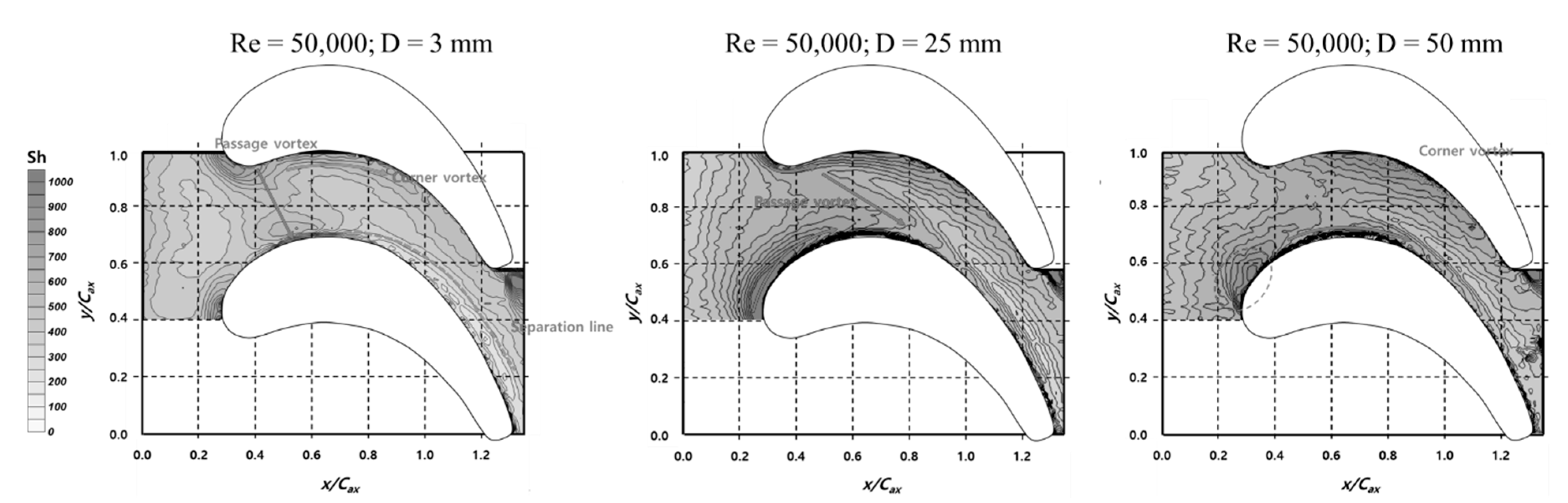
In the simulation, the first stage of the high-pressure turbine blade was considered. The dimensions of the blade are provided in Table 1. A previous work [30] was performed in ANSYS Fluent 19 R1 using the RANS equation to mitigate the computational time and cost using a sufficient number of grids. In this same aspect, the same number of grids was used for all cases; even the boundary layer thickness and Reynolds number varied. Finally, the result has a significant reduction in cost and time for obtaining a total of 38 low-fidelity data. The streamline contour for varied from the simulation is shown in Figure 3.
From the perspective of the GP surrogate, it is observed that the samples in Figure 1 are not distributed well. Therefore, the GP surrogate model depends on the correlation that relates to a distance between samples. Moreover, no samples are observed in the range of BL thickness between 30 and 50 mm. The unavailable samples could lead to large uncertainty in the GP prediction.
3. Results and Discussion
3.1. Low-Fidelity and High-Fidelity Surrogate Modeling for Heat Transfer Coefficient
As discussed previously, the most challenging part of constructing the GP surrogate is related to the aligned samples in this study. These aligned samples can cause difficulty in estimating the hyper-parameter in the GP surrogate. Therefore, the hyper-parameter is estimated manually based on the variation of LF and HF samples in each variable input direction. In the normalized input variable spaces, a normalized range of 1.0 to 3.0 is assigned to the hyper-parameter of LF-GP and HF-GP surrogates.
Figure 4 shows the distribution of averaged HTC by LF-GP surrogate using LF data. The LF-GP surrogate model shows a saturation trend in the direction and a monotonic behavior in the BL thickness direction. In general, the HTC is saturated as the BL thickness increases, which is referred to as a contradiction in Figure 4. The HTC variation with the BL thickness indicates that the grids near the wall should have refined well as the BL thickness changes so as to improve the accuracy of the simulation. As clearly mentioned earlier, the LF-GP surrogate model is built using data of the cheap simulation in this present study, the grid refinement near the wall is not required here as the BL thickness changes to minimize the computational time. Therefore, the error from the simulations increases inevitable in the BL thickness direction. As a result, the LF-GP surrogate model shows different behavior in the BL thickness direction.
Figure 5 shows the distribution of the averaged HTC by HF-GP surrogate using HF data, in which the same value of hyper-parameter that employed in the LF-GP surrogate is used. It is observed that the averaged HTC is linearly proportional to the . In contrast, the rate of averaged HTC is increased with the BL thickness up to 30 mm and then decreased with the BL thickness greater than 30 mm up to 50 mm. This tread in the BL thickness direction is contrary to the LF-GP surrogate model in Figure 4. Overall, the changing tendency of the HTC for variable inputs on the endwall by the HF-GP surrogate model is agreed well with the local high-fidelity data in Figure 5.
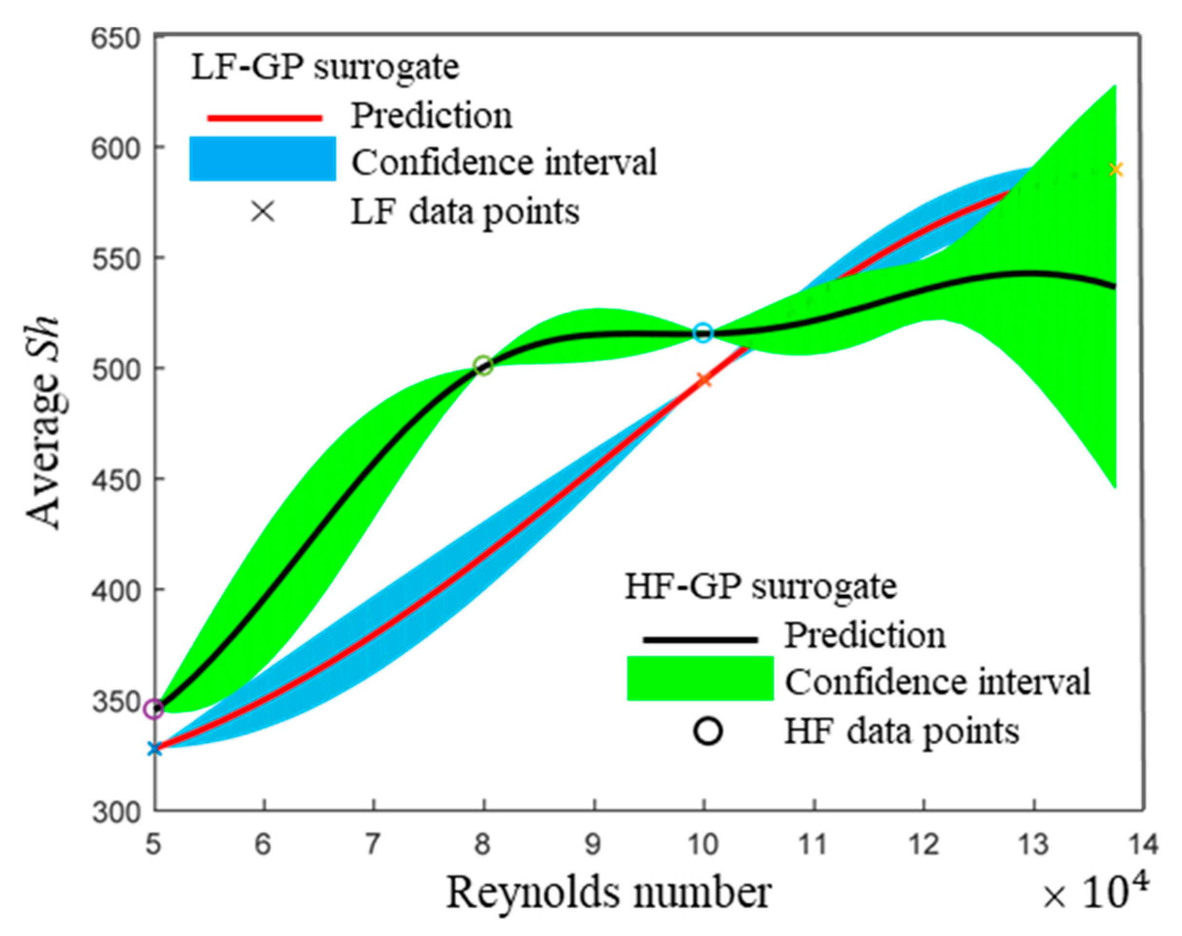
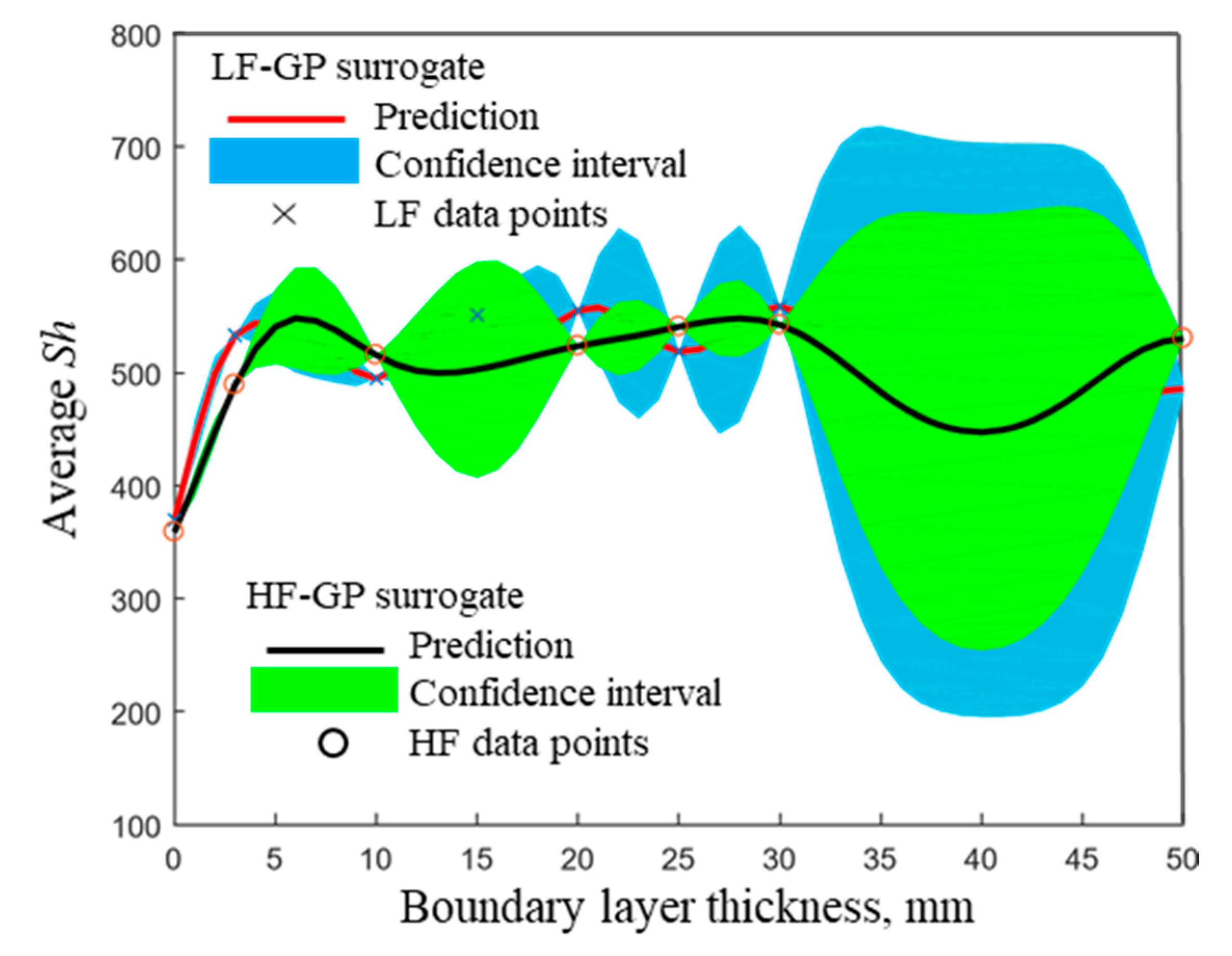
In order to compare further with LF and HF surrogates, one-dimensional cuts of two-dimensional surrogates are presented in Figure 6 and Figure 7. Figure 6 shows the LF and HF surrogate comparison with varied at a fixed BL thickness of 10 mm. The solid curve in red color indicates a prediction of the LF-GP surrogate, and the area in blue color indicates a 95% confidence interval. Since GP assumes that the data are exact, there is no uncertainty in the data points. The cross markers lying on the solid red curve are the three LG data points at the fixed BL thickness of 10 mm. Similarly, the solid curve in black color and the area in green color indicate the HF prediction and a 95% confidence interval of the HF-GP surrogate. The three HF data points lying on the black solid curve are shown in a circle shape. The comparison in Figure 6 reveals that the trend of HTC increases with , but the rate of increment varies significantly between the LF-GP and HF-GP surrogates.
Figure 7 shows the LF-GP and HF-GP surrogates with varied BL thickness at a fixed of 100,000. Note that the legends used in Figure 7 are the same as those in Figure 6. It is observed that the function is varied with the BL thickness at a high-frequency level. Therefore, the uncertainty (confidence interval) is obtained as larger than that variation with the case. It is worth mentioning that the uncertainty is significantly increased after 30 mm due to the unavailable data between 30 and 50 mm.
3.2. Evaluate the Accuracy of MFS
As already stated, the LF data are inexpensive but less reliable, and the HF data are precise but rather costly to obtain. The objective of the MFS model is to minimize the disadvantages and maximize the advantage of these two data sets. Therefore, the accuracy of MFS can decide that the MFS model is capable of practical applications. This subsection discusses the accuracy of MFS in predicting the averaged HTC on the endwall of the turbine blade.
To evaluate the accuracy of the MFS, the HF data must be compared with the value predicted by the MFS. The MFS is made by changing the number of HF data samples and then evaluating the accuracy by comparing the results with the HF data. The accuracy of the MFS can be expressed through the root-mean-square error (RMSE) between each MFS and HF data.
The HF data are randomly used to build the MFS. Among these, 0, 4, 6, 11, 14, 18, 21, or all high-fidelity data samples at a time are used to build each of the MFS. The RMSE values between the HF data and MFS models are shown in Table 2.
The LF surrogate model (0 high-fidelity data samples used, Figure 4) in Table 2 shows an RMSE of 32.4, which has an error rate of 7.2%. The error rate of the LF surrogate model is similar to the uncertainty of the experiment. It means that the LF surrogate model is a good model for predicting the HTC on the endwall of the turbine blade in the current design-parameter range. However, the changing tendency of the LF surrogate model is different from that in the HF surrogate model (Figure 5). As already mentioned, the HTC is increased in the LF-GP surrogate model in Figure 4 and is decreased with the BL thickness after 30 mm in the HF-GP surrogate model in Figure 5. It is observed in Figure 6 that the HTC is increased concave upwards up to of 100,000 (critical point), and after the critical point, it is increased concave downwards in the LF-GP surrogate model. In contrast, the HTC is increased concave downwards up to the critical point, and after this, it is merely constant in the HF-GP surrogate model. This comparison reveals that the different point of the HTC changing tendency is expected to increase the error in the HTC prediction by the LF-GP surrogate model when considering a range beyond the current design-parameter range.
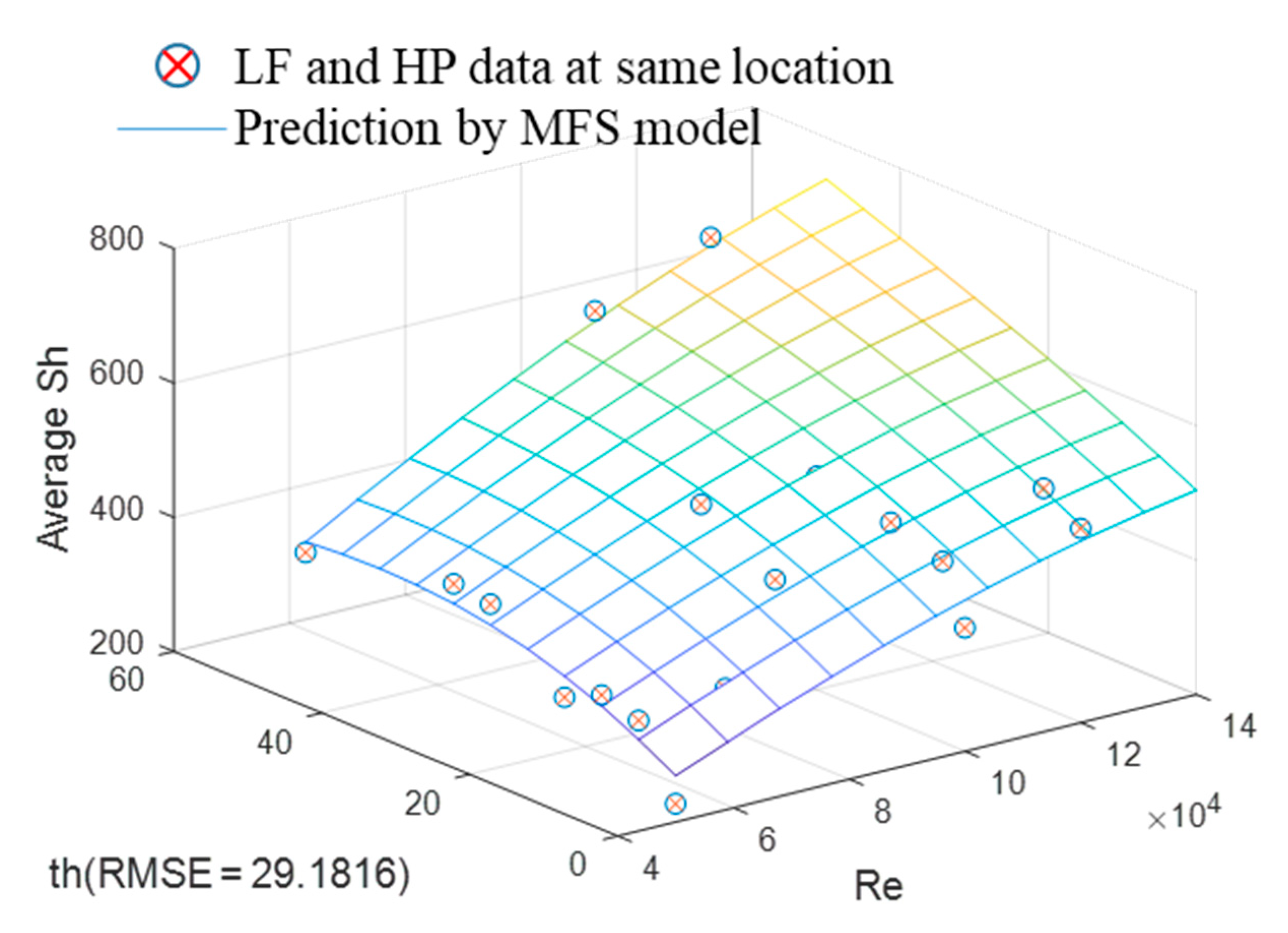
Using the LF surrogate and discrepancy surrogate, the MFS is built, and the HTC by the MFS is shown in Figure 8. The RMSEs of the HF surrogate in Figure 5 and MFS, including all HF data in Figure 8, are 29.74 and 29.18, respectively. Furthermore, the error rate is lesser than 6.5%, which is lower than the uncertainty of the naphthalene sublimation experiment. Therefore, a change in tendency of the two models is also similar within the current design-parameter range. This shows that the accuracy of the MFS, including all HF data for predicting the averaged HTC on the endwall of the turbine blade, has reached the level of experimental results.
With the local data difference between the HF surrogate model and MFS, including all HF data, the discrepancy surrogate is determined using Equation (2) and is shown in Figure 9. It is interesting that the discrepancy is significantly fluctuating without showing a monotonic trend. This may have happened because of significant noise in the test data or inconsistency in numerical analysis.
To compare further the LF and MFS, one-dimensional cuts of these two-dimensional surrogates are presented in Figure 10 and Figure 11. Figure 10 shows the prediction by the LF and MFS with varied at a fixed BL thickness of 10 mm. The black solid curve and the green areas are the averaged HTC predicted by MFS and 95% confidence intervals, respectively. Compared to the HF surrogate in Figure 6, the MFS shows more variations due to the effect of the LF surrogate.
Figure 11 shows the LF and MFS with varied BL thickness at a fixed of 100,000. It is observed that the function is varied with the BL thickness in a high-frequency level. Therefore, the uncertainty (confidence intervals) is obtained as larger than that variation with the case. It is worth mentioning that the uncertainty is significantly increased after 30 mm due to the unavailable data between 30 and 50 mm. As mentioned earlier, compared to the HF surrogate in Figure 7, the MFS shows more variations due to the effect of the LF surrogate.
The RMSE and error rate based on the number of HF data are shown in Figure 12. Found a remarkable change in the RMSE for the samples with more and few HF data. The samples of very few numbers of HF data have a higher RMSE than that the LF surrogate model. The RMSE of the MFS is decreased significantly as the number of HF data samples increased. Moreover, the samples of more than 18 HF data show that the MFS model’s error rate has reached slightly below the uncertainty of the experiment.
In general, the RMSE of the MFS is expected to be lesser than the RMSE of the LF surrogate model. In this present work, the RMSE calculated for the MFS of more than 18 HF data samples has similar or better than that for the LF surrogate model.
Through the present study, there is a key reason why a large number of HF data samples are required to improve the accuracy of the MFS. The reason is that the sample points in the design must be evenly distributed in the designed domain to make a good MFS model. However, the present work utilized the nonuniformly distributed point of the samples from our previous study [30]. Our previous work focused only on investigating the HT phenomenon on the endwall of the turbine blade, which is different from the sample distribution criteria for constructing the MFS model in this present work. As stated earlier, the larger interval between samples in the region of thickest BL and highest can cause a problem with the reliability interval of the predicted value of the surrogate model becoming very large in these regions. Therefore, to overcome these, more HF data are required for making MFS.
Compared to the result of the LF surrogate model, the MFS model has shown higher reliability in predicting the averaged HTC on the endwall of the turbine blade for the considered input range of the and BL thickness. As a consequence, it is possible to find a reliable result at any point of the desired domain and input range using the MFS model.
As discussed earlier, the samples based on the input variables are considered randomly and also aligned in a specified . However, the samples must consider in a wider range of desired locations. Additionally, still more HF data are required to build the MFS model, thereby to minimize the large confidence interval after = 100,000. There is a limitation of this present study.
This study suggests and proves that the method for making and evaluating the MFS using the data from our previous study [30], which from numerical analysis, experiment, and literature review. The utilization of the MFS model can be anticipated to reduce the time and cost of designing the turbine blades and cooling systems. In addition, this method of MFS configuration and evaluation is intended to be extended to other engineering design applications.
4. Conclusions
This paper focused on modeling the low-fidelity (LF), high-fidelity (HF) and multi-fidelity surrogates (MFS) model using LF and HF data to predict the averaged heat transfer coefficient (HTC) on the endwall of the turbine blade. In modeling the surrogates, the LF and HF data were used to build the LF and HF surrogate, respectively. The LF surrogate and discrepancy surrogate were used to build the MFS. In this present work, the input variables as Reynolds number () and boundary layer (BL) thickness were used. The LF surrogate showed a good prediction for the considered and BL thickness range except from 30 to 50 mm due to the unavailability of samples in the desired range. In addition, the prediction was saturated with the increase in the and had a monotonic behavior as the BL thickness increased. Similarly, the HF surrogate showed a good prediction for the same and BL thickness range due to the HF data. However, the confidence interval of the HF surrogate was found to be very high for the greater than 100,000. In addition, the prediction was linearly proportional to the and increased with BL thickness up to 30 mm then decreased after 30 mm due to no samples in the range of 30 to 50 mm.
The averaged HTC prediction by the MFS had a similar variation as the HF surrogate and better than the LF surrogate. In the MFS also, a large confidence interval was found for the higher BL thickness region due to the LF surrogate inclusion in building the MFS.
Since there were no test data to evaluate the accuracy of the MFS model, therefore the accuracy was evaluated using the HF data at a fixed BL thickness and . The root-mean-square error (RMSE) and error-rate of the MFS were large for fewer of HF data. The RMSE and error rate were decreased and also reached slightly below the experimental uncertainty for more HF data. This study concludes that the proposed MFS model helps to predict HTC for any other range of input variables. Thereby, MFS utilization in practical applications would be more useful for saving computational time and experimental cost.
Author Contributions
Conceptualization, N.-H.K. and J.S.P.; methodology, N.-H.K., W.C., J.S.P.; investigation, N.-H.K., W.C., J.S.P.; writing—original draft preparation, N.-H.K., W.C., J.S.P.; writing—review and editing, K.R., J.S.P.; project administration, J.S.P. All authors have read and agreed to the published version of the manuscript.
Funding
This research was supported by the Korean Electric Power Corporation (Grand number: R17XXA05-5) and Basic Science Research Program through the National Research Foundation of Korea (NRF) funded by the Ministry of Education (2019R1F1A1059573).
Institutional Review Board Statement
Not applicable.
Informed Consent Statement
Not applicable.
Conflicts of Interest
The authors declare no conflict of interest.
Nomenclature
| BL | Boundary layer |
| Chord length of the blade | |
| & | Corresponding function of low and high-fidelity |
| DoE | Design of experiments |
| Discrepancy surrogate | |
| GP | Gaussian process |
| HT | Heat transfer |
| HTC | Heat transfer coefficient () |
| HF | High-fidelity |
| HF-GP | High-fidelity-based Gaussian process |
| XH | High-fidelity dataset |
| High-fidelity model | |
| Thermal conductivity (here, air is fluid) | |
| LF | Low-fidelity |
| LF-GP | Low-fidelity-based Gaussian process |
| XL | Low-fidelity dataset |
| Low-fidelity model | |
| & | Low and high-fidelity surrogate |
| MFS | Multi-fidelity surrogate |
| Nusselt number | |
| Regression scalar | |
| Reynolds number | |
| RMSE | Root-mean-square error |
| Sherwood number |
References
- Yu, K.; Yang, X.; Yue, Z. Aerodynamic and heat transfer design optimization of internally cooling turbine blade based different surrogate model. Struct. Multidisc. Optim. 2011, 44, 75–83. [Google Scholar] [CrossRef]
- Choi, W.S.; Song, G.W.; Chang, S.Y.; Kim, B.S. Life assessment of gas turbine blade based on actual operation condition. Trans. Korean Soc. Mech. Eng. A 2014, 38, 1185–1191. [Google Scholar] [CrossRef]
- Mazur, Z.; Luna-Ramirez, A.; Juárez-Islas, J.A.; Campos-Amezcua, A. Failure analysis of a gas turbine blade made of inconel 738LC alloy. Eng. Fail. Anal. 2005, 12, 474–486. [Google Scholar] [CrossRef]
- Carter, T.J. Common failures in gas turbine blades. Eng. Fail. Anal. 2005, 12, 237–247. [Google Scholar] [CrossRef]
- Choi, W.S.; Chang, S.Y.; Kim, B.S.; Chen, Y.; Liu, Y.; Zhao, J.; Banerjee, A. The TMF life assessment of first-stage W501F turbine blade under different operating temperatures. In Proceedings of the ASME Turbo Expo 2015: Turbine Technical Conference and Exposition, Montreal, QC, Canada, 15–19 June 2015. ASME paper GT2015-43479. [Google Scholar]
- Han, J.C. Fundamental gas turbine heat transfer. J. Therm. Sci. Eng. Appl. 2013, 5, 021007. [Google Scholar] [CrossRef]
- Reyhani, M.R.; Alizadeh, M.; Fathi, A.; Khaledi, H. Turbine blade temperature calculation and life estimation—A sensitivity analysis. Propuls. Power Res. 2013, 2, 148–161. [Google Scholar] [CrossRef] [Green Version]
- Park, J.S.; Choi, W.S. Heat and mass transfer characteristics on the first-stage gas turbine blade under unsteady wake flow. Int. J. Therm. Sci. 2019, 138, 314–321. [Google Scholar] [CrossRef]
- Kandasamy, M.; Peri, D.; Ooi, S.K.; Carrica, P.; Stern, F.; Campana, E.F.; Osborne, P.; Cote, J.; Macdonald, N.; de Waal, N. Multi-Fidelity Optimization of a High-Speed Foil-Assisted Semi-Planning Catamaran for Low Wake. J. Mar. Sci. Technol. 2011, 16, 143–156. [Google Scholar] [CrossRef]
- Perdikaris, P.; Raissi, M.; Damianou, A.; Lawrence, N.D.; Karniadakis, G.E. Nonlinear information fusion algorithms for data-efficient multi-fidelity modelling. Proc. R. Soc. Lond. A Math. Phys. Eng. Sci. 2017, 473, 20160751. [Google Scholar] [CrossRef]
- Zou, Z.; Liu, J.; Zhang, W.; Wang, P. Shroud leakage flow models and a multi-dimensional coupling CFD (computational fluid dynamics) method for shrouded turbines. Energy 2016, 103, 410–429. [Google Scholar] [CrossRef]
- Minisci, E.; Vasile, M. Robust design of a reentry unmanned space vehicle by multifidelity evolution control. AIAA J. 2013, 51, 1284–1295. [Google Scholar] [CrossRef] [Green Version]
- Jonsson, I.M.; Leifsson, L.; Koziel, S.; Tesfahunegn, Y.A.; Bekasiewicz, A. Shape optimization of trawl-doors using variable-fidelity models and space mapping. Procedia Comput. Sci. 2015, 51, 905–913. [Google Scholar] [CrossRef] [Green Version]
- Forrester, A.I.; Bressloff, N.W.; Keane, A.J. Optimization using surrogate models and partially converged computational fluid dynamics simulations. Proc. R. Soc. Lond. A Math. Phys. Eng. Sci. 2006, 462, 2177–2204. [Google Scholar] [CrossRef]
- Kennedy, M.C.; O’Hagan, A. Predicting the output from a complex computer code when fast approximations are available. Biometrika 2000, 87, 1–13. [Google Scholar] [CrossRef] [Green Version]
- Qian, P.Z.; Wu, C.J. Bayesian hierarchical modeling for integrating low-accuracy and high-accuracy experiments. Technometrics 2008, 50, 192–204. [Google Scholar] [CrossRef]
- Balabanov, V.; Grossman, B.; Watson, L.; Mason, W.; Haftka, R. Multifidelity response surface model for HSCT wing bending material weight. In Proceedings of the 7th AIAA/USAF/NASA/ISSMO Symposium on Multidisciplinary Analysis and Optimization, St. Louis, MO, USA, 2–4 September 1998; pp. 778–788, Paper No. AIAA-98-4804. [Google Scholar]
- Mason, B.H.; Haftka, R.T.; Johnson, E.R.; Farley, G.L. Variable complexity design of composite fuselage frames by response surface techniques. Thin. Wall. Struct. 1998, 32, 235–261. [Google Scholar] [CrossRef]
- Knill, D.L.; Giunta, A.A.; Baker, C.A.; Grossman, B.; Mason, W.H.; Haftka, R.T.; Watson, L.T. Response surface models combining linear and euler aerodynamics for supersonic transport design. J. Aircr. 1999, 36, 75–86. [Google Scholar] [CrossRef]
- Viana, F.A.C. Surrogates Toolbox User’s Guide, 3rd ed.; University of Florida: Gainesville, FL, USA, 2011. [Google Scholar]
- Le Gratiet, L. Multi-fidelity gaussian process regression for computer experiments. Ph.D. Thesis, Université Paris-Diderot-Paris VII, Paris, France, 2013. [Google Scholar]
- Fischer, C.C.; Grandhi, R.V. A surrogate-based adjustment factor approach to multi-fidelity design optimization. In Proceedings of the 17th AIAA Non-Deterministic Approaches Conference, Kissimmee, FL, USA, 5–9 January 2015. Paper No. AIAA 2015-1375. [Google Scholar]
- Park, C.; Haftka, R.T.; Kim, N.H. Remarks on multi-fidelity surrogates. Struct. Multidiscip. Optim. 2017, 55, 1029–1050. [Google Scholar] [CrossRef]
- Campbell, K. Exploring Bayesian Model Calibration: A Guide to Intuition; Los Alamos Technical Report LAUR-02-7175; Los Alamos National Laboratory: Los Alamos, NM, USA, 2002. [Google Scholar]
- Swiler, L.P.; Trucano, T.G. Calibration under Uncertainty. SAND2005-14981498, Sandia National Laboratories (SNL-NM), Albuquerque, NM 87185-0370 (United States). 2005. Available online: https://prod-ng.sandia.gov/techlib-noauth/access-control.cgi/2005/051498.pdf (accessed on 1 August 2019).
- Forrester, A.I.; Sóbester, A.; Keane, A.J. Multi-fidelity optimization via surrogate modelling. Proc. R. Soc. A 2007, 463, 3251–3269. [Google Scholar] [CrossRef]
- Matsumura, T.; Haftka, R.T.; Kim, N.H. Accurate predictions from noisy data: Replication versus exploration with applications to structural failure. Struct. Multidiscip. Optim. 2015, 51, 23–40. [Google Scholar] [CrossRef]
- Higdon, D.; Kennedy, M.; Cavendish, J.C.; Cafeo, J.A.; Ryne, R.D. Combining field data and computer simulations for calibration and prediction. SIAM J. Sci. Comput. 2004, 26, 448–466. [Google Scholar] [CrossRef] [Green Version]
- Zhang, Y.; Kim, N.H.; Park, C.; Haftka, R.T. Multi-fidelity surrogate based on single linear regression. AIAA J. 2018, 56, 4944–4952. [Google Scholar] [CrossRef]
- Choi, W.; Jung, K.J.; Park, J.S. Characteristics of heat transfer on a turbine blade endwall under various inlet flow conditions. Exp. Heat Transf. 2020, 1–17. [Google Scholar] [CrossRef]
Figure 1.
Design of experiments for both low-fidelity (LF) and high-fidelity (HF) data.

Figure 2.
Mass transfer distribution on the endwall of the turbine blade from the naphthalene sublimation method [30].
Figure 2.
Mass transfer distribution on the endwall of the turbine blade from the naphthalene sublimation method [30].

Figure 3.
Streamline contour at the endwall from simulation [30].
Figure 3.
Streamline contour at the endwall from simulation [30].
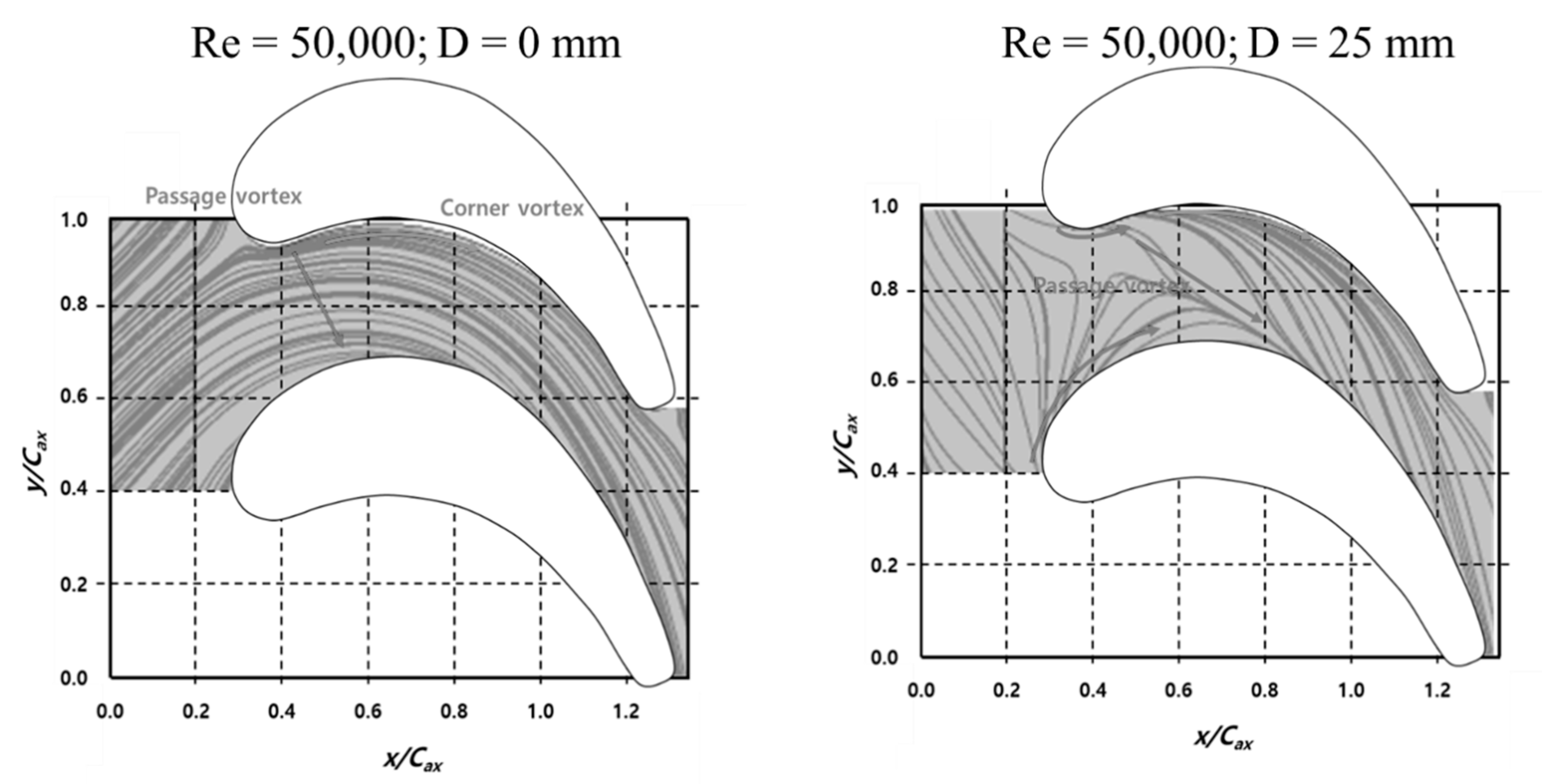
Figure 4.
Distribution of averaged heat transfer coefficient (HTC) by LF-Gaussian process (GP) surrogate using LF data.
Figure 4.
Distribution of averaged heat transfer coefficient (HTC) by LF-Gaussian process (GP) surrogate using LF data.
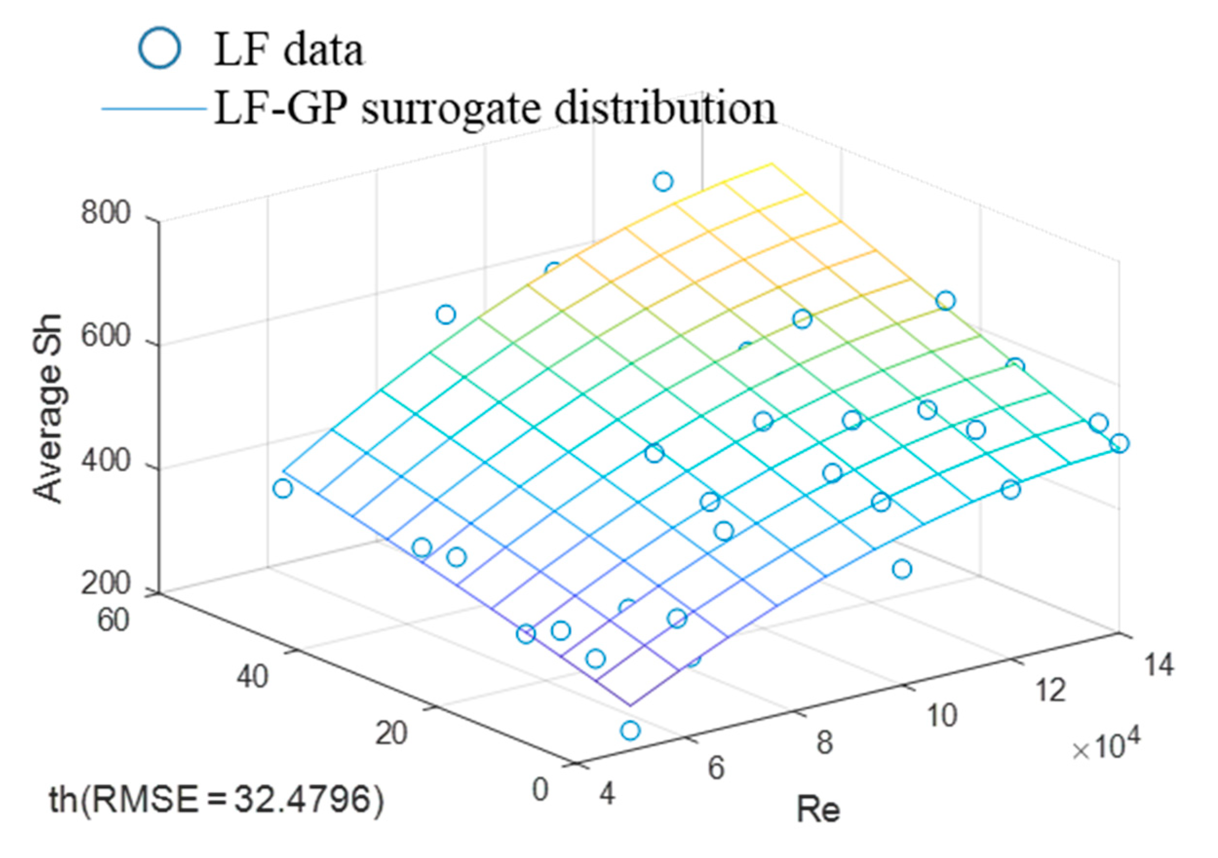
Figure 5.
Distribution of averaged HTC by HF-GP surrogate using HF data.
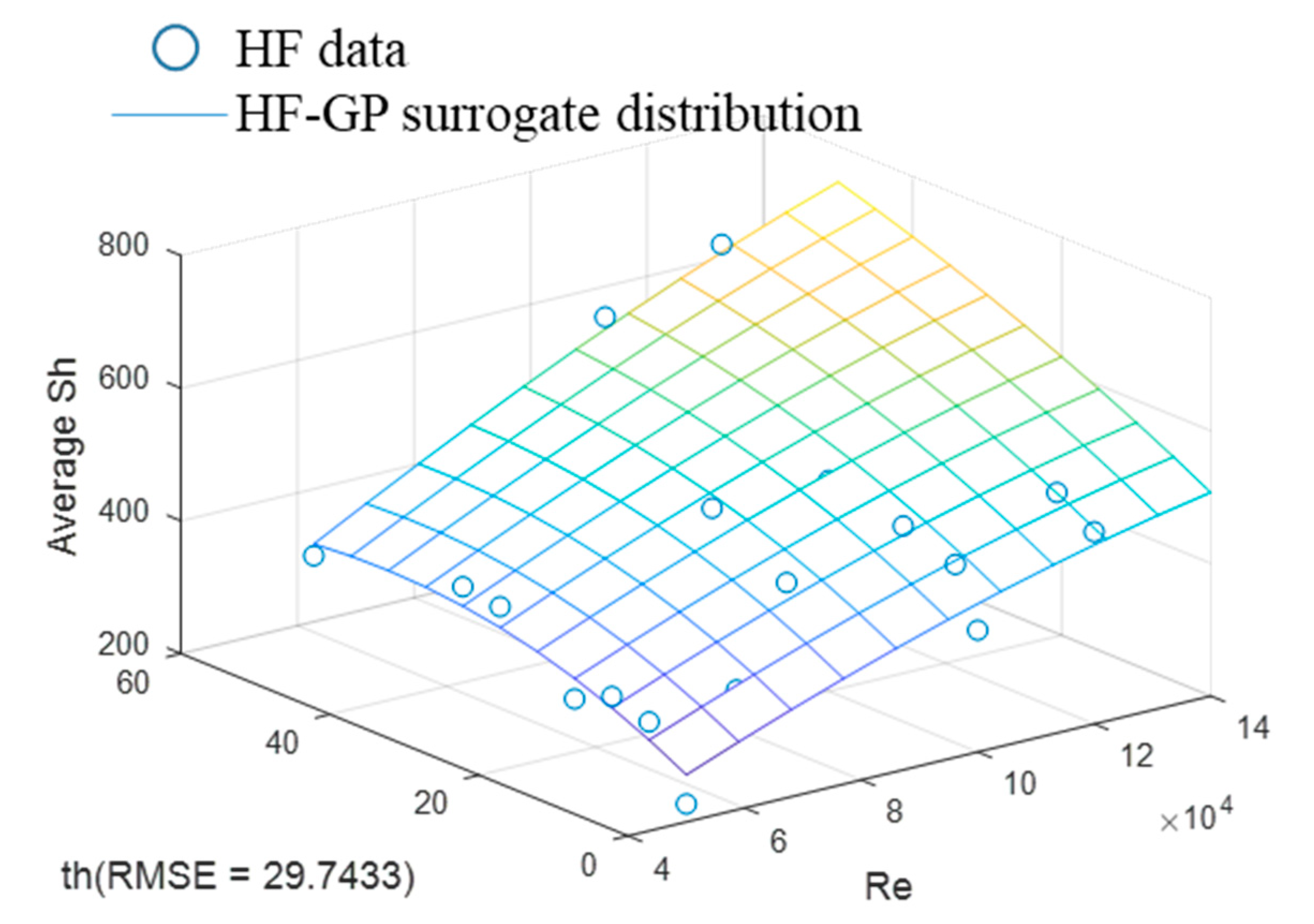
Figure 6.
1D projection of LF-GP and HF-GP surrogate for a fixed BL thickness of 10 mm.

Figure 7.
1D projection of LF-GP and HF-GP surrogate for a fixed of 100,000.

Figure 8.
Prediction of averaged HTC by MFS model.

Figure 9.
Discrepancy surrogate for the HTCs.
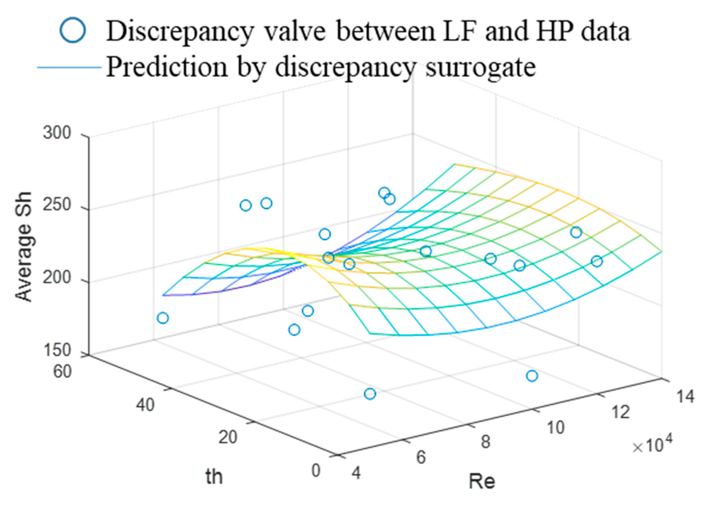
Figure 10.
1D projection of LF-GP surrogate and MFS for a fixed BL thickness of 10 mm.
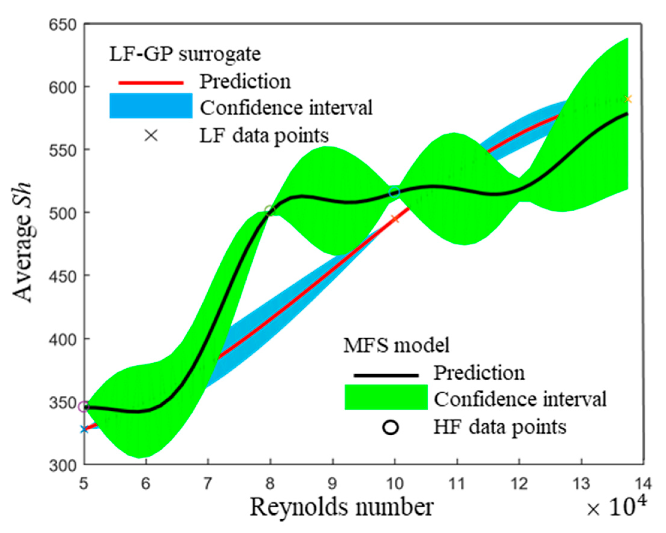
Figure 11.
1D projection of LF-GP surrogate and MFS for a fixed of 100,000.
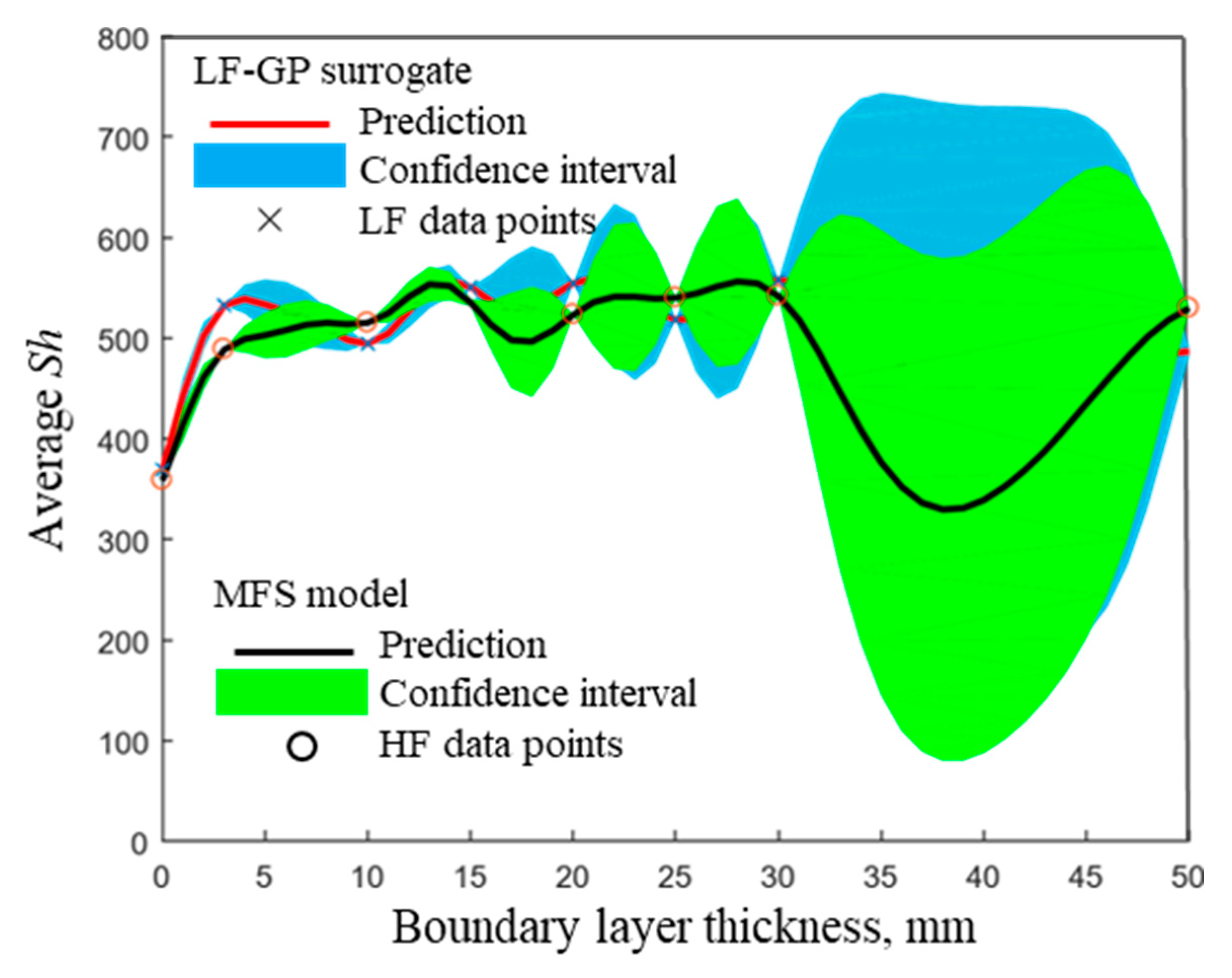
Figure 12.
Root-mean-square error (RMSE) and error rate in each MFS.


Table 1.
Dimensions of first stage turbine blade for simulation.
| Parameters | Values |
|---|---|
| Axial chord, mm | 114.62 |
| Inlet angle, deg | 46.23 |
| Leading-edge radius, mm | 17.07 |
| Pitch, mm | 80.0 |
| Tip clearance, mm | 6.0 |
Table 2.
RMSE value between the HF data and multi-fidelity surrogate (MFS) model (HF data average = 447.47).
Table 2.
RMSE value between the HF data and multi-fidelity surrogate (MFS) model (HF data average = 447.47).
| No of High-Fidelity Data | RMSE | Error Rate |
|---|---|---|
| 0 (low-fidelity surrogate) | 32.48 | 7.26 |
| 4 | 52.84 | 11.81 |
| 6 | 51.66 | 11.54 |
| 11 | 49.51 | 11.06 |
| 14 | 47.04 | 10.51 |
| 18 | 34.87 | 7.79 |
| 21 | 29.95 | 6.69 |
| 22 | 29.18 | 6.52 |
| High-fidelity surrogate | 29.95 | 6.69 |
Publisher’s Note: MDPI stays neutral with regard to jurisdictional claims in published maps and institutional affiliations. |
© 2021 by the authors. Licensee MDPI, Basel, Switzerland. This article is an open access article distributed under the terms and conditions of the Creative Commons Attribution (CC BY) license (http://creativecommons.org/licenses/by/4.0/).
Share and Cite
MDPI and ACS Style
Choi, W.; Radhakrishnan, K.; Kim, N.-H.; Park, J.S. Multi-Fidelity Surrogate Models for Predicting Averaged Heat Transfer Coefficients on Endwall of Turbine Blades. Energies 2021, 14, 482. https://doi.org/10.3390/en14020482
AMA Style
Choi W, Radhakrishnan K, Kim N-H, Park JS. Multi-Fidelity Surrogate Models for Predicting Averaged Heat Transfer Coefficients on Endwall of Turbine Blades. Energies. 2021; 14(2):482. https://doi.org/10.3390/en14020482
Chicago/Turabian StyleChoi, Woosung, Kanmaniraja Radhakrishnan, Nam-Ho Kim, and Jun Su Park. 2021. "Multi-Fidelity Surrogate Models for Predicting Averaged Heat Transfer Coefficients on Endwall of Turbine Blades" Energies 14, no. 2: 482. https://doi.org/10.3390/en14020482
Note that from the first issue of 2016, this journal uses article numbers instead of page numbers. See further details here.