A Multiscale Electricity Price Forecasting Model Based on Tensor Fusion and Deep Learning

Abstract

The price of electricity is an important factor in the electricity market. Accurate electricity price forecasting (EPF) is very important to all competing electricity market parties. Decision-making in the electricity market is highly dependent on electricity prices, making an EPF model an important part of the orderly and efficient operation of the electricity market. Especially during the COVID-19 pandemic, the prices of raw materials for electricity production, such as coal, have risen sharply. Forecasting electricity prices has become particularly important. Currently, existing EPF prediction models face two main challenges: First, how to integrate multiscale electricity price data to obtain a higher prediction accuracy. Second, how to solve the problem of data noise caused by the fusion of EPF samples and multiscale data. To solve the above problems, we innovatively propose a tensor decomposition method to integrate multiscale electricity price data and use $L_1$ regularization and wavelet transform to remove data noise. In general, this paper proposes a deep learning EPF prediction model, named the WT_TDLSTM model, based on tensor decomposition, a wavelet transform, and long short-term memory (LSTM). Among them, the LSTM method is used to predict electricity prices. We conducted experiments on three datasets. The experimental results of three data prove that the WT_TDLSTM model is better than the compared EPF model. The indicators of MSE and RMSE are 33.65–99.97% better than the comparison model. We believe that the WT_TDLSTM model is a good supplement to the EPF model.

1. Introduction

The price of electricity is an important factor in the electricity market [1]. Accurate electricity price forecasting (EPF) is very important to all parties in power market competition [2,3,4]. Decision-making in the electricity market is highly dependent on the electricity price, making an EPF model an important part of the orderly and efficient operation of the electricity market. EPF has a certain periodicity, as well as a high degree of randomness and time-varying characteristics [5]. Therefore, building a model for forecasting electricity prices is a very challenging task. The accuracy of EPF in the power market affects the efficiency and rationality of energy resource optimization [6]. Especially for enterprises, it is important to accurately predict the price of electricity to control their production costs. In addition, accurate electricity price forecasting can achieve a balance between the electricity supply and demand, which is conducive to stable electricity market operation. At present, with the global pandemic of COVID-19, the cost of raw materials in the power industry have risen sharply [7]. This exacerbates the fluctuation of electricity prices and further makes electricity price forecasting more important.

Existing EPF methods can be divided into three categories, namely, physical methods, statistical methods, and machine learning methods (Figure 1). Physical methods are based on safety constrained unit commitment (SCUC) and safety constrained economic dispatch (SCED) models to simulate the day-to-day power market situation based on boundary conditions and physical theory [8,9]. Although physical methods are effective from the perspective of predictive logic, their main problem is that the SCUC and SCED models require a large amount of real-time operating data, such as line transmission capacity, electricity load, and competitors’ bids, which leads to very complicated calculations. Statistical methods aim to use curve fitting to reveal the dynamic trends between historical electricity price series. These methods have the advantages of high-speed performance, simple modelling and convenience. Statistical models include the autoregressive moving average (ARMA) [10,11], generalized autoregressive conditional heteroscedasticity (GARCH) [12], and chaos theory [13]. Machine learning methods can be roughly divided into two categories: shallow learning models and deep learning models [14,15]. Shallow learning models are based on the principle of error minimization and generally have better performance than physical and statistical methods [16]. Due to their remarkable ability to extract features, they have been one of the most commonly used methods for electricity price forecasting. Shallow learning models include support vector regression (SVR) [17], artificial neural networks (ANNs) [18], and regression trees [19]. After 2021, some researchers have also proposed a kernel-based extreme learning machine power price prediction model [20,21]. Recently, with the development of deep learning, electricity price prediction models based on deep learning have been continuously proposed, including BP, CNN, RNN, etc. [22,23,24]. Recently, the LSTM-based electricity price prediction method has received widespread attention because of its excellent performance. For example, Huang et al. proposed an LSTM-based electricity price prediction model [25]. Memarzadeh et al. proposed an improved LSTM model named LSTM-NN to achieve a better short-term electricity price prediction model [26].

However, the existing EPF machine learning prediction models still faces two main limitations. First, most of the existing EPF models are single-scale models. Existing research has proven that compared with a single-scale training model, a multiscale EPF model can obtain increasingly comprehensive data features, and thus, it is possible to achieve better prediction accuracy [27]. The feature length of multiscale time series data is inconsistent and contains noise. This leads to difficulty in establishing an end-to-end prediction model. The second limitation is that the existing data denoising methods are still not perfect, and the results of the model still have room for improvement. Electricity price data have high dimensionality and high noise characteristics. Especially after the data are segmented using a sliding window, the sample quality problem of each sliding window becomes more prominent. In addition, the multiscale fusion process of a model may bring additional noise problems. Therefore, it is difficult for researchers to obtain an ideal model based on all samples and features.

In this paper, we propose an EPF prediction model based on tensor decomposition, wavelet transform and long short-term memory. The method of using tensors for feature fusion has been widely used in various artificial intelligence fields and has achieved good results [28,29,30]. This paper proposes a tensor decomposition method based on $L_1$ to fuse multiscale power data. Among them, the $L_1$ regularizer is used to solve the data noise problem caused by the fusion of the EPF sample itself and the multiscale tensor. We also used the wavelet transform method for data denoising. A wavelet transform (WT) is a new transform analysis method that inherits and develops the idea of localization of a short-time Fourier transform while overcoming the shortcomings of the window size not changing with frequency by using a WT’s “time-frequency” window that changes with frequency. This method has been widely used in the denoising of time series data [31,32,33]. Finally, we use a long short-term memory (LSTM) model on the processed features for data prediction.

The contributions of this study can be summarized as follows:

• We innovatively propose a tensor decomposition method based on $L_1$ regularons, which can effectively fuse multiscale electricity price data and remove the noise generated during data fusion.
• To the best of our knowledge, WT_TDLSTM is the first multiscale integration model that incorporates wavelet transform and tensor fusion into a computational framework.
• The experimental results show that, compared with a neural network model that does not perform denoising and fusion of multiscale data, the prediction performance of the WT_TDLSTM model achieves significantly better results.

2. Datasets and Methods

2.1. Datasets

In this study, the monthly electricity price sample we adopted for validating the priority of the proposed method was selected from the Energy Information Administration (EIA) (U.S.) (https://www.eia.gov accessed: October 2021) and included residential, commercial, and industrial monthly electricity price samples (see

Table 1. Statistical description of three types of electricity price data samples in this study.

Sample	Statistic	Value
residential	Length	245
	Max	13.76
	Min	7.13
	Average	11.28
commercial	Length	245
	Max	11.93
	Min	7.25
	Average	9.78
industrial	Length	245
	Max	8.15
	Min	4.71
	Average	6.38

). The number of samples for which residential, commercial, and industrial monthly electricity prices are all 245 (January 2001/May 2021). Before training, we preprocess the data of the residential monthly electricity prices as follows. First, we segment the data samples. For example, electricity price data from January to November 2001 are used to predict electricity prices in December 2001, and electricity price data from February to December 2001 are used to predict electricity prices in January 2002. Based on the above preprocessing strategy, we developed a new dataset with 234 samples. Next, we divide these data into multiple scales, and the time lengths are 12, 8, and 5 months.

2.2. Tensor Fusion

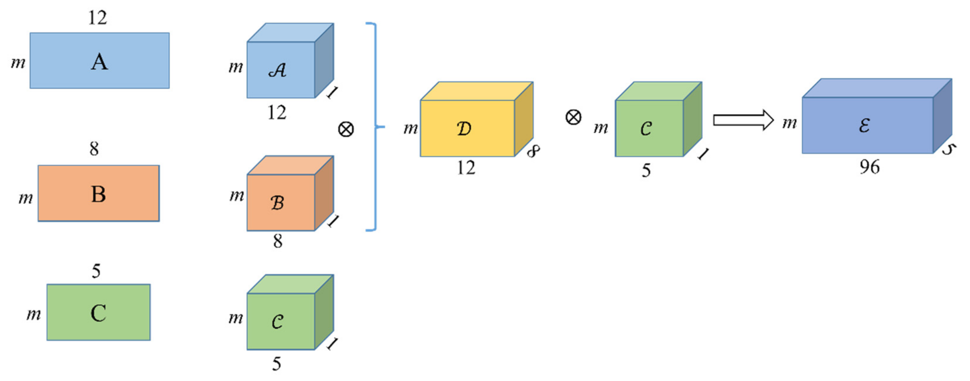
In this paper, we divide the electricity price data on multiple scales and obtain a matrix $A\in {ℝ}^{m\times 12}$ with a scale length of 12, a matrix $B\in {ℝ}^{m\times 8}$ with a scale length of 8, and a matrix $C\in {ℝ}^{m\times 5}$ with a scale length of 5. To perform tensor fusion on multiscale data, we transform matrices A, B and C into tensors $\mathcal{A}\in {ℝ}^{m\times 12\times 1}$, $\mathcal{B}\in {ℝ}^{m\times 1\times 8}$ and $\mathcal{C}\in {ℝ}^{m\times 1\times 5}$. Figure 2 shows the process of tensor fusion for multiscale data. Next, we briefly describe the tensor fusion strategy, and the result is shown using the following formula:

$$\mathcal{D}=\mathcal{A} \otimes \mathcal{B}.$$

(1)

where $\mathcal{D}\in {ℝ}^{m\times 12\times 8}$ and $\otimes$ denote the matrix multiplication of two dimensions of the tensor.

To be able to further merge with the tensor $\mathcal{C}$, we convert the size of $\mathcal{D}$ to $m\times 96\times 1$ and use the following formula:

$$\mathcal{E}=\mathcal{D} \otimes \mathcal{C}.$$

(2)

where $\mathcal{E}\in {ℝ}^{m\times 96\times 5}$ and is our final multiscale fusion tensor.

2.3. Tensor Decomposition

2.3.1. Tucker Decomposition

We can regard Tucker tensor decomposition as a form of higher-order PCA [34]. Tucker tensor decomposition factorizes $\mathcal{X}$ into N factor matrices and the core tensor that constitutes a compressed version of $\mathcal{X}$. If we assume that $\mathcal{X}$ is a tensor of size $I_1\times I_2\times \cdots \times I_N$, then the optimization problem to be solved to calculate the Tucker decomposition is

$$min\Vert \mathcal{X}-⟦\mathcal{G};U_1,U_2,\cdots ,U_N⟧\Vert {}_F^2.$$

(3)

we can easily find an exact Tucker decomposition of rank $\left(R_1,R_2,\cdots ,R_N\right)$, where $R_n\le rank\left(\mathcal{X}\right)$, $\mathcal{G}\in {ℝ}^{R_1\times R_2\times \cdots \times R_N}$; factor matrices $U_n\in {ℝ}^{I_n\times R_n}$ and column-wise orthogonal for $n=1, 2,\cdots ,N$, $\Vert ·\Vert {}_F^2.$ denotes the L2 (or Frobenius) norm.

If the solution of Equation (3) is at the optimal solution, then the core tensor $\mathcal{G}$ must satisfy

$$\mathcal{G}=\mathcal{X}{\times }_1{U}_1^T{\times }_2{U}_2^T\cdots {\times }_N{U}_N^T.$$

(4)

Substituting Equation (4) into Equation (3), the optimization goal can be recast as a series of subproblems involving the following maximization problem:

$$max\Vert \mathcal{X}{\times }_1{U}_1^T{\times }_2{U}_2^T\cdots {\times }_N{U}_N^T\Vert {}_F^2.$$

(5)

We can use the alternating least squares (ALS) method to solve (5); if $U_n^{*}$ is a solution to (5), then

$${\mathcal{G}}^{*}=\mathcal{X}{\times }_1{U}_1^{*}{}^T{\times }_2{U}_2^{*}{}^T\cdots {\times }_N{U}_N^{*}{}^T.$$

(6)

${\mathcal{G}}^{*}$ is the corresponding Tucker core of $\mathcal{X}$, and $\mathcal{X}$ is “low-rank” approximated by

$$\widehat{\mathcal{X}}={\mathcal{G}}^{*}{\times }_1{U}_1^{*}{\times }_2{U}_2^{*}\cdots {\times }_N{U}_N^{*}=\mathcal{X}{\times }_1{U}_1^{*}{U}_1^{*}{}^T{\times }_2{U}_2^{*}{U}_2^{*}{}^T\cdots {\times }_N{U}_N^{*}{U}_N^{*}{}^T.$$

(7)

where $\widehat{\mathcal{X}}$ is the reconstructed tensor. The exact solution to (5) remains unknown and can be commonly approximated by means of HOSVD algorithms based on the ALS method.

2.3.2. L1-HOSVD

As noise will inevitably be introduced in the process of tensor fusion of multiscale data, we use the L1-HOSVD [35] decomposition method based on Tucker decomposition to denoise the fused tensor. L1-HOSVD derives by simply replacing the L2-norm in (5) by the corruption resistant L1-norm as follows:

$$max\Vert \mathcal{X}{\times }_1{U}_1^T{\times }_2{U}_2^T\cdots {\times }_N{U}_N^T\Vert {}_1.$$

(8)

We find that to solve Equation (8), it is necessary to continuously iteratively solve the factor matrix $U_n$. For the solution of the factor matrix $U_n$, the objective function Equation (9) needs to be optimized:

$$U_n=argmax \Vert U^T{\mathcal{X}}_{\left(n\right)}\Vert {}_1.$$

(9)

where $U\in {ℝ}^{I_n\times R_n}$,$U^{T}U={\mathbb{I}}_{R_n}$; ${\mathbb{I}}_{R^n}$ refers to the identity matrix of size $R_n\times R_n$. ${\mathcal{X}}_{\left(n\right)}$ are the mode-n matricization of tensor $\mathcal{X}$.

We pursue the solution to (9) approximately by means of a fixed-point iteration (FPI) algorithm. According to [36], we can obtain the solution process as follows:

$$max\Vert U^T{\mathcal{X}}_{\left(n\right)}\Vert {}_1=maxTr\left(U^T{\mathcal{X}}_{\left(n\right)}\mathit{B}\right)$$

(10)

where $\mathit{B}\in {\left\{\pm 1\right\}}^{P_n\times R_n}$ is an indicator variable. We develop an alternate updating rule to optimize the objective function of Equation (10) as follows:

$$\begin{array}{c}{\mathit{B}}_{n,t}=\underset{\mathit{B}\in {\left\{\pm 1\right\}}^{P_n\times R_n}}{argmax}Tr\left(U_{n,t-1}^T{\mathcal{X}}_{\left(n\right)}\mathit{B}\right)\\ =sgn\left({\mathcal{X}}_{\left(n\right)}^T{U}_{n,t-1}\right).\end{array}$$

(11)

$$\begin{array}{c}{U}_{n,t}=\underset{U\in {ℝ}^{I_n\times R_n},U^{T}U={\mathbb{I}}_{R_n}}{argmax}Tr\left(U^T{\mathcal{X}}_{\left(n\right)}{\mathit{B}}_{n,t}\right)\\ =\mathsf{\Phi }\left({\mathcal{X}}_{\left(n\right)}{\mathit{B}}_{n,t}\right).\end{array}$$

(12)

where $sgn\left(·\right)$ returns the ±1 signs of the entries of its argument ($sgn\left(0\right)=1$), and $t$ refers to the t-th iteration. Moreover, it holds that $\mathsf{\Phi }\left(H\right)=\underset{U\in {ℝ}^{m\times n}}{argmax}Tr\left(U^{T}H\right)=\underset{U\in {ℝ}^{m\times n}}{argmin}\Vert U-H\Vert {}_F^2$ by the Procrustes Theorem [37].

To simplify the updating process, we integrate Equations (11) and (12) as follows:

$$U_{n,t}=\mathsf{\Phi }\left({\mathcal{X}}_{\left(n\right)}sgn\left({\mathcal{X}}_{\left(n\right)}^T{U}_{n,t-1}\right)\right).$$

(13)

Finally, we randomly initialize the factor matrices $U_{n,1}$ and update the factor matrices by Equation (13) until the model converges. In this paper, we replace tensor $\mathcal{X}$ with multiscale fusion third-order tensor $\mathcal{E}\in {ℝ}^{m\times 96\times 5}$ for denoising.

2.4. Wavelet Transform

A wavelet transform is a new transform analysis method that inherits and develops the idea of the localization of a short-time Fourier transform and simultaneously overcomes the shortcomings of the window size not changing with frequency by using a “time-frequency” window that changes with frequency. This makes it an ideal tool for signal time-frequency analysis and processing.

The main feature of a WT is that it can fully highlight the characteristics of certain aspects of a problem through transformation and can localize the analysis of time (space) frequency. It gradually refines the signal (function) at multiple scales through expansion and translation operations and finally achieves time subdivision at high frequencies and frequency subdivision at low frequencies. It can automatically adapt to the requirements of time-frequency signal analysis so that it can focus on any detail of the signal.

The basic formula of a wavelet transform is as follows:

$$\mathrm{WT}\left(\mathsf{\alpha },\mathsf{\tau }\right)=\frac{1}{\sqrt{\mathsf{\alpha }}}{{\displaystyle \int }}_{-\infty }^{\infty }f\left(t\right)\times \psi \left(\frac{t-\mathsf{\tau }}{\mathsf{\alpha }}\right)dt.$$

(14)

where $\mathsf{\alpha }$ is the scale and $\mathsf{\tau }$ is the displacement.

2.5. Long Short-Term Memory

A long short-term memory network is a special type of RNN that can learn long-term dependence information. The LSTM method was proposed by Hochreiter and Schmidhuber (1997) [38] and was recently improved. LSTM has achieved considerable success and has been widely used [39,40,41].

The key to LSTM is the state of the cell. The first step in the LSTM method is to decide what information the model will discard from a cell state. This decision is made through a layer called the forget door. Suppose the cell state after the last cycle is $C_{t-1}$. The gate will read the result $h_t$ of the last cycle of the model and the current input $x_t$ and output a value between 0 and 1 for each cell state parameter in $C_{t-1}$, where 1 means “completely reserved” and 0 means “completely discarded”.

We define a function $f_t$ to determine the information discarded by the model in this cycle:

$$f_t=\sigma \left(W_t\left[h_{t-1},x_t\right]+b_f\right).$$

(15)

where $\sigma$ represents an activation function and $W_t$ and $b_f$ are the weight and bias information, respectively.

The next step is to determine what new information is stored in the cell state. There are two parts here. First, the input gate layer determines the value that the model needs to be updated. Second, a new candidate variable ${\tilde{C}}_t$ is created, which is added to the state.

$$i_t=\sigma \left(W_i\left[h_{t-1},x_t\right]+b_i\right),$$

(16)

$${\tilde{C}}_t=\tan \mathrm{h}\left(W_C\left[h_{t-1},x_t\right]+b_C\right).$$

(17)

Finally, the cell state is updated using the following formula:

$$C_t=f_t\times C_{t-1}+i_t\times {\tilde{C}}_t.$$

(18)

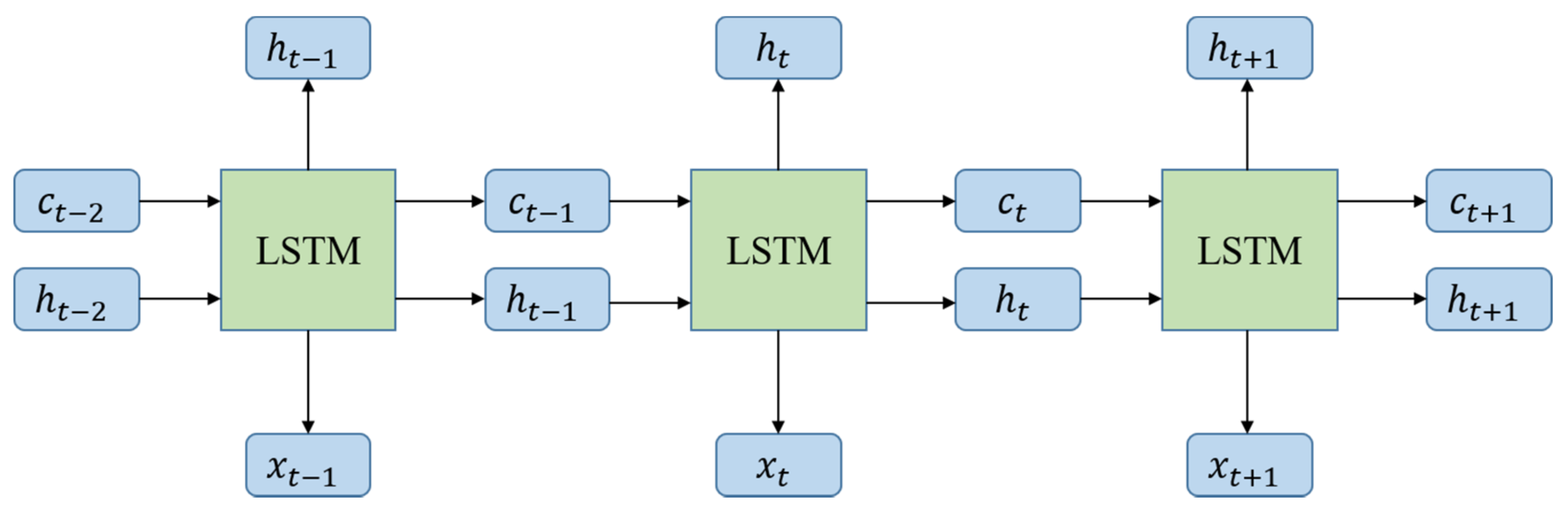
Although the LSTM maintains a similar structure to the standard RNN, the cell composition is different. The LSTM introduced above can effectively solve the problem of gradient disappearance and gradient explosion in the RNN training process because of its unique structure. Figure 3 illustrates the schematic diagram of LSTM network training.

In this paper, we construct an LSTM deep learning model with two hidden layers, the activation functions are sigmoid and tanh, and the hidden layer neurons are set to 5.

2.6. WT_TDLSTM

To overcome the influence of noise caused by multiscale data fusion and establish a high-precision regression model, we innovatively combine wavelet transform and tensor decomposition with LSTM (see Figure 4). The specific workflow is as follows:

Step 1: We divide the electricity price data into multiscale and use a wavelet transform to denoise data of different scales;

Step 2: We integrate multiscale data into a tensor and use L1-HOSVD based on Tucker decomposition to decompose the tensor to obtain factor matrices of different dimensions and the compressed version of the core tensor;

Step 3: We use the factor matrices and the core tensor to obtain the reconstructed tensor, which is the denoised tensor. Then, the denoised tensor is converted to a matrix, and the matrix is normalized;

Step 4: Based on the normalized matrix, we take advantage of the LSTM model for the final electricity price prediction.

3. Results

In this section, we first show how to preprocess residential, commercial, and industrial monthly electricity price samples. Then, we introduce the evaluation metrics of the model and the adjustment of hyperparameters. Finally, we compare and analyze the performance of our model with other models.

3.1. Data Preprocessing

Considering that activation functions such as ReLu in the neural network will map all negative values to 0, all sample data are normalized before network training to reduce training time and improve the training effect. In this paper, we use the minmax normalization method to preprocess the electricity price data. The normalization formulation is as follows:

$$X^{*}=\frac{X-min\left(X\right)}{max\left(X\right)-min\left(X\right)}.$$

(19)

where $X^{*}$ denotes the result of normalizing the input data and $max\left(X\right)$ and $min\left(X\right)$ refer to the maximum and minimum values of the input data, respectively.

3.2. Performance Metrics

In this study, four evaluation indicators, the mean squared error (MSE), root mean square error (RMSE), and mean absolute error (MAE), are applied in this subsection. The calculations of these indices are shown in Equations (20)–(22).

$$\mathrm{MSE}=\frac{1}{n}{\displaystyle }\sum _{i=1}^n{\left(y_i-{\widehat{y}}_i\right)}^2,$$

(20)

$$\mathrm{RMSE}=\sqrt{\frac{1}{n}{\displaystyle \sum }_{i=1}^n{\left(y_i-{\widehat{y}}_i\right)}^2},$$

(21)

$$\mathrm{MAE}=\frac{1}{n}{\displaystyle \sum }_{i=1}^n\left|y_i-{\widehat{y}}_i\right|.$$

(22)

3.3. The Effects of the Hyperparameters

In our model, some hyperparameters have different effects on the experimental performance. We take the residential monthly electricity price dataset as an example to show the process of adjusting hyperparameters. Here, we focus on two specific hyperparameters, i.e., the number of neurons and the learning rate λ in the WT_TDLSTM model. To better evaluate the influence of hyperparameters on the model, we use the MSE and MAE to select hyperparameters. First, we fix the value of the learning rate at 0.001 and search for the optimal values of the other parameters. Then, we vary the number of neurons in the hidden layer within {3, 5, 10, 20} to find the best parameter. From

Table 2. Performance of the WT_TDLSTM model with different values of neurons in the hidden layers on the residential monthly electricity price dataset.

	MSE	MAE
3	0.002130	0.034939
5	0.001973	0.033888
10	0.002026	0.034724
20	0.003464	0.047668

, we can see that when the number of hidden neurons is 5 in the WT_TDLSTM model, the values of MSE and MAE are the smallest (MSE = 0.001973, MAE = 0.033888). Finally, after the above hyperparameters are determined, we can change the value of the learning rate within {1, 0.1, 0.01, 0.001, 0.0001} to find the optimal parameter. In Figure 5, we find that when the learning rate is 0.001, the values of MSE and MAE are the smallest. It is worth noting that commercial and industrial monthly electricity price datasets in this paper should also use the above steps for hyperparameter selection.

3.4. The Results on the Dataset

Table 3. Five randomized experimental average results of all the models on the residential monthly electricity price dataset.

Model	MSE	RMSE	MAE
BP	0.113129	0.012798	0.281345
CNN	0.006854	4.697257 × 10−5	0.071783
RNN	0.104034	0.010823	0.239140
LSTM	0.101310	0.010264	0.238800
LSTM-NN	0.091435	0.008360	0.225945
WT_TDLSTM	0.001985	3.940309 × 10−6	0.035024

,

Table 4. Five randomized experimental average results of all the models on the commercial monthly electricity price dataset.

Model	MSE	RMSE	MAE
BP	0.120919	0.014621	0.277841
CNN	0.125190	0.015673	0.327035
RNN	0.203747	0.041513	0.394502
LSTM	0.307191	0.094366	0.445847
LSTM-NN	0.253752	0.064390	0.437149
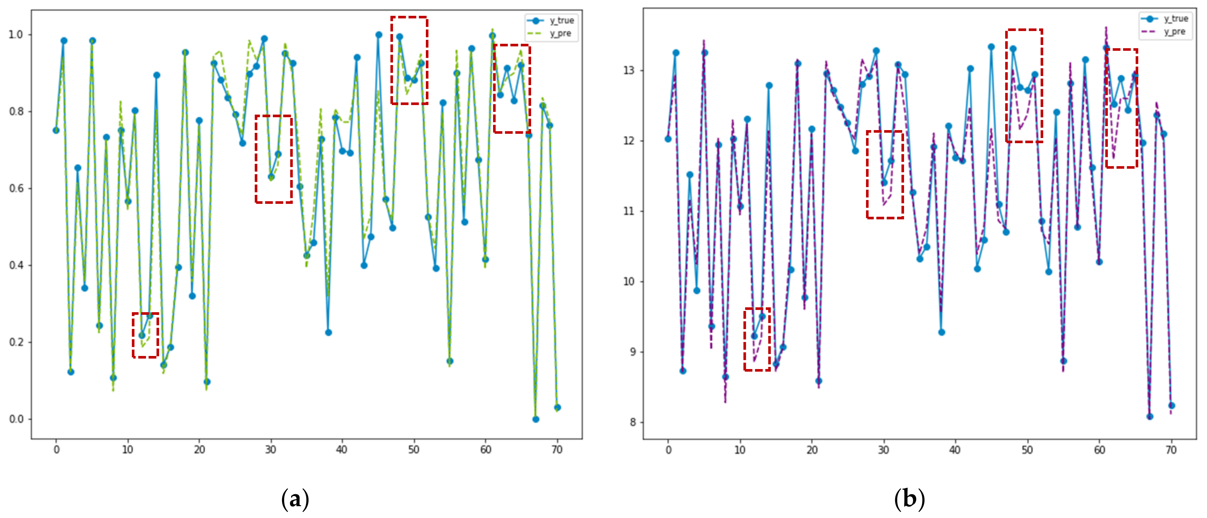
WT_TDLSTM	0.080231	0.006437	0.263357

and

Table 5. Five randomized experimental average results of all the models on the industrial monthly electricity price dataset.

Model	MSE	RMSE	MAE
BP	0.085263	0.007270	0.217354
CNN	0.091712	0.008411	0.255854
RNN	0.088921	0.007907	0.229501
LSTM	0.148374	0.022015	0.296279
LSTM-NN	0.124202	0.015426	0.283735
WT_TDLSTM	0.050549	0.002555	0.207223

show the prediction performance of different models on the residential, commercial and industrial monthly electricity price datasets, respectively. In this paper, we choose five deep learning-based models as our baseline models, including BP, CNN, RNN, LSTM, and LSTM-NN. For our model, we can see that the average values of the MSE, RMSE, and MAE in five randomized experiments are 0.001985, 3.940309 × 10⁻⁶, and 0.035024, respectively, as shown in Table 3. The values of the evaluation metrics of the WT_TDLSTM model are 98.25%, 99.97%, and 87.55% better than those of the BP model; 71.04%, 91.61%, and 51.21% better than those of the CNN model; 98.09%, 99.96%, and 85.35% better than those of the RNN model; 98.04%, 99.96%, and 85.33% better than those of the LSTM model; and 97.83%, 99.95%, and 84.50% better than those of the LSTM-NN model. Similarly, from Table 4 and Table 5, we can also find that the average values of MSE, RMSE, and MAE of the WT_TDLSTM model are significantly better than those of the baseline models in five randomized experiments. More specifically, in terms of MSE and RMSE, the prediction performance of the WT_TDLSTM model is better than that of the baseline models by 33.65–93.18% and 40.71–88.40%, respectively, as shown in Table 4 and Table 5. Furthermore, compared with the LSTM_NN and LSTM models, we can see that the WT_TDLSTM model achieves better fitting ability on the residential monthly electricity price test datasets, as shown in Figure 6a–c. All these results demonstrate that the WT_TDLSTM model is significantly better than the existing electricity price prediction models.

3.5. Comparison of Convergence Curves

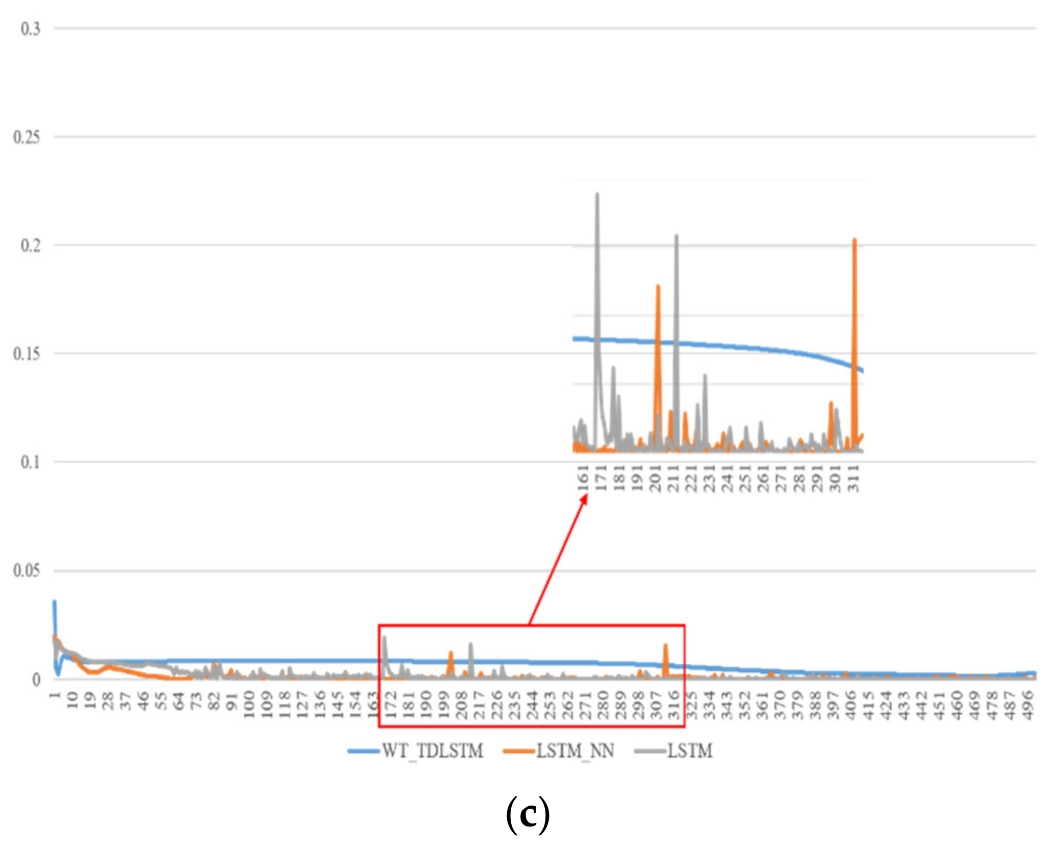
Figure 7a–c show the comparison of convergence curves of different models on the residential, commercial, and industrial monthly electricity price test datasets, respectively. By comparing the convergence process between LSTM, LSTM-NN, and WT_TDLSTM, we can see that the convergence curve of the WT_TDLSTM model has no obvious fluctuations on the three electricity price datasets. More specifically, we find that the greater the number of iterations is, the greater the fluctuation range of the convergence curve of the LSTM and LSTM-NN models in Figure 7a,b. Moreover, the convergence curves of the LSTM and LSTM_NN models fluctuate significantly in Figure 7c. However, as the number of iterations increases, the convergence curve of the WT_TDLSTM model, especially in Figure 7a,b, gradually flattens. The above results illustrate that the denoising ability of the WT_TDLSTM model is better, and the model is more robust.

4. Discussion and Conclusions

In this paper, we propose an electricity price prediction model based on tensor decomposition, a wavelet transform and a long short-term memory. We innovatively propose a tensor decomposition method based on $L_1$ regularization for multiscale data fusion denoising. We have also integrated wavelet transform and LSTM model in the model framework, where wavelet transform is used to remove the noise of the data itself, and the LSTM model is used to achieve high-precision power prediction effects. In the experiment, we fused the data of three time scales and built a 2-layer LSTM model.

The experimental results of these three datasets show that the model proposed in this paper is better than the existing model by 33.65–99.97% in terms of MSE and RMSE. To be more specific, the prediction performance of the WT_TDLSTM model is significantly better than that of the LSTM model, which shows that the use of multiscale data, a wavelet transform, and a tensor for fusion are very helpful to the improvement in the prediction performance of the model. Meanwhile, compared with the baseline models, the WT_TDLSTM model still achieves better prediction performance.

In conclusion, the WT_TDLSTM model can serve as a powerful tool to forecast short-term multiscale electricity prices. If the model can be used in practice, it will play an important role in the operation of the electricity market. Although the model has achieved good results, the WT_TDLSTM model still has some limitations: due to tensor decomposition, the time complexity of the model is relatively high, the tensor operation requires many computing resources, and the memory usage is large. In the future, we plan to further improve the steps of tensor calculation so that it can reduce memory usage and speed up calculations.

References

- Weron, R. Electricity price forecasting: A review of the state-of-the-art with a look into the future. Int. J. Forecast. 2014, 30, 1030–1081. [Google Scholar] [CrossRef] [Green Version]
- Aggarwal, S.K.; Saini, L.M.; Kumar, A. Electricity price forecasting in deregulated markets: A review and evaluation. Int. J. Electr. Power Energy Syst. 2009, 31, 13–22. [Google Scholar] [CrossRef]
- Conejo, A.J.; Plazas, M.A.; Espinola, R.; Molina, A.B. Day-ahead electricity price forecasting using the wavelet transform and ARIMA models. IEEE Trans. Power Syst. 2005, 20, 1035–1042. [Google Scholar] [CrossRef]
- Nowotarski, J.; Weron, R. Recent advances in electricity price forecasting: A review of probabilistic forecasting. Renew. Sustain. Energy Rev. 2018, 81, 1548–1568. [Google Scholar] [CrossRef]
- Li, G.; Liu, C.-C.; Mattson, C.; Lawarrée, J. Day-ahead electricity price forecasting in a grid environment. IEEE Trans. Power Syst. 2007, 22, 266–274. [Google Scholar] [CrossRef]
- Yang, W.; Wang, J.; Niu, T.; Du, P. A novel system for multi-step electricity price forecasting for electricity market management. Appl. Soft Comput. 2020, 88, 106029. [Google Scholar] [CrossRef]
- Kumar, A.; Luthra, S.; Mangla, S.K.; Kazançoğlu, Y. COVID-19 impact on sustainable production and operations management. Sustain. Oper. Comput. 2020, 1, 1–7. [Google Scholar] [CrossRef]
- Li, L.; Chang, L.; Wang, G.; Chen, W.; Ding, Q. Security correction for medium and long-term electricity energy transaction based on security-constrained unit commitment. In Proceedings of the 2018 International Conference on Power System Technology (POWERCON), Guangzhou, China, 6–8 November 2018; pp. 822–827. [Google Scholar]
- Liu, C.; Zhou, M.; Wu, J.; Long, C.; Kundur, D. Financially motivated FDI on SCED in real-time electricity markets: Attacks and mitigation. IEEE Trans. Smart Grid 2017, 10, 1949–1959. [Google Scholar] [CrossRef]
- Yang, Z.; Ce, L.; Lian, L. Electricity price forecasting by a hybrid model, combining wavelet transform, ARMA and kernel-based extreme learning machine methods. Appl. Energy 2017, 190, 291–305. [Google Scholar] [CrossRef]
- Marín, J.B.; Orozco, E.T.; Velilla, E. Forecasting electricity price in colombia: A comparison between neural network, ARMA process and hybrid models. Int. J. Energy Econ. Policy 2018, 8, 97. [Google Scholar]
- Tan, Z.; Zhang, J.; Wang, J.; Xu, J. Day-ahead electricity price forecasting using wavelet transform combined with ARIMA and GARCH models. Appl. Energy 2010, 87, 3606–3610. [Google Scholar] [CrossRef]
- Cui, H.; Song, X. Research on electricity price forecasting based on chaos theory. In Proceedings of the 2008 International Seminar on Future Information Technology and Management Engineering, Leicestershire, UK, 20 November 2008; pp. 398–401. [Google Scholar]
- Singhal, D.; Swarup, K. Electricity price forecasting using artificial neural networks. Int. J. Electr. Power Energy Syst. 2011, 33, 550–555. [Google Scholar] [CrossRef]
- Nogales, F.J.; Conejo, A.J. Electricity price forecasting through transfer function models. J. Oper. Res. Soc. 2006, 57, 350–356. [Google Scholar] [CrossRef]
- Chen, X.; Dong, Z.Y.; Meng, K.; Xu, Y.; Wong, K.P.; Ngan, H. Electricity price forecasting with extreme learning machine and bootstrapping. IEEE Trans. Power Syst. 2012, 27, 2055–2062. [Google Scholar] [CrossRef]
- Zahid, M.; Ahmed, F.; Javaid, N.; Abbasi, R.A.; Zainab Kazmi, H.S.; Javaid, A.; Bilal, M.; Akbar, M.; Ilahi, M. Electricity price and load forecasting using enhanced convolutional neural network and enhanced support vector regression in smart grids. Electronics 2019, 8, 122. [Google Scholar] [CrossRef] [Green Version]
- Mandal, P.; Srivastava, A.K.; Negnevitsky, M.; Park, J.-W. An effort to optimize similar days parameters for ANN based electricity price forecasting. In Proceedings of the 2008 IEEE Industry Applications Society Annual Meeting, Edmonton, AB, Canada, 5–9 October 2008; pp. 1–9. [Google Scholar]
- González, C.; Mira-McWilliams, J.; Juárez, I. Important variable assessment and electricity price forecasting based on regression tree models: Classification and regression trees, Bagging and Random Forests. IET Gener. Transm. Distrib. 2015, 9, 1120–1128. [Google Scholar] [CrossRef]
- Yang, W.; Sun, S.; Hao, Y.; Wang, S. A novel machine learning-based electricity price forecasting model based on optimal model selection strategy. Energy 2022, 238, 121989. [Google Scholar] [CrossRef]
- Khan, S.; Aslam, S.; Mustafa, I.; Aslam, S. Short-Term Electricity Price Forecasting by Employing Ensemble Empirical Mode Decomposition and Extreme Learning Machine. Forecasting 2021, 3, 460–477. [Google Scholar] [CrossRef]
- Wang, D.; Luo, H.; Grunder, O.; Lin, Y.; Guo, H. Multi-step ahead electricity price forecasting using a hybrid model based on two-layer decomposition technique and BP neural network optimized by firefly algorithm. Appl. Energy 2017, 190, 390–407. [Google Scholar] [CrossRef]
- Khan, Z.A.; Fareed, S.; Anwar, M.; Naeem, A.; Gul, H.; Arif, A.; Javaid, N. Short Term Electricity Price Forecasting Through Convolutional Neural Network (CNN). In AINA Workshops: 2020; MDPI: Basel, Switzerland, 2021; pp. 1181–1188. [Google Scholar]
- Badal, L.; Franzén, S. A Comparative Analysis of RNN and SVM: Electricity Price Forecasting in Energy Management Systems; Kth Royal Institute Of Technology: Stockholm, Sweden, 2019. [Google Scholar]
- Huang, C.J.; Shen, Y.; Chen, Y.H.; Chen, H.C. A novel hybrid deep neural network model for short-term electricity price forecasting. Int. J. Energy Res. 2021, 45, 2511–2532. [Google Scholar] [CrossRef]
- Memarzadeh, G.; Keynia, F. Short-term electricity load and price forecasting by a new optimal LSTM-NN based prediction algorithm. Electr. Power Syst. Res. 2021, 192, 106995. [Google Scholar] [CrossRef]
- Guo, X.; Zhao, Q.; Zheng, D.; Ning, Y.; Gao, Y. A short-term load forecasting model of multi-scale CNN-LSTM hybrid neural network considering the real-time electricity price. Energy Rep. 2020, 6, 1046–1053. [Google Scholar] [CrossRef]
- Zadeh, A.; Chen, M.; Poria, S.; Cambria, E.; Morency, L.-P. Tensor fusion network for multimodal sentiment analysis. arXiv 2017, arXiv:170707250 2017. [Google Scholar]
- Zhao, T.; Xu, Y.; Monfort, M.; Choi, W.; Baker, C.; Zhao, Y.; Wang, Y.; Wu, Y.N. Multi-agent tensor fusion for contextual trajectory prediction. In Proceedings of the IEEE/CVF Conference on Computer Vision and Pattern Recognition, Nashville, TN, USA, 20–25 June 2021; pp. 12126–12134. [Google Scholar]
- Wang, T.; Xu, X.; Yang, Y.; Hanjalic, A.; Shen, H.T.; Song, J. Matching images and text with multi-modal tensor fusion and re-ranking. In Proceedings of the 27th ACM International Conference on Multimedia, München, Germany, 20 October 2021; pp. 12–20. [Google Scholar]
- Zhang, D. Wavelet transform. In Fundamentals of Image Data Mining; Springer: Berlin/Heidelberg, Germany, 2019; pp. 35–44. [Google Scholar]
- Arneodo, A.; Grasseau, G.; Holschneider, M. Wavelet transform of multifractals. Phys. Rev. Lett. 1988, 61, 2281. [Google Scholar] [CrossRef]
- Pathak, R.S. The Wavelet Transform, Vol. 4; Springer Science & Business Media: New York, NY, USA, 2009. [Google Scholar]
- Kolda, T.G.; Bader, B.W. Tensor decompositions and applications. SIAM Rev. 2009, 51, 455–500. [Google Scholar] [CrossRef]
- Chachlakis, D.G.; Prater-Bennette, A.; Markopoulos, P.P. L1-norm Tucker tensor decomposition. IEEE Access 2019, 7, 178454–178465. [Google Scholar] [CrossRef]
- Markopoulos, P.P.; Karystinos, G.N.; Pados, D.A. Optimal algorithms for L1-subspace signal processing. IEEE Trans. Signal Process. 2014, 62, 5046–5058. [Google Scholar] [CrossRef] [Green Version]
- Gower, J.C.; Dijksterhuis, G.B. Procrustes Problems, Vol. 30; Oxford University Press on Demand: New York, NY, USA, 2004. [Google Scholar]
- Hochreiter, S.; Schmidhuber, J. Long short-term memory. Neural Comput. 1997, 9, 1735–1780. [Google Scholar] [CrossRef]
- Sundermeyer, M.; Schlüter, R.; Ney, H. LSTM neural networks for language modeling. In Proceedings of the Thirteenth annual Conference of the International Speech Communication Association, Portland, OR, USA, 9–13 September 2012. [Google Scholar]
- Xingjian, S.; Chen, Z.; Wang, H.; Yeung, D.-Y.; Wong, W.-K.; Woo, W.-C. Convolutional LSTM network: A machine learning approach for precipitation nowcasting. In Proceedings of the Advances in Neural Information Processing Systems, Montreal, QC, Canada, 7–12 December 2015; pp. 802–810. [Google Scholar]
- Zhou, C.; Sun, C.; Liu, Z.; Lau, F. A C-LSTM neural network for text classification. arXiv 2015, arXiv:151108630 2015. [Google Scholar]
Figure 1.
Overview of current research methods for EPF problem.
Figure 2.
The process of tensor fusion for electricity price data on multiple scales.
Figure 3.
The training process of LSTM.
Figure 4.
(A) A wavelet transform is used for denoising and tensor fusion in multiscale data fusion. (B) LSTM is used for regression prediction, and matrix M is transformed from the reconstruction tensor.
Figure 5.
Performance of the WT_TDLSTM model with different learning rates on the residential monthly electricity price dataset.
Figure 6.
Fitting effect of different models on test datasets: (a) fitting effect of WT_TDLSTM model on residential monthly electricity price test dataset; (b) fitting effect of LSTM_NN model on commercial monthly electricity price test dataset; (c) fitting effect of LSTM model on industrial monthly electricity price test dataset. The solid line and the dashed line refer to the true value and the predicted value, respectively.
Figure 7.
Comparison of convergence curves of the different models: (a) the change of the convergence curve for LSTM, LSTM-NN, and WT_TDLSTM models on residential monthly electricity price dataset; (b) the change of the convergence curve for LSTM, LSTM-NN, and WT_TDLSTM models on commercial monthly electricity price dataset; (c) the change of the convergence curve for LSTM, LSTM-NN, and WT_TDLSTM models on industrial monthly electricity price dataset.